A Comparative Study of Differential Evolution Variants in Constrained Structural Optimization

1. Introduction

The optimization of structures has been a topic of great interest for both scientists and engineering professionals, especially in recent years. Metaheuristic search algorithms are widely accepted as efficient approaches for handling difficult optimization problems. Such algorithms are designed for solving a wide range of optimization problems in an approximate way, without having to adapt explicitly to every single problem. Moreover, they can be generally applied to problems for which there exists no satisfactory problem-specific algorithm.

In recent years differential evolution (DE) (Storn and Price, 1997) has gained increasing interest for solving optimization problems in many scientific and engineering fields. Today, it is considered one of the most popular optimization algorithms for continuous optimization problems. The method was originally proposed by Storn and Price (1995) for minimizing non-differentiable and possibly nonlinear continuous functions. It is worth noting that although DE is an evolutionary algorithm, it bears no natural paradigm and it is not biologically inspired like most other evolutionary algorithms. DE has exhibited very good performance in a variety of optimization problems from various scientific fields. It belongs to stochastic population-based evolutionary methods and like other evolutionary algorithms, it uses a population of candidate solutions and the search is done in a stochastic way by applying mutation, crossover, and selection operators to drive the population toward better solutions in the design space.

The main advantage of standard DE is the fact that it has only three control parameters that one needs to adjust. The performance of DE in a specific optimization problem depends largely on both the trial vector generation scheme and the choice of the control parameters. First, one needs to choose the trial vector generation scheme and then to adjust the control parameters for the optimization problem in order to achieve good optimization results. Finding the right values of the control parameters is not always easy and can become time consuming and difficult especially for specific hard problems. This has led the researchers to study and develop new advanced DE variants that exhibit adaptive and self-adaptive control parameters. In the case of adaptive parameter control (Eiben et al., 1999), the parameters are adapted based on feedback received during the search process.

Shukla et al. (2017) presented a modified mutation vector generation scheme for the basic DE for solving the stagnation problem. A new variant of DE was proposed and its performance was tested on 24 benchmark functions. Abbas et al. (2015) proposed a tournament-based parent selection variant of the DE algorithm in an effort to enhance the searching capability and improve convergence speed of DE. The paper also describes a statistical comparison of existing DE mutation variants, categorizing these variants based on their overall performance. Charalampakis and Tsiatas (2019) compare variants of Genetic Algorithms, Particle Swarm Optimization (Plevris and Papadrakakis, 2011), Artificial Bee Colony, Differential Evolution, and Simulated Annealing in truss sizing structural optimization problems. The authors claim that for the examined problems, DE is the most reliable algorithm, showing robustness, excellent performance and scalability. Mezura-Montes et al. (2006) present an empirical comparison of several DE variants in solving global optimization problems where 13 benchmark problems from the literature were examined and eight different variants were implemented.

In the present study, we investigate the performance of five popular DE variants in dealing with constrained structural optimization problems. More specific the following five problems are considered:

• The standard differential evolution (DE) (Storn and Price, 1997)

• The composite differential evolution (CODE) (Wang et al., 2011)

• The self-adaptive control parameters differential evolution (JDE) (Brest et al., 2006)

• The adaptive differential evolution with optional external archive (JADE) (Zhang and Sanderson, 2009)

• The self-adaptive differential evolution (SADE) (Qin et al., 2009).

We examine the performance of each algorithm in five structural optimization problems, three plane and two space truss benchmark structures where the objective is to minimize the structural weight subject to constraints on stresses and displacements.

The remainder of the paper is organized as follows. The second section contains the problem definition and the constraint handling scheme. Section 3 describes the standard DE, the most frequently used mutation schemes and the other four DE variants examined in the study. The numerical examples, the relevant results and a discussion on them are presented in section 4. Section 5 discusses the conclusions of the work.

2. Problem Definition

Many problems in structural engineering involve often dealing with a large number of design parameters which can affect the performance of the system. The design and testing of civil engineering structures requires often an iterative process with proper adjustment of the parameters, that can be hard and time consuming. Design optimization offers solutions to this problem by changing the design parameters in an organized and automated manner in an effort to reach an optimal solution. The target of the optimization is usually the minimization of a cost function.

In sizing structural optimization problems, the objective is associated with the minimization of the weight of the structure under some behavioral constraints that have usually to do with displacements and stresses. The design parameters have to do with the dimensions of the cross sections of the structural members. The present study is focused on 2D and 3D truss structures and the design variables are continuous representing the cross-sectional areas of the members of the structure. For such problems the objective function is usually the weight (or mass) of the structure and the problem is formulated as follows:

$\begin{array}{ll}\begin{array}{cc}{\displaystyle \underset{x_i}{min}}& W(\text{x})={\displaystyle \sum _{i=1}^{N_e}}{L}_i{x}_i{\rho }_i\hfill \\ \text{s.t.}& g_k(\text{x})\le 0,k=\left\{1,\dots ,K\right\}\hfill \end{array}& (1)\end{array}$

where W(x) is the total structural weight, N_e is the number of structural elements, x = {x₁, …, x_Ne} is the vector which contains the cross-section areas x_i of all elements, L_i is the length and ρ_i is the material density of element i. In addition, g(x) are the behavioral constraints, K in total. The behavioral constraints are relationships involving usually stresses and deflections of the various elements and nodes of the structure, for example the maximum stress, the maximum deflection, or the minimum load capacity to satisfy norms requirements. Many times, for practical purposes and for uniformity, the areas of particular members are grouped together so that the number of design variables can become significantly smaller than the total number of elements of the structure. This is very convenient especially for big structures with a large number of elements. Grouping in optimization is also in line with actual grouping that is performed in practice due to symmetry and simplicity.

2.1. Constraint Handling

A common practice for dealing with an optimization problem that includes inequality constraints is the use of a penalty function. Such functions can be used to transform the original constrained problem to an unconstrained one. This has been a popular approach for dealing with such problems because it is simple and rather easy to implement. In the present study, the following penalty formulation is used to handle the optimization problem constraints:

$\begin{array}{ll}F(\text{x})=f(\text{x})+P(\text{x})=f(\text{x})+\mu {\displaystyle \sum _{k=1}^N}{H}_k(\text{x})g_k^2(\text{x})& (2)\end{array}$

where f(x) is the objective function to be minimized, P(x) is the penalty term, g_k(x) is the k-th constraint function in the form g_k(x) ≤ 0, μ ≥ 0 is a penalty factor that should be large enough (e.g., 10⁶) and the H_k(x) function is defined as follows:

$\begin{array}{ll}{H}_i(\text{x})=\{\begin{array}{cc}1,& \text{if }{g}_i(\text{x})>0\hfill \\ 0,& \text{otherwise}\hfill \end{array}& (3)\end{array}$

3. Optimization Algorithms

3.1. Standard DE

DE is a popular optimization method used for multidimensional real-valued functions which uses a population of individual solutions. The method does not require gradient information, which means that the optimization problem does not need to be differentiable. The algorithm searches the design space by maintaining a population of candidate solutions (individuals) and creating new solutions by combining existing ones according to a specific process. The candidates with the best objective values are kept in the next iteration of the algorithm in a manner that the new objective value of an individual is improved forming consequently part of the population, otherwise the new objective value is discarded. The process repeats itself until a given termination criterion is satisfied.

Let x ∈ ℝ^D designate a candidate solution in the current population, where D is the dimensionality of the problem being optimized and f : ℝ^D → ℝ is the objective function to be minimized. The basic DE algorithm, following the “DE/rand/1” scheme, can be described schematically as follows:

ALGORITHM 1

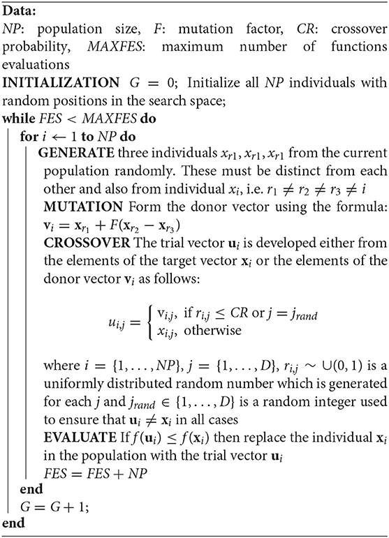
Algorithm 1. Pseudocode of DE.

In every generation (iteration) G, Differential Evolution uses the mutation operator for producing the donor vector v_i for each individual x_i in the current population. For each target vector x_i = {x_{i, 1}, …, x_{i, D}} at generation G, the associated mutant vector v_i = {v_{i, 1}, …, v_{i, D}} can be produced using a specific mutation scheme. The six most widely used mutation schemes in differential evolution are described below:

$\begin{array}{rr}\text{“DE/rand/1”}& \hfill {\text{v}}_i={\text{x}}_{r_1}+F({\text{x}}_{r_2}-{\text{x}}_{r_3})\hfill \\ \text{“DE/best/1"}& \hfill {\text{v}}_i={\text{x}}_{best}+F({\text{x}}_{r_1}-{\text{x}}_{r_2})\hfill \\ \text{“DE/rand/2”}& \hfill {\text{v}}_i={\text{x}}_{r_1}+F({\text{x}}_{r_2}-{\text{x}}_{r_3})+F({\text{x}}_{r_4}-{\text{x}}_{r_5})\hfill \\ \text{“DE/best/2”}& \hfill {\text{v}}_i={\text{x}}_{best}+F({\text{x}}_{r_1}-{\text{x}}_{r_2})+F({\text{x}}_{r_3}-{\text{x}}_{r_4})\hfill \\ \text{“DE/current-to-best/1”}& \hfill {\text{v}}_i={\text{x}}_i+F({\text{x}}_{best}-{\text{x}}_i)+F({\text{x}}_{r_1}-{\text{x}}_{r_2})\hfill \\ \text{“DE/current-to-rand/1”}& \hfill {\text{v}}_i={\text{x}}_i+rand({\text{x}}_{r_1}-{\text{x}}_i)+F({\text{x}}_{r_2}-{\text{x}}_{r_3})\hfill \end{array}$

where the indices r₁, r₂, r₃, r₄, r₅ are random integers which are mutually exclusive, within the range [1, NP] and are also different than index i (r₁ ≠ r₂ ≠ r₃ ≠ r₄ ≠ r₅ ≠ i). These indices are generated once for each mutant vector. F is the scaling factor, a positive control parameter for scaling the difference vector, while x_best is the best individual vector, i.e., the individual with the best objective value in the population at the current generation G.

The main advantage of DE is the fact that it has only three control parameters that the user of the algorithm needs to adjust. These include the population size NP, where NP ≥ 4, the mutation factor (or differential weight, or scaling factor) F ∈ [0, 2] and the crossover probability (or crossover control parameter) CR ∈ [0, 1]. In the standard DE these control parameters were kept fixed for all the optimization process. The population size has a significant influence on the ability of the algorithm to explore. In case of problems with a large number of dimensions, the population size needs also to be large to make the algorithm capable of searching in the multi-dimensional design space. A population size of 30–50 is usually sufficient in most problems of engineering interest. The mutation factor F is a positive control parameter for scaling and controlling the amplification of the difference vector. Small values of F will lead to smaller mutation step sizes and as a result it will take longer for the algorithm to converge. Large values of F facilitate exploration, but can lead to the algorithm overshooting good optima. Thus, the value has to be small enough to enhance local exploration but also large enough to maintain diversity. The crossover probability CR has an influence on the diversity of DE, as it controls the number of elements that will change. Larger values of CR will lead to introducing more variation in the new population, therefore increasing it increases exploration. But again a compromise value has to be found to ensure both local and global search capabilities.

3.2. CODE

Studies have shown that both the control parameters and the schemes for the trial vector generation can have a significant influence on the algorithm's performance. Different trial vector generation schemes and control parameters can be therefore combined to improve the performance of the optimization process for different kinds of problems. Mallipeddi et al. (2011) was the first to attempt, trying to combine various schemes for trial vector generation with different control parameter settings.

ALGORITHM 2

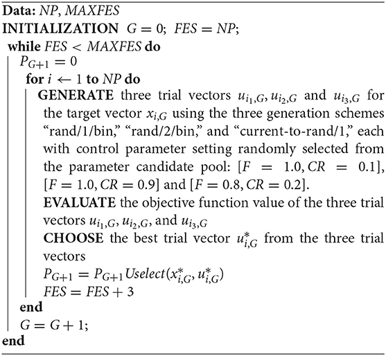
Algorithm 2. Pseudocode of CODE.

Composite DE (CODE) (Wang et al., 2011) is based on the idea of randomly combining a number of trial vector generation schemes with several control parameter settings at each generation, for the creation of new trial vectors. These combination schemes are based on experimental results from the literature. In particular, CODE uses three different trial vector generation schemes and three control parameter settings, combining them randomly for the generation of trial vectors. The structure of CODE is rather simple, and the algorithm is easy to implement. The three trial vector generation schemes of the method are the following: (i) “rand/1/bin”; (ii) “rand/2/bin”; (iii) “current-to-rand/1.” It has to be noted that in the case of the “current-to-rand/1”scheme, the binominal crossover operator is not applied. The three control parameter settings used are the following: (1) F = 1.0 and CR = 0.1; (2) F = 1.0 and CR = 0.9; (3) F = 0.8 and CR = 0.2.

In each generation, three trial vectors are generated for each target vector as follows: each of the three trial vector generation schemes is combined with a control parameter setting from the relevant pool, in a random manner. If the best one of the three is better than its target vector, then it enters the next generation. The pseudocode of the method is presented in Algorithm 2.

3.3. JDE

The standard DE algorithm includes a set of parameters that are kept fixed throughout the optimization process. These parameters would need to be adjusted for every single optimization problem in order to ensure optimal performance. Some researchers have claimed that the DE parameters are not so difficult to set manually (Storn and Price, 1997). Yet, others (Gamperle et al., 2002) claim that the process can be quite demanding especially for particular optimization problems. According to Liu and Lampinen (2002), the effectiveness, efficiency, and robustness of the DE algorithm are very sensitive to the values of the control parameters, while certain parameters may work well in a problem but not so well with other problems, which makes the optimal selection of the parameters a problem-specific question.

JDE features self-adaptive control parameter settings and has shown acceptable performance on benchmark problems (Brest et al., 2006). It uses the idea of the evolution of the evolution, i.e., it uses an evolution process to fine tune the optimization algorithm parameters. Although the idea sounds promising, the proof of convergence of self-adaptation algorithms is a difficult task in general. In JDE the parameter control technique is based on the self-adaptation of the parameters F and CR of the DE evolutionary process, producing a flexible DE which adjusts itself in order to achieve the best optimization outcome. According to Storn and Price (1997), DE behavior is more sensitive to the choice of F than it is to the choice of CR. The study suggests the values of [0.5, 1] for F, [0.8, 1] for CR and 10D for NP, where D is the number of dimensions of the problem. The control parameters of the JDE algorithm are described as:

$\begin{array}{ll}{F}_{i,G+1}=\{\begin{array}{ll}{F}_l+ran{d}_1{F}_u,& \text{if }ran{d}_2<{\tau }_1\\ F_{i,G},& \text{otherwise}\end{array}& (4)\end{array}$

$\begin{array}{ll}C{R}_{i,G+1}=\{\begin{array}{ll}ran{d}_3,& \text{if }ran{d}_4<{\tau }_2\\ C{R}_{i,G},& \text{otherwise}\end{array}& (5)\end{array}$

where rand_j with j ∈ {1, 2, 3, 4} are uniform random values in [0, 1] and τ₁, τ₂ represent probabilities to adjust factors F and CR with suggested values τ₁ = τ₂ = 0.10, while F_l = 0.1 and F_u = 0.9 and as a result the new F takes values in the range [0.1, 1]. The new CR takes values in [0, 1]. The new control parameter values take effect before the mutation and as a result they influence the mutation, crossover and selection operations of the new trial vector. The idea of JDE is that one does not need to guess good values of F and CR any more. The rules for self-adaptation of the two parameters are quite simple and easy to implement and use and as a result JDE does not increase significantly the complexity or the computational effort of the standard DE method. Experimental results have shown that JDE outperforms both the classic “DE/rand/1” and other schemes (Liu and Lampinen, 2005). The main contribution of JDE is that the user no longer needs to guess good values of F and CR, which are problem-dependent.

3.4. JADE

The selection of the values of the mutation factor (F) and the crossover probability (CR) can significantly affect the performance of DE. Trial-and-error attempts for fine-tuning these control parameters can be successful but they require much time and effort and the result is always problem-specific. Researchers have suggested various self-adaptive mechanisms for dealing with this problem (Qin and Suganthan, 2005; Brest et al., 2006, 2007; Huang et al., 2006; Teo, 2006) in an effort to dynamically update the control parameters without having any prior knowledge of the characteristics of the problem.

JADE was proposed to improve the performance of the standard DE by implementing a new mutation scheme which updates control parameters in an adaptive way. The method introduces a new mutation scheme denoted as “DE/current-to-pbest” with an optional external archive. The algorithm, as described in Zhang and Sanderson (2009) utilizes not only the best solution, but a number of 100p%, p ∈ (0, 1] good solutions. Compared to “DE/rand/k,” greedy schemes such as the “DE/current-to-best/k” and the “DE/best/k” can benefit from their fast convergence by incorporating best solution information in the search procedure. However, this best solution information can also cause premature convergence problems due to reduced diversity in the population.

In the “DE/current-to-pbest/1” scheme (without archive), a mutation vector is generated as follows:

$\begin{array}{ll}{\text{v}}_{i,g}={\text{x}}_{i,g}+F_i({\text{x}}_{best,g}^p-{\text{x}}_{i,g})+F_i({\text{x}}_{r1,g}-{\text{x}}_{r2,g})& (6)\end{array}$

Where ${\text{x}}_{best}^p$ is chosen randomly as one of the top 100p% individuals of the current population with p ∈ (0, 1], and F_i is the mutation factor associated with x_i. In JADE, any of the top 100p% solutions can be randomly chosen to play the role of the single best solution in the standard “DE/current-to-best” scheme. This is because recently explored solutions that are not the best can still provide additional information about the desired search direction. In the “DE/current-to-pbest/1” scheme with archive, a mutation vector is generated as follows:

$\begin{array}{ll}{\text{v}}_{i,g}={\text{x}}_{i,g}+F_i({\text{x}}_{best,g}^p-{\text{x}}_{i,g})+F_i({\text{x}}_{r1,g}-{\tilde{x}}_{r2,g})& (7)\end{array}$

Where x_{i, g}, x_{r1, g} and $x_{best,g}^p$ are selected from the current population P in the usual way, while ${\tilde{x}}_{r2,g}$ is randomly chosen individual (distinct from x_{i, g} and x_{r1, g}) from the union P∪A of the current population and the set of archived inferior solutions A. The archive is initiated as empty. Consequently, after each iteration, the parent solutions that fail in the selection process are added to the archive. If the size of the archive exceeds a predefined value, for example NP, then some solutions are removed from the archive randomly. The “DE/current-to-pbest/1” scheme (without archive) is a special case of the “DE/current-to-pbest/1” scheme with archive, if we set the archive size equal to zero (i.e., empty archive). Numerical results have shown that JADE exhibits superior or at least comparable performance to other standard or adaptive DE algorithms (Zhang and Sanderson, 2009).

3.5. SADE

In SADE, both the trial vector generation schemes and their associated control parameter values can be gradually self-adapted according to their previous experiences of generating promising solutions (Qin et al., 2009). The method consists a self-adaptive DE variant, in which one trial vector generation scheme is selected from the candidate pool according to the probability learned from its success rate in generating improved solutions within a certain number of previous generations LP (learning period). The selected scheme is then applied to the corresponding target vector in order to obtain the trial vector. At each generation, the sum of the probabilities of choosing a scheme from the candidate pool are equal to 1.

In the beginning, all schemes have an equal probability to be selected, i.e., the probabilities with respect to each scheme are initialized as 1/K, where K is the total number of schemes. The population size NP remains a user-specified parameter because it has to do with the complexity of the given optimization problem. The parameter F is approximated by a normal distribution with mean value 0.5 and a standard deviation of 0.3 which makes F fall within the range [−0.4, 1.4] with a probability of 0.997. The control parameter K in the “DE/current-to-rand/1” scheme is randomly generated within [0,1] while CR is assumed to follow a normal distribution with mean value CR_m and standard deviation Std, where initially it is set CR_m = 0.5 and Std = 0.1. A set of random CR values is generated following the normal distribution and then applied to those target vectors to which the k-th scheme is assigned.

To adapt the CR values, memories CRMemory_k are established to store those CR values with respect to the k-th scheme of successfully trial vectors generation, entering the next generation within the previous LP generations that keep the success and failure memories by storing CR values. During the first LP generations, CR values with respect to the k-th scheme are drawn from the normal distribution. At each generation after LP generations, the median value that stored in CRMemory_k will be calculated to overwrite CR_mk. After evaluating the newly generated trial vectors, CR values in CRMemory_k that correspond to earlier generations will be replaced by promising CR values obtained at the current generation with respect to the k-th scheme. The method is described in detail in Qin et al. (2009).

4. Numerical Examples

The performance of each of the five optimization algorithms (the standard DE and the four DE variants) is examined in five well-known benchmark structural engineering test examples. The characteristics of each test example is given in Table 1. All test examples have been previously optimized by many researchers (Lee and Geem, 2004; Farshi and Alinia-ziazi, 2010; Gandomi et al., 2013; Talatahari et al., 2013) using various optimization algorithms.

TABLE 1

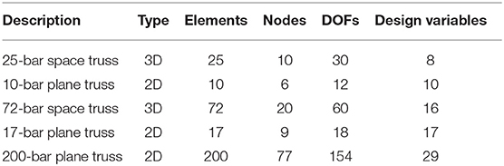
Table 1. Characteristics of the five test problems.

For all test examples the objective is the minimization of the structural weight under constraints on stresses and displacements. The parameters of the optimization algorithms are the following: population size NP = 30, mutation factor F = 0.6, crossover probability CR = 0.9. More specifically, for the JDE variant, τ₁, and τ₂ probabilities are both taken equal to 0.1. JADE is used with the optional archive, with archive size equal to NP = 30, while p = 0.05. The maximum number of objective function evaluations is used as the termination criterion for all cases, with a value of 10⁵. The value of μ used in Equation (2) is equal to 10¹⁰. Furthermore, 30 independent runs have been conducted for each method examined and the convergence history results presented are the average results of the different runs. Other statistical quantities and measures are also presented, such as best, worst, mean, median, standard deviation, and coefficient of variation (COV).

4.1. 25-Bar Space Truss

The first test example is a 25-member space truss. The geometry of the structure is shown in Figure 1A where the dimensions a, b and h are equal to 200, 75, and 100 in, respectively. The density of the material is ρ = 0.1 lb/in³ and the Young's modulus is E = 10,000 ksi. There are two load cases, as shown in Table 2. There are eight groups where the members of the structure belong to. The cross section areas of each design group, in the range [0.01, 5] (in²), are the design variables of the problem. The design variable groups and the stress constraints for each group are shown in Table 3. The maximum allowable displacement for each node is d_max = ±0.35 in every direction. The convergence history of the various DE methods is shown in Figure 1B as the average of 30 independent runs for each optimization algorithm.

FIGURE 1

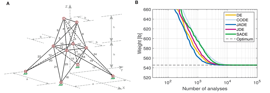
Figure 1. 25-bar space truss (A) geometry; (B) algorithms' convergence histories (average of 30 runs).

TABLE 2

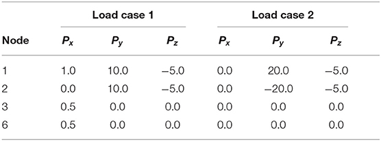
Table 2. 25-bar space truss: Load cases (loads in kips).

TABLE 3

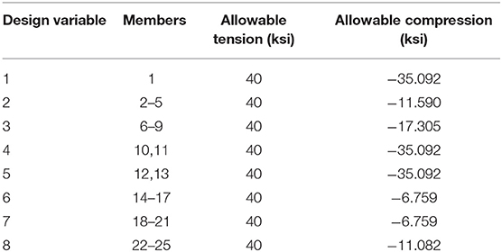
Table 3. 25-bar space truss: allowable stresses for each design group.

Figure 1B shows the convergence history of the five algorithms. The horizontal dashed line represents the best solution ever found in the literature for this specific problem, for comparison purposes. The convergence histories reveal that all the five algorithms eventually manage to converge to approximately the same final result. However, the rate of convergence is different. JADE is the fastest, converging to the optimum earlier than the other algorithms. JADE, DE, and JDE appear to be ranked 1st, 2nd, and 3rd as far as the convergence speed is concerned. Then come SADE and CODE with similar convergence performance. Table 4 reveals that all algorithms managed to find the same best solution (545.555). It is worth noting that three of them managed to find the same best solution in all 30 runs, as the best value and the worst value are the very same. Only JDE and SADE failed to deliver the best solution in all 30 runs, but again the difference is very small and the coefficient of variation has very small values equal to 1.92E-5 and 2.24E-4 for the two methods, respectively.

TABLE 4

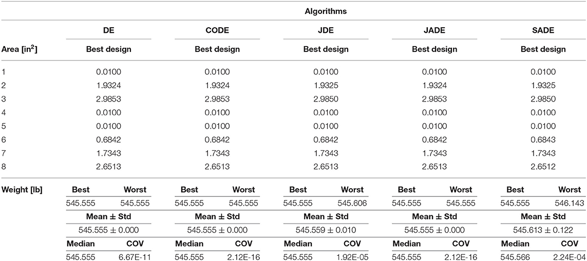
Table 4. Algorithms' statistical parameters for the 25-bar space truss problem.

4.2. 10-Bar Plane Truss

The second test example is the standard benchmark 10-bar plane truss problem. The geometry of the structure is shown in Figure 2A. The characteristics of the structure are: Young's modulus E = 10,000 ksi, density of the material ρ = 0.1 lb/in³, L = 360 in, P = 100 kip. There are 10 group members, i.e., each member of the structure belongs to its own group. The design variables represent the cross-section areas of each structural element in the interval [0.1, 35] (in²). The maximum allowable stress (absolute value) is σ_allow = 25 ksi in tension or compression while the maximum allowable displacement in the ±x and ±y directions for each node is d_max = 2 in. The convergence history of the various DE methods is shown in Figure 2B as the average of 30 independent runs for each optimization algorithm.

FIGURE 2

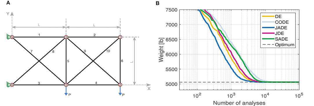
Figure 2. 10-bar plane truss (A) geometry; (B) algorithms' convergence histories (average of 30 runs).

Figure 2B shows that all methods converge to the optimum, but with different convergence rates. Again JADE shows the best convergence performance. The algorithms are ranked as JADE–DE–JDE–SADE–CODE from the fastest to the slowest in reaching the optimum. Table 5 shows that all algorithms managed to find the optimum solution as their “best” run. DE and CODE were very successful in achieving the optimum result even in their “worst” runs. DE and CODE show very consistent performance in all runs and JADE is also good in that. JDE and SADE have the most variation in their results with values of COV equal to 5.68E-4 and 1.21E-3, respectively. It is worth noting that CODE exhibits the slowest convergence but simultaneously the most consistent behavior in reaching the same optimum value in all runs.

TABLE 5

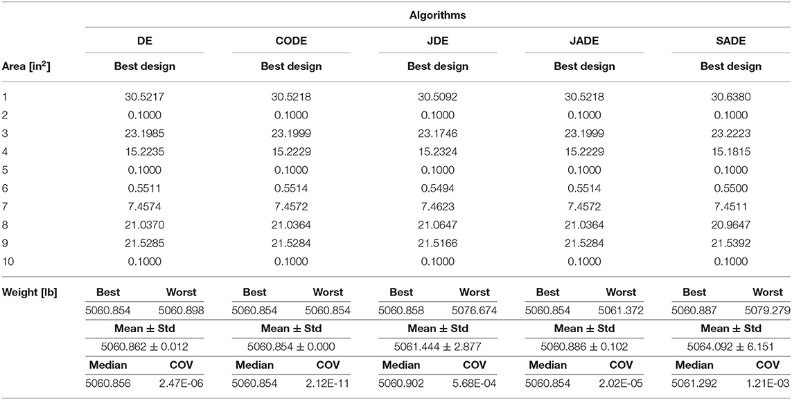
Table 5. Algorithms' statistical parameters for the 10-bar plane truss problem.

4.3. 72-Bar Space Truss

Figure 3A shows the third test example, a space truss with 72 members. The basis of the structure is a rectangle with 2b = 120 in, while the total height is 4b = 240 in. Nodes 1, 2, 3, and 4 are pinned on the ground while all the other nodes are free to move in all three directions. Each member has the following material characteristics: Young's modulus is E = 10,000 ksi and material density ρ = 0.1 lb/in³. Two load cases have been considered. There are 16 groups of structural members. The design variables represent the cross-section areas of each group. There is no upper limit, while the lower limit is 0.01 in² for each design variable. The constraints are imposed on displacements and stresses. The maximum allowable stress (as an absolute value) is σ_allow = 25 ksi, in tension or compression, while the maximum allowable displacement in the ±x and ±y directions is d_max = 0.25 in, for each node. The convergence history of the various DE variants is shown in Figure 3B as the average of 30 independent runs for each method.

FIGURE 3

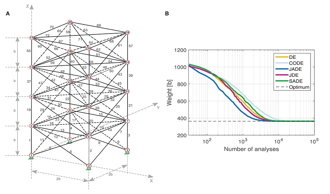
Figure 3. 72-bar space truss (A) geometry; (B) algorithms' convergence histories (average of 30 runs).

Again, Figure 3B shows that all methods converge to the same result with JADE being the fastest. The ranking from fastest to slowest convergence is now JADE–JDE–DE–SADE–CODE. Once again, CODE is very successful in obtaining almost the same optimum value in all runs (COV = 6.89E-6) as shown in Table 6. SADE exhibits the worst performance in terms of variation of the results (COV = 1.04E-3). In any case, all algorithms are again quite successful in almost all their 30 runs.

TABLE 6

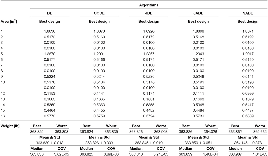
Table 6. Algorithms' statistical parameters for the 72-bar space truss problem.

4.4. 17-Bar Plane Truss

The fourth test example is a 17-bar plane truss. The geometry of the structure is shown in Figure 4A where dimension L is equal to 100 in. The density of the material is ρ = 0.268 lb/in³ and the Young's modulus is E = 30,000 ksi. The structure is subjected to the concentrated load P at node 9 equal to 100 kip. There is no grouping of members in this example, i.e., each member belongs to its own group and there are 17 groups in total. The design parameters, in the interval [0.1, 35] (in²), are the cross-section areas of each member group. The maximum allowable stress (absolute value) is σ_allow = 50 ksi in tension or compression, while the maximum allowable displacement in the ±x and ±y directions is d_max=2 in, for each node. The convergence history of the various DE methods is shown in Figure 4B as the average of 30 independent runs for each optimization algorithm.

FIGURE 4

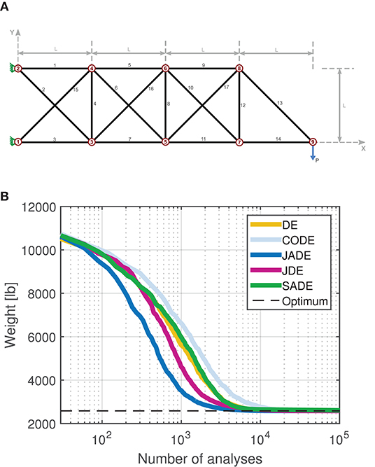
Figure 4. 17-bar plane truss (A) geometry; (B) algorithms' convergence histories (average of 30 runs).

JADE is the fastest algorithm to converge, as shown in Figure 4B, while all algorithms reach the same solution eventually. Table 7 shows that CODE exhibits the most stable performance with COV = 8.12E-7 as far as the final optimum is concerned. SADE has the most variation of the results with COV = 8.15E-3.

TABLE 7

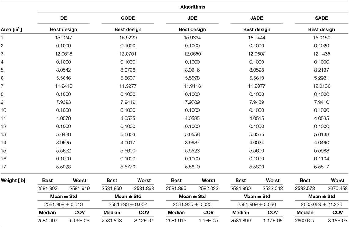
Table 7. Algorithms' statistical parameters for the 17-bar plane truss problem.

4.5. 200-Bar Plane Truss

The fifth example is a space truss consisting of 200 members. The geometry of the structure is shown in Figure 5A where dimensions a, b, and c are equal to 360, 144, and 240 in, respectively. The density of the material is ρ = 0.283 lb/in³ and the Young's modulus is E = 30,000 ksi. There are three independent load cases (LC) as shown in Figure 5A: (i) LC1: 1.0 kip acting in the positive x-direction (blue arrows); (ii) LC2: 10 kips acting in the negative y-direction (orange arrows) and (iii) LC3: the first two load cases acting together.

FIGURE 5

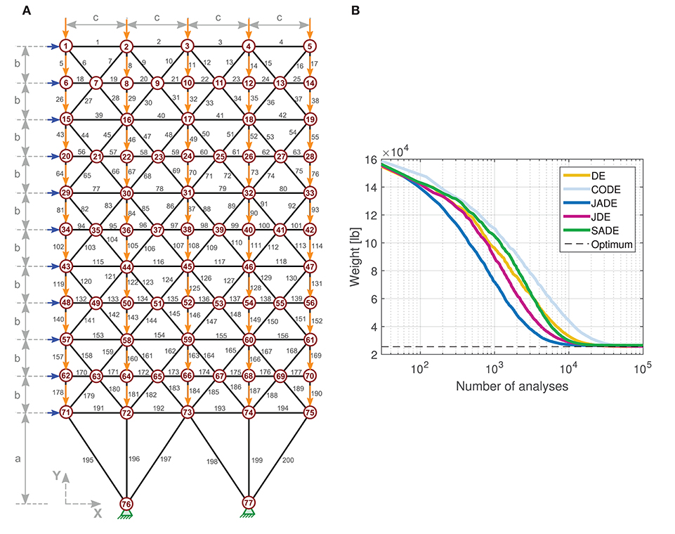
Figure 5. 200-bar plane truss (A) geometry. Load Cases 1 and 2 are depicted with blue and orange arrows, respectively; (B) algorithms' convergence histories (average of 30 runs).

The members of the structure are divided into 29 groups in total, as shown in Table 8. The cross-section areas of each member group, in the interval [0.1, 35] (in²), are the design variables of the problem. The stress of each member, in absolute terms, needs to be less than σ_allow = 10 ksi (in tension or compression). No displacement limit is set for this problem.

TABLE 8

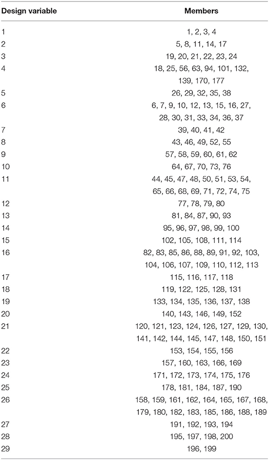
Table 8. 200-bar space truss: Design variable groups.

The convergence history of the various DE methods is shown in Figure 5B as the average of 30 independent runs for each optimization algorithm.

In this problem, JADE is again the fastest algorithm to converge to the final result, followed by JDE. Table 9 shows that CODE exhibits the most stable performance with COV = 4.68E-3 as far as the final optimum is concerned. SADE has the most variation of the results (worst performance) with COV = 1.95E-2. The difference between the best and the worst solutions are 396.171 in CADE and 1901.913 in SADE.

TABLE 9

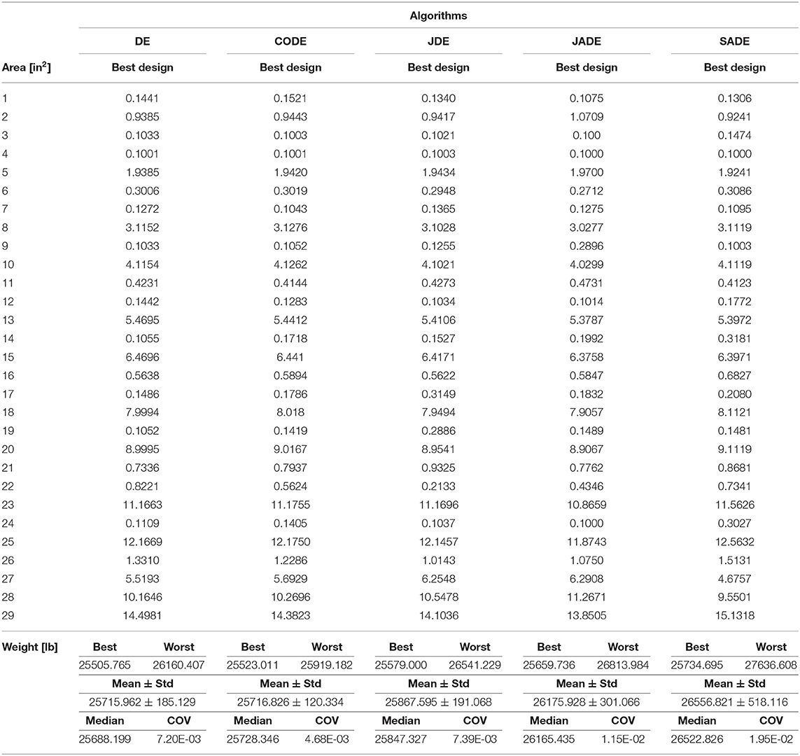
Table 9. Algorithms' statistical parameters for the 200-bar plane truss problem.

5. Discussion

The convergence history plots show that in all problems, JADE converges faster to the final result, followed by JDE and DE which exhibit similar performance with each other in terms of convergence speed. It appears that in the JADE algorithm, the parameter adaptation is beneficial in accelerating the convergence performance of DE by automatically updating the control parameters during the optimization search. This has effect even in the very first iterations of the algorithm, making JADE clearly stand out from the other variants, from the beginning of the search process. CODE exhibits the slowest convergence performance among the five algorithms. All algorithms manage to reach the final result with efficient accuracy in most of the optimization runs. CODE shows the most robust performance among all algorithms as it manages to find the same solution in almost all the optimization runs, with very small variation of the results among the 30 runs. CODE has the lowest values of the coefficient of variation (COV) metric in all five test problems, as shown in Figure 6 (y-values in logarithmic scale). SADE shows the most variation of the results (highest values of COV). CODE guarantees very robust final results but at the expense of slower convergence speed, while JADE manages to provide satisfactory convergence speed and a good quality of the final optimum result. The performance of the standard DE algorithm is also rather good as DE manages to outperform some of the other adaptive schemes.

FIGURE 6

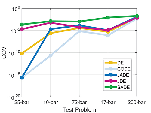
Figure 6. Coefficient of variation (COV) values for each problem and algorithm.

6. Conclusions

The present study investigates the performance of five DE variants, DE, CODE, JDE, JADE, and SADE, in dealing with constrained structural optimization problems. The structures examined are 2D and 3D trusses under single or multiple loading conditions. The constraints are imposed on stresses and displacements while the objective is to minimize the weight of each structure. Five well-known benchmark problems of truss structures have been considered in the comparison. In order to ensure neutrality and to compare the results of the various algorithms, 30 runs have been conducted for each test problem and each algorithm and various statistical metrics have been calculated.

From the statistical analysis that has been conducted, it can be concluded that the CODE algorithm guarantees robustness but with slower convergence speed, while JADE manages to provide a satisfactory compromise between the convergence speed and the quality of the final optimum result, compared to the other four competitors. Surprisingly, even in the case of the standard DE algorithm the performance is rather good as DE manages to outperform some other adaptive schemes, such as SADE, in terms of the quality of the final result and the convergence speed achieved. The same finding has also been reported by Charalampakis and Tsiatas (2019).

Data Availability Statement

The raw data supporting the conclusions of this article will be made available by the authors, without undue reservation.

Author Contributions

MG did the data collection, contributed in the numerical analysis of the test examples, analyzed and interpreted the data, and wrote parts of the paper. VP contributed in the conception and design of the work, analyzed and interpreted the data, wrote parts of the paper, and supervised the overall research work. All authors have made a substantial, direct and intellectual contribution to the work, and approved it for publication.

Conflict of Interest

The authors declare that the research was conducted in the absence of any commercial or financial relationships that could be construed as a potential conflict of interest.

References

Abbas, Q., Ahmad, J., and Jabeen, H. (2015). A novel tournament selection based differential evolution variant for continuous optimization problems. Math. Probl. Eng. 2015:205709. doi: 10.1155/2015/205709

CrossRef Full Text | Google Scholar

Brest, J., Bokovic, B., Greiner, S., Aumer, V., and Maucec, M. S. (2007). Performance comparison of self-adaptive and adaptive differential evolution algorithms. Soft Comput. 11, 617–629. doi: 10.1007/s00500-006-0124-0

CrossRef Full Text | Google Scholar

Brest, J., Greiner, S., Boskovic, B., Mernik, M., and Zumer, V. (2006). Self-adapting control parameters in differential evolution: a comparative study on numerical benchmark problems. IEEE Trans. Evol. Comput. 10, 646–657. doi: 10.1109/TEVC.2006.872133

CrossRef Full Text | Google Scholar

Charalampakis, A. E., and Tsiatas, G. C. (2019). Critical evaluation of metaheuristic algorithms for weight minimization of truss structures. Front. Built Environ. 5:113. doi: 10.3389/fbuil.2019.00113

CrossRef Full Text | Google Scholar

Eiben, A., Hinterding, R., and Michalewicz, Z. (1999). Parameter control in evolutionary algorithms. IEEE Trans. Evol. Comput. 3, 124–141. doi: 10.1109/4235.771166

CrossRef Full Text | Google Scholar

Farshi, B., and Alinia-ziazi, A. (2010). Sizing optimization of truss structures by method of centers and force formulation. Int. J. Solids Struct. 47, 2508–2524. doi: 10.1016/j.ijsolstr.2010.05.009

CrossRef Full Text | Google Scholar

Gamperle, R., Mller, S. D., and Koumoutsakos, P. (2002). A Parameter Study for Differential Evolution. Technical Report WSEAS NNA-FSFS-EC 2002, Interlaken.

Google Scholar

Gandomi, A. H., Talatahari, S., Yang, X.-S., and Deb, S. (2013). Design optimization of truss structures using cuckoo search algorithm. Struct. Design Tall Spec. Build. 22, 1330–1349. doi: 10.1002/tal.1033

CrossRef Full Text | Google Scholar

Huang, V. L., Qin, A. K., and Suganthan, P.N. (2006). “Self-adaptive differential evolution algorithm for constrained real- parameter optimization,” in 2006 IEEE International Conference on Evolutionary Computation (Vancouver, BC), 17–24. doi: 10.1109/CEC.2006.1688285

CrossRef Full Text | Google Scholar

Lee, K. S., and Geem, Z. W. (2004). A new structural optimization method based on the harmony search algorithm. Comput. Struct. 82, 781–798. doi: 10.1016/j.compstruc.2004.01.002

CrossRef Full Text | Google Scholar

Liu, J., and Lampinen, J. (2002). “On setting the control parameter of the differential evolution method,” in Proceedings of MENDEL 2002, 8th International Conference Soft Computing (Brno), 11–18.

PubMed Abstract | Google Scholar

Liu, J., and Lampinen, J. (2005). A fuzzy adaptive differential evolution algorithm. Soft Comput. 6, 448–462. doi: 10.1007/s00500-004-0363-x

CrossRef Full Text | Google Scholar

Mallipeddi, R., Suganthan, P. N., Pan, Q. K., and Tasgetiren, M. F. (2011). Differential evolution algorithm with ensemble of parameters and mutation strategies. Appl. Soft Comput. 11, 1679–1696. doi: 10.1016/j.asoc.2010.04.024

CrossRef Full Text | Google Scholar

Mezura-Montes, E., Velzquez-Reyes, J., and Coello, C. A. C. (2006). “A comparative study of differential evolution variants for global optimization,” in GECCO '06: Proceedings of the 8th Annual Conference on Genetic and Evolutionary Computation (Seattle, WA), 485–492. doi: 10.1145/1143997.1144086

CrossRef Full Text | Google Scholar

Plevris V. and Papadrakakis, M. (2011). A hybrid particle swarm–gradient algorithm for global structural optimization. Comput. Aided Civil Infrastruct. Eng. 26, 48–68. doi: 10.1111/j.1467-8667.2010.00664.x

CrossRef Full Text | Google Scholar

Qin, A. K., Huang, V. L., and Suganthan, P. N. (2009). Differential evolution algorithm with strategy adaptation for global numerical optimization. IEEE Trans. Evol. Comput. 13, 398–417. doi: 10.1109/TEVC.2008.927706

CrossRef Full Text | Google Scholar

Qin, A. K., and Suganthan, P. N. (2005). “Self-adaptive differential evolution algorithm for numerical optimization,” in 2005 IEEE Congress on Evolutionary Computation (Edinburgh), 1785–1791. doi: 10.1109/CEC.2005.1554904

CrossRef Full Text | Google Scholar

Shukla, R., Hazela, B., Shukla, S., Prakash, R., and Mishra, K. K. (2017). “Variant of differential evolution algorithm,” in Advances in Computer and Computational Sciences. Advances in Intelligent Systems and Computing, Vol. 553, eds S. Bhatia, K. Mishra, S. Tiwari, and V. Singh (Singapore: Springer), 601–608. doi: 10.1007/978-981-10-3770-2_56

CrossRef Full Text | Google Scholar

Storn, R., and Price, K. (1995). Differential Evolution—A Simple and Efficient Adaptive Scheme for Global Optimization Over Continuous Spaces. Technical Report, Berkeley, CA. Available online at: https://www.icsi.berkeley.edu/ftp/global/global/pub/techreports/1995/tr-95-012.pdf

Google Scholar

Storn, R., and Price, K. (1997). Differential evolution–a simple and efficient heuristic for global optimization over continuous spaces. J. Glob. Optim. 11, 341–359. doi: 10.1023/A:1008202821328

CrossRef Full Text | Google Scholar

Talatahari, S., Kheirollahi, M., Farahmandpour, C., and Gandomi, A. H. (2013). A multi-stage particle swarm for optimum design of truss structures. Neural Comput. Appl. 23, 1297–1309. doi: 10.1007/s00521-012-1072-5

CrossRef Full Text | Google Scholar

Teo, J. (2006). Exploring dynamic self-adaptive populations in differential evolution. Soft Comput. 10, 673–686. doi: 10.1007/s00500-005-0537-1

CrossRef Full Text | Google Scholar

Wang, Y., Cai, Z., and Zhang, Q. (2011). Differential evolution with composite trial vector generation strategies and control parameters. IEEE Trans. Evol. Comput. 15, 55–66. doi: 10.1109/TEVC.2010.2087271

CrossRef Full Text | Google Scholar

Zhang, J., and Sanderson, A. C. (2009). Jade: Adaptive differential evolution with optional external archive. IEEE Trans. Evol. Comput. 13, 945–958. doi: 10.1109/TEVC.2009.2014613

PubMed Abstract | CrossRef Full Text | Google Scholar