Conceptual Study of a Real-Time Hybrid Simulation Framework for Monopile Offshore Wind Turbines Under Wind and Wave Loads

Introduction

As an emerging field of wind power generation, offshore wind power is growing rapidly in recent years due to its vast potential in energy production capacity (Esteban et al., 2011; Musial et al., 2016; Keivanpour et al., 2017). With the development of offshore wind energy technology, the turbine capacity and the hub height are constantly climbing, and at the same time, these offshore wind turbines (OWTs) are facing a more complicated and extreme marine environment as their regions of deployment going to deeper ocean (Perveen et al., 2014; Anaya-Lara et al., 2018). To ensure the structural integrity and operation safety of these energy harnessing systems during their foreseen lifetime (20–25 years) (Dnvgl, 2016; Anaya-Lara et al., 2018), it is imperative to enhance our understanding on OWTs' structural behavior in the complex marine environment.

Due to their working environment at exposed sites, OWTs are subjected to combined actions of multiple loads during their normal operations. These loads include wind, wave, and underwater current. These different forms of environmental loads combined with turbine operation condition, soil-structure interaction and flexible member dynamics make it difficult to accurately quantify the complicated dynamics and predict the system behavior of OWT (Dnvgl, 2016; Aasen et al., 2017; Bhattacharya, 2019). Wind and wave-current loads are the main external loads applied on operational OWTs, which may lead to a great overturning moment and shear force at its foundation and supporting structure (Alagan Chella et al., 2012; Stansby et al., 2013; Morató et al., 2017). Because of its special structural configuration (slender high-rising structural system with a concentrated mass at its top), an OWT's fundamental frequency often lies between the dominant frequency ranges of offshore lateral loads (Arany et al., 2017; Bhattacharya, 2019), which implies that its response is sensitive to those lateral forces such as wind and wave-current excitations. In addition, the misalignment between wind and wave plays an important role in predicting the extreme and fatigue loads in OWT systems. In a sensitivity study carried out in Barj et al. (2014), it is shown that considering only aligned wind and waves leads to an underestimation of the tower base side-side bending moment by approximately 50% and an overestimation of the tower-base fore-aft bending moment by about 5%. To accurately characterize and capture the structural behavior of OWTs, it is of great importance to consider the combined wind and wave-current actions.

Numerical tools are available to calculate wind and wave-current loads acting on OWT. The blade element momentum theory (BEM) (Hansen, 2015) is the most widely used method to estimate the aerodynamic loads on rotor blades. In the BEM theory, time series of aerodynamic loading are computed based on the momentum theory, the blade characteristics and the operational conditions. To characterize hydrodynamic loads caused by wave and current, wave climate first needs to be defined, usually in the form of a variance density spectrum, called wave spectrum. Two often used standard wave spectra are the Pierson—Moskowitz wave spectrum (Pierson and Moskowitz, 1964) and the Joint North Sea Wave Project (JONSWAP) wave spectrum (Hasselmann et al., 1973). Characterizing current load is a more challenging task, because current velocities vary in space and time as wind velocities, but with much larger variations in both length and time scales than those of wind. Although the well-established linear wave theory has been applied in modeling ocean wave dispersions (Lamb, 1945; Newman, 1977), complex physical phenomena, such as wave-current interaction effects, viscous loads, or extreme wave loads, are still not fully understood, nor confidently modeled (Sauder et al., 2016). Despite the development of increasingly sophisticated numerical models and tools, physical hydrodynamic model testing in wave tank facilities is still required for calibrating parameters in numerical models, assessing performance of current designs, and verifying new designs of OWTs.

Model testing in wave tank facilities usually adopts Froude scaling law, i.e., the scaling between experimental model and full-scale prototype maintains constant Froude number. By preserving the ratio of gravitational and inertial forces, Froude scaling ensures the similitude of free surface hydrodynamics, but it cannot maintain the same viscous effect due to the reduced Reynolds number (Campagnolo, 2013; Canet et al., 2018). While the Reynolds number dependence of the hydrodynamic load is often neglected in marine structure tests, the associated change of aerodynamic Reynolds number poses a challenge for OWT tests, because wind turbine aerodynamics are very sensitive to the viscous forces which are dominating at small scales (Martin, 2011; Robertson et al., 2013). One solution to address the incompatibility between the Froude and Reynolds scaling laws is to modify the design of the rotor blades. By adjusting the chord length and twist angle of blades, low-Reynolds number airfoil designs are developed to achieve similar thrust coefficients as full-scale blade in Froude scaled wind (De Ridder et al., 2014; Kimball et al., 2014; Du et al., 2016). Although this approach can mitigate the Froude-Reynold scaling conflict, the distortion in geometry leads to limitations such as mismatch in aerodynamic torque, generator torque, and roll-forcing (Bredmose et al., 2012).

A promising alternative to address the above scaling incompatibility is real-time hybrid simulation (RTHS). RTHS is a powerful dynamic testing technique for large or complex structural systems, in particular of those systems with multiple components and complex interactions (Carrion and Spencer, 2007; Phillips and Spencer, 2012). It originates in the field of earthquake engineering (Nakashima et al., 1992). In RTHS, part of the structural system is simulated using numerical models with good accuracy and confidence, and the rest of the system requires physical testing under realistic operational conditions. By interfacing physical testing with numerical simulation in real-time via actuators and sensors, RTHS not only provides insights into detailed dynamic behavior of the physical subsystem, but also offers a better understanding of the entire complex structural system. Due to its closed-loop nature, a successful RTHS framework needs to control the delays and noises in the interfacing actuator and sensor systems, as they tend to bring destabilizing effect into RTHS, causing large experimental error or even failure (Christenson et al., 2014; Maghareh et al., 2014; Hayati and Song, 2017). Research studies have also been conducted to quantify uncertainties in RTHS due to experimental errors (Sauder et al., 2019) and modeling choices (Abbiati et al., 2021).

RTHS has been applied in scaled wave tank tests for floating wind turbines (FWTs) to resolve the Froude-Reynold scaling conflict. Chabaud et al. (2013) proposed a RTHS set up for a conceptual FWT, simplified as a single degree-of-freedom (DOF) mass-spring system, and conducted a case study to identify potential challenges and corresponding solutions. Hall et al. (2014) used a set of wind turbine simulations to determine the performance specifications for a RTHS system. Later, Hall et al. (2018) applied a similar approach to study RTHS strategies with two different coupling locations. Sauder et al. (2016) presented a RTHS testing method (ReaTHM) of a FWT and discussed possible error sources and their quantification. The same RTHS method later was applied in testing a 10-MW FWT (Thys et al., 2018). In these wave basin RTHS tests, the numerical component is the aerodynamic portion of the FWT simulated by a computer model, and the physical component is the Froude scaled floating structure including the tower. An interfacing system including both sensors and actuators provides the coupling between the two components. Because the scaling can be set arbitrarily in a simulation, the Froude-Reynold scaling conflict is therefore eliminated. In addition, by simulating the aerodynamic loading numerically, the RTHS testing method offers a convenient way to consider different rotor blade designs with fine controlled wind field and avoids geometry distortion in blade and the demand of wind production during tests. The above developments demonstrated the great potential of RTHS in studying structural behavior of OWT under combined actions of wind and wave, especially took a solid step toward the RTHS implementation. However, they were mostly studied only in one scale (either reduced scale for RTHS or full-scale for prototype) to examine the performance of interfacing system or conduced in an open loop setting without fully exploring the coupled dynamics between numerical and physical components. None of them have provided a systematic investigation on the errors between the scaled RTHS and the matching full-scale prototype or discussed how the delays and noises in RTHS and different scaling laws will impact these errors. In addition, these above studies are mostly focused on FWTs, and have not covered the OWTs with fixed foundation, such as monopile OWTs.

In this study, a RTHS framework for monopile OWTs is proposed. A series of sensitivity analyses are conducted by comparing the responses of the proposed RTHS framework in reduced scale and those of the matching full-scale prototype under the influence of a variety of factors, including scaling laws, delays, noises, and wind-wave loading characteristics. Among these factors, the experimental errors (e.g., noise and delay) can provide information on RTHS compensation designs, and the modeling choices (e.g., scaling laws, wave heights, and misalignment angles) can guide specimen designs. Both the RTHS and the prototype are simulated numerically under controlled condition to isolate the influencing factors. The obtained results can help to better understand if the proposed RTHS framework can achieve desired accuracy and robustness in capturing the behavior of a full-scale OWT design. They also offer insights to guide the future RTHS implementation by identifying possible contributors that may impact the RTHS performance and quantifying the associated specification tolerance.

Preliminaries

To facilitate the numerical simulation, a fully coupled three-dimensional (3D) dynamic model for monopile OWT is established using Euler-Lagrange equation and finite element (FE) method. The modeling details are descried in Section Preliminaries.

Description of OWT Model

A typical monopile OWT subjected to the combined action of wind and wave is shown in Figure 1A. A cartesian coordinate system originating at the intersection of the tower center line and the mean sea level (MSL) is defined in the same graph. The wind-wave misalignment angle is denoted as β. The turbine blades are modeled by considering the major bending modes in the edgewise and flapwise directions of the blade, with the corresponding mode shapes denoted as ϕ_1e and ϕ_1f, respectively. The DOFs of the blades are illustrated in Figure 2: u₁~u₃ denotes the modal coordinates in edgewise direction, u₄~u₆ denotes the modal coordinates in flapwise direction, and u₇ and u₈ denotes the movements of the nacelle (and the hub) in the fore-aft (x) and side-side (y) directions at the top of the tower, respectively. The blades rotating speed is denoted as Ω (rad/sec) and the azimuthal angle ψ_j(t) of the jth blade can be expressed as:

$\begin{array}{ll}{\psi }_j(t)=\Omega t+\frac{2\pi }{3}\left(j-1\right),j=1,2,3& (1)\end{array}$

Simplified foundation models are shown in Figure 3. Soil effects are considered by translational springs with coefficients k_x and k_y and rotational springs with coefficients k_xϕ and k_yϕ. Similarly, the damping properties of the soil are considered by introducing translational and rotational dashpots with coefficients c_x, c_y, c_xϕ, and c_yϕ. In Section FE Model for Tower Including Foundation, these stiffness and damping parameters are included in the FE model of the tower.

FIGURE 1

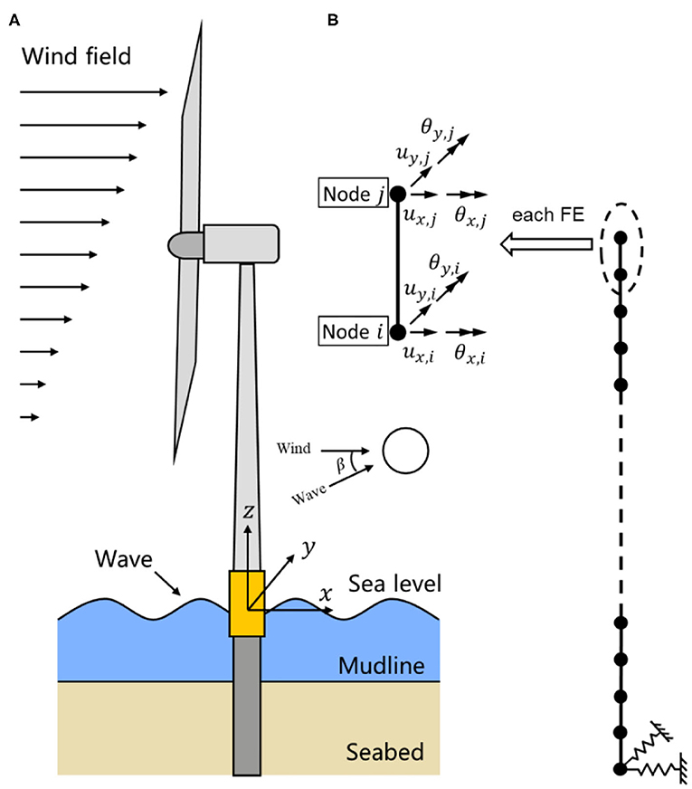
Figure 1. Monopile offshore wind turbine and its FE model. (A) Overview of the monopile offshore wind turbine. (B) FE model of the tower.

FIGURE 2

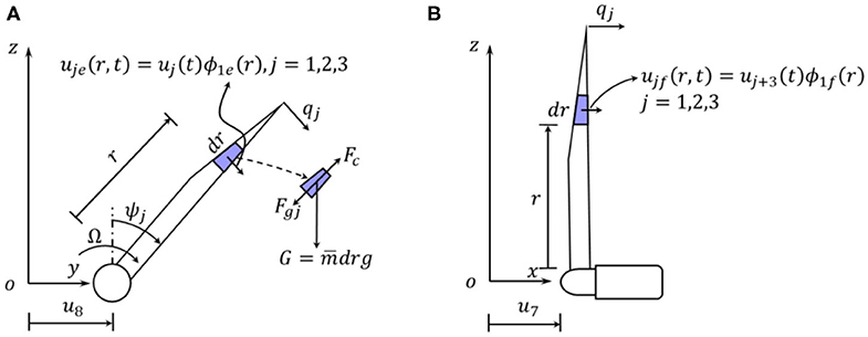
Figure 2. Degrees-of-freedom of the rotor blades. (A) Blade in-plane movement. (B) Blade out-of-plane movement.

FIGURE 3

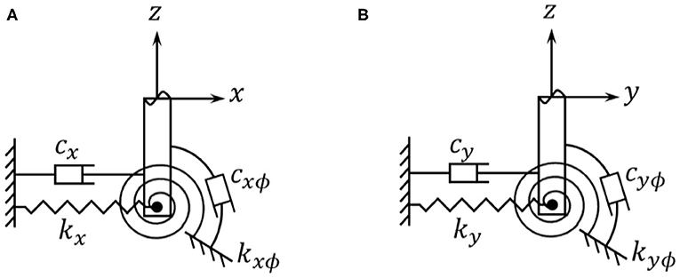
Figure 3. Simplified foundation model of the offshore wind turbine. (A) Foundation model in xz plane. (B) Foundation model in yz plane.

In this study, the modeling of the aerodynamic and hydrodynamic components of OWT follows the procedure described in Sun and Jahangiri (2018); Sun (2018a); Sun (2018b). The tower, however, is modeled by FE method with physical movements as the DOFs instead of modal coordinates—the major bending modes in x and y directions adopted in Sun and Jahangiri (2018); Sun (2018a); Sun (2018b). The equations of motion of the OWT are established accordingly. The derivation details are shown in the Sections FE Model for Tower Including Foundation, Kinetic Energy, Potential Energy, Loads on OWT.

FE Model for Tower Including Foundation

In actual RTHS implementation, usually the tower structure of the OWT is built in wave tank facility in reduced scale. In this concept study, all the components of the RTHS, including the experimental component (tower structure), are simulated numerically. As shown in Figure 1B, the entire tower of the OWT, including the tower structure above the MSL and below until seabed (also called the wet section), is modeled together as one tower model using two-node 3D elastic beam elements. Each node contains four DOFs: two translations (u_x, u_y) and two rotations (θ_x, θ_y) with respect to the x and y axis. The torsional behavior and axial deformation of the tower are ignored in this study. Assuming modal damping, the formulation of the mass M_tow, stiffness K_tow, and damping C_tow matrices can be found in standard texts (Przemieniecki, 1968; Craig and Kurdila, 2006) and hence are not repeated here. The pile is modeled as part of the tower structure extended to the seabed. Once the global mass, stiffness, and damping matrices of the tower are assembled, they are further modified by adding the stiffness (k_x, k_y, k_xϕ, and k_yϕ) and damping (c_x, c_y, c_xϕ, and c_yϕ) terms from the foundation model shown in Figure 3 to the corresponding DOFs. With the FE model of the tower established, the kinetic energy T_tow and potential energy V_tow of the tower can be expressed as

$\begin{array}{ll}{T}_{tow}=\frac{1}{2}{\text{v}}_{tow}^T{\text{M}}_{tow}{\text{v}}_{tow}& (2)\end{array}$

and

$\begin{array}{ll}{V}_{tow}=\frac{1}{2}{\text{u}}_{tow}^T{\text{K}}_{tow}{\text{u}}_{tow}& (3)\end{array}$

where M_tow and K_tow are the mass matrix and stiffness matrix; u_tow and v_tow are the displacement and velocity response vectors of the DOFs of the tower; Superscript “T” indicates transpose operation. It is noted that u₇ and u₈ are included in the vector u_tow too.

Kinetic Energy

Based on Figures 1, 2, the absolute velocity of the nacelle (and the hub) v_nac is expressed as

$\begin{array}{ll}{v}_{nac}(r,t)=\sqrt{{\stackrel{\bullet }{u}}_7^2+{\stackrel{\bullet }{u}}_8^2}& (4)\end{array}$

Consider an infinitesimal unit dr of the jth blade in Figure 2, its movements (x_r,j, y_r,j, z_r,j) in the xyz coordinate system can be expressed as (j = 1, 2, 3)

$\begin{array}{ll}{x}_{r,j}=u_7+u_{jf}=u_7+u_{j+3}{\varphi }_{1f}& (5)\end{array}$

$\begin{array}{l}{y}_{r,j}=u_8+rsin{\psi }_j+u_{je}cos{\psi }_j=u_8+rsin{\psi }_j\\ +u_j{\varphi }_{1e}cos{\psi }_j& (6)\end{array}$

$\begin{array}{ll}{z}_{r,j}=rcos{\psi }_j-u_{je}sin{\psi }_j=rcos{\psi }_j-u_j{\varphi }_{1e}sin{\psi }_j& (7)\end{array}$

Taking the derivative with respect to time, the magnitude of the absolute velocity of the unit dr of the jth blade v_b,j in Figure 2 is

$\begin{array}{ll}{v}_{b,j}(r,t)=\sqrt{{\left({\stackrel{·}{x}}_{r,j}\right)}^2+{\left({\stackrel{·}{y}}_{r,j}\right)}^2+{\left({\stackrel{·}{z}}_{r,j}\right)}^2}& (8)\end{array}$

Therefore, the total kinetic energy T of the OWT is given as

$\begin{array}{l}T=\frac{1}{2}{\displaystyle \sum _{j=1}^3{\displaystyle {\int }_0^R\overline{m}{v}_{b,j}^2\left(r,t\right)dr}}+\frac{1}{2}\left(M_{nac}+M_{hub}\right)v_{nac}^2+T_{tow}\\ =\frac{1}{2}{\displaystyle \sum _{j=1}^3{\displaystyle {\int }_0^R\overline{m}{v}_{b,j}^2\left(r,t\right)dr}}\\ +\frac{1}{2}{\left[\begin{array}{c}{\dot{u}}_7\\ {\dot{u}}_8\end{array}\right]}^T\left[\begin{array}{cc}{M}_{nac}+M_{hub}& 0\\ 0& M_{nac}+M_{hub}\end{array}\right]\left[\begin{array}{c}{\dot{u}}_7\\ {\dot{u}}_8\end{array}\right]\\ +\frac{1}{2}{v}_{tow}^T{M}_{tow}{v}_{tow}& (9)\end{array}$

where R denotes the length of the blade; M_nac and M_hub are the mass for the nacelle and hub, respectively; $\overline{m}$ is the mass density per length of the blade.

Potential Energy

The total potential energy of the blades V_b is calculated considering the strain energy due to bending and the stiffening effects due to centrifugal force and gravity. It is expressed as Sun and Jahangiri (2018).

$\begin{array}{l}{V}_b=\frac{1}{2}{\displaystyle \sum _{j=1}^3[\left(k_{eg}+k_{ge,eg}-k_{gr,eg}\cos {\psi }_j\right)u_j^2}\\ +\left(k_{fp}+k_{ge,fp}-k_{gr,fp}\cos {\psi }_j\right)u_{j+3}^2]& (10)\end{array}$

where the bending stiffness in edge and flap direction, k_eg and k_fp, are expressed as,

$\begin{array}{l}{k}_{eg}={\displaystyle {\int }_0^{R}E{I}_{eg}\left(r\right){\left({\varphi }_{1e}″\right)}^{2}dr}\\ k_{fp}={\displaystyle {\int }_0^{R}E{I}_{fp}\left(r\right){\left({\varphi }_{1f}″\right)}^{2}dr}\end{array}$

the tension stiffening geometric stiffness in edge and flap direction due to centrifugal force, k_ge,eg and k_ge,fp, are expressed as,

$\begin{array}{l}{k}_{ge,eg}={\Omega }^2{\displaystyle {\int }_0^R{\displaystyle {\int }_r^R\left[\overline{m}\left(\xi \right)\xi d\xi \right]}}{\left({\varphi }_{1e}\prime \right)}^{2}dr\\ k_{ge,fp}={\Omega }^2{\displaystyle {\int }_0^R{\displaystyle {\int }_r^R\left[\overline{m}\left(\xi \right)\xi d\xi \right]}}{\left({\varphi }_{1f}\prime \right)}^{2}dr\end{array}$

the tension stiffening geometric stiffness in edge and flap direction due to gravity, k_gr,eg and k_gr,fp, are expressed as,

$\begin{array}{l}{k}_{gr,eg}=g{\displaystyle {\int }_0^R{\displaystyle {\int }_r^R\left[\overline{m}\left(\xi \right)d\xi \right]}}{\left({\varphi }_{1e}\prime \right)}^{2}dr\\ k_{gr,fp}=g{\displaystyle {\int }_0^R{\displaystyle {\int }_r^R\left[\overline{m}\left(\xi \right)d\xi \right]}}{\left({\varphi }_{1f}\prime \right)}^{2}dr\end{array}$

where I_eg and I_fp are the moment of inertia in the edgewise and flapwise direction, g is the gravitational acceleration; the superscripts “′” and “″” denote the first and second order derivatives with respect to the blade length R. Therefore, the total potential energy V of the OWT is.

$\begin{array}{ll}V=V_b+V_{tow}=V_b+\frac{1}{2}{\text{u}}_{tow}^T{\text{K}}_{tow}{\text{u}}_{tow}& (11)\end{array}$

Loads on OWT

This section presents the derivation of wind, wave, and damping forces based on the principle of virtual work and FE method.

Wind Loading

The generation of the wind field follows IEC 61400-1 standard (Iec, 2005) using the Kaimal spectral model, with the length of roughness is set equal to 0.03. The associated coherence function is defined as,

$\begin{array}{ll}\text{Coh}\left(i,j;f\right)=exp\left(-a\sqrt{{\left(\frac{fL}{{\overline{V}}_{hub}}\right)}^2+{\left(\frac{0.12L}{L_c}\right)}^2}\right)& (12)\end{array}$

where a = 12, L_c = 340.2 m are adopted in this study. During implementation, a three dimensional wind field profile covering the domain of the rotor disk is generated using the TurbSim program (Jonkman and Kilcher, 2012). A MATLAB code is developed to map the generated wind field onto each spanwise elements of the rotating blades to apply the BEM theory.

In this study, the BEM theory (Hansen, 2015) is applied to calculate the aerodynamic loads on the rotor blades. Figure 4 shows a blade element with the velocities and angles that determine the aerodynamic loads on the element. The angle of attack is denoted as α; c is the local chord length; θ is the sum of the local pitch angle and the twist of the blade element, which are determined by the blade profile; the relative velocity V_rel is a combination of the axial velocity V_∞(1 − a) and the tangential velocity Ωr(1 + a′) at the rotor plane, where V_∞ is the flow velocity; r is the radial distance from the blade element to the rotor center; a and a′ are the axial and tangential induction factors, respectively. The lift and drag forces are projected to the directions normal to and tangential to the rotor plane to obtain the aerodynamic forces (per length) normal to the rotor plane p_N and tangential to the rotor plane p_T, as shown in the Equation (13),

$\begin{array}{l}{p}_N=Lcos\varphi +Dsin\varphi =\frac{1}{2}{\rho }_A{V}_{rel}^{2}c(C_{l}cos\varphi +C_{d}sin\varphi )\\ p_T=Lsin\varphi -Dcos\varphi =\frac{1}{2}{\rho }_A{V}_{rel}^{2}c(C_{l}sin\varphi -C_{d}cos\varphi )& (13)\end{array}$

where ρ_A is the air density; the lift and drag coefficients C_l and C_d can be determined from a given blade profile.

FIGURE 4

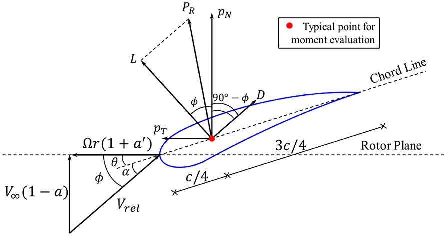
Figure 4. Blade element velocities, flow angles, and aerodynamic loads.

In practice, because the induction factors a and a′ are not known, an iterative procedure is required to implement the BEM theory. In this study, a MATLAB code is developed to calculate the time series of p_N and p_T based on an algorithm proposed in Sun (2018a). Prandtl's model and Glauert correction are considered in the MATLAB code to account for tip- and hub-loss. After the aerodynamic forces are determined, the principle of virtual work is applied to calculate the generalized aerodynamic loads on the OWT model.

Under p_N and p_T, the virtual work δW_wind done by external wind load is expressed as,

$\begin{array}{l}\delta W_{wind}={\displaystyle \sum _{j=1}^3[{\displaystyle {\int }_0^R{p}_{Tj}\left(r,t\right)\left({\varphi }_{1e}\delta u_j+\delta u_8\cos {\psi }_j\right)dr}}\\ +{\displaystyle {\int }_0^R{p}_{Nj}\left(r,t\right)\left({\varphi }_{1f}\delta u_{j+3}+\delta u_7\right)dr}]& (14)\end{array}$

where p_Nj and p_Tj denote the normal and tangential aerodynamic forces (per length) p_N and p_T acting on the jth blade. It is noted that the work done by the aerodynamic load acting on the DOFs of the tower is shown to be zero, except at the tip of the tower where the nacelle (and the hub) is located, i.e., u₇ and u₈.

Wave and Current Loading

In this study, the JONSWAP wave spectrum is adopted to characterize wave climate. Based on the spectral representation method and linear wave theory, the random wave surface elevation η_w, current velocity ${\stackrel{\bullet }{u}}_w$, and acceleration ü_w can be generated as,

$\begin{array}{ll}{\eta }_w(x,t)={\displaystyle \sum _{j=1}^{\text{N}}}{A}_{j}cos\left(2\pi f_{j}t-k_{j}x+{\varphi }_j\right)& (15)\end{array}$

$\begin{array}{r}{\stackrel{\bullet }{u}}_w(x,z,t)={\displaystyle \sum _{j=1}^{\text{N}}}\left(2\pi f_j\right)A_j\frac{cosh[k_j(z+H_w)]}{sinh\left(k_j{H}_w\right)}\\ cos\left(2\pi f_{j}t-k_{j}x+{\varphi }_j\right)& (16)\end{array}$

$\begin{array}{r}{\ddot{u}}_w(x,z,t)=-{\displaystyle \sum _{j=1}^{\text{N}}}{\left(2\pi f_j\right)}^2{A}_j\frac{cosh[k_j(z+H_w)]}{sinh\left(k_j{H}_w\right)}\\ sin\left(2\pi f_{j}t-k_{j}x+{\varphi }_j\right)& (17)\end{array}$

where Δf = f_cut/N denotes the resolution of the frequency domain; N, usually a large number, indicates the number of segments that the frequency domain is divided into; and f_cut is the upper cut-off frequency for wave spectrum S; $A_j=2\sqrt{S(f_j)\Delta f}$ and f_j = j·Δf, j = 1, …, N; S is the JONSWAP wave spectrum (Dnvgl, 2010); ϕ_j is the generated random phase angle uniformly distributed from 0 to 2π; H_w denotes water depth; k_j represents wave number, which is related to f_j by the dispersion equation (Faltinsen, 1990)

$\begin{array}{ll}{\left(2\pi f_j\right)}^2=g{k}_{j}tanh(k_j{H}_w)& (18)\end{array}$

In Figure 5, the time history (for 200 s) and the spectrum of a generated random wave with the setting of wave peak period T_p = 10 s, significant wave height H_s = 3m, water depth H_w = 17.5m, number of segments N = 2, 000 are generated and compared with the target JONSWAP spectrum. The close match indicates the generated wave achieves the desired wave climate and can be used for load evaluation.

FIGURE 5

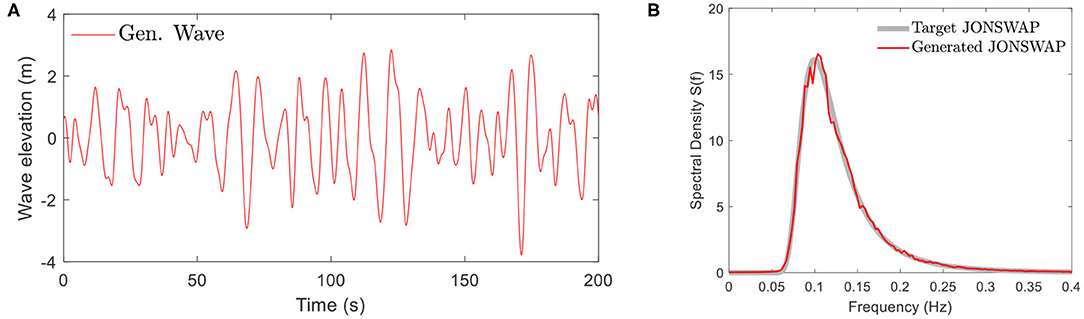
Figure 5. Generated wave (T_p = 10 s, H_s = 3m, H_w = 17.5m, N = 2000). (A) Time history of the generated wave elevation. (B) Spectrum of the generated wave.

With the current velocity ${\stackrel{\bullet }{u}}_w$ and acceleration ü_w obtained from Equations (16) and (17), the hydrodynamic forces exerted on a unit length of a pile can be evaluated using Morison's equation (Morison et al., 1950).

$\begin{array}{ll}F=F_d+F_a=\frac{1}{2}{\rho }_{w}D{C}_d{\stackrel{\bullet }{u}}_w\left|{\stackrel{\bullet }{u}}_w\right|+\frac{1}{4}{\rho }_w\pi D^2{C}_m{\ddot{u}}_w& (19)\end{array}$

Where $F_d=\frac{1}{2}{\rho }_{w}D{C}_d{\stackrel{\bullet }{u}}_w\left|{\stackrel{\bullet }{u}}_w\right|$ denotes the drag orce (per length) and $F_a=\frac{1}{4}{\rho }_w\pi D^2{C}_m{\ddot{u}}_w$ denotes the inertia force (per length); ρ_w is the density of the fluid (${\rho }_w=1,025kg/m^3$ is adopted in this study); D is the diameter of the pile section; C_d and C_m are the drag and inertial coefficients (C_d = 1.2, C_m = 2.0 are adopted in this study). The virtual work δW_wave done by the hydrodynamic forces along the tower including the monopile under MSL can be expressed as,

$\begin{array}{l}\delta W_{wave}={\displaystyle {\int }_{-H_w}^0}F\left[\left(cos\beta \delta u_x+sin\beta \delta u_y\right)\right]\\ \approx {\displaystyle \sum _{i=1}^{{\text{N}}_{\text{w}}}}\delta {\text{u}}_{tow,i}^T{\text{F}}_{wave,i}& (20)\end{array}$

where δu_x and δu_y indicate the virtual displacement along x and y directions, respectively. The last approximation in Equation (20) is based on work-equivalent nodal force using the FE model established in Section FE Model for Tower Including Foundation. N_w indicates the total number of elements that are below MSL; F_{wave, i} and δu_{tow, i} are the work-equivalent nodal force vector and virtual displacement vector of the ith element of the tower FE model, respectively. It is noted that δW_wave does not involve the DOFs above the MSL.

Damping Load

Modal damping is assumed for both the blades and the tower. The virtual work done by the damping force is given as,

$\begin{array}{l}\delta W_{damping}=\delta W_{damping,bl}+\delta W_{damping,tow}\\ =-{\displaystyle \sum _{j=1}^3\left(c_{bj,eg}{\dot{u}}_j\delta u_j+c_{bj,fp}{\dot{u}}_{j+3}\delta u_{j+3}\right)}\\ -{\left[\begin{array}{c}\delta u_7\\ \delta u_8\end{array}\right]}^T\left[\begin{array}{cc}{c}_{aero,x}& 0\\ 0& c_{aero,y}\end{array}\right]\left[\begin{array}{c}{\dot{u}}_7\\ {\dot{u}}_8\end{array}\right]-{\left(\delta u_{tow}\right)}^T{C}_{tow}{v}_{tow}& (21)\end{array}$

where c_{bj, eg} and c_{bj, fp} are the edgewise and flapwise modal damping coefficients of the jth blade; c_{aero, x} and c_{aero, y} are the aerodynamic damping coefficients of the nacelle in x and y directions, respectively; C_tow is the modal damping matrix of the FE model of the tower.

Equations of Motion of OWT

With the kinetic energy, potential energy, and the forces obtained, the equations of motion of the monopile OWT can be obtained using the Euler-Lagrange equation as follows,

$\begin{array}{ll}\frac{d}{dt}\frac{\partial T}{\partial {\stackrel{\bullet }{u}}_i}-\frac{\partial T}{\partial u_i}+\frac{\partial V}{\partial u_i}=F_i& (22)\end{array}$

where the kinetic energy T and potential energy V can be obtained from Equation (9) and Equation (11), respectively; u_i indicates each DOF of the FE model of the tower; the corresponding forcing term F_i can be obtained by,

$\begin{array}{ll}{F}_i=\frac{\partial (\delta W)}{\partial (\delta u_i)}=\frac{\partial \left(\delta W_{wind}+\delta W_{wave}+\delta W_{damping}\right)}{\partial (\delta u_i)}& (23)\end{array}$

with δW_wind, δW_wave, and δW_damping obtained from Equations (14), (20), and (21).

After collecting the terms in Equation (22), the following equations of motion can be obtained,

$\begin{array}{ll}\text{M}\ddot{\text{u}}+\text{C}\stackrel{\bullet }{\text{u}}+Ku=\text{F}& (24)\end{array}$

where $u_{\text{N}}={\left[\begin{array}{c}{u}_1{u}_2{u}_3{u}_4{u}_5{u}_6{u}_{tow}^T\end{array}\right]}^T$; the corresponding mass matrix M, damping matrix C, stiffness matrixK, and force vector F are listed in the Appendix.

Proposed Real-Time Hybrid Simulation Framework

A RTHS framework is proposed in this section to study the structural behavior of the monopile OWT shown in Figure 1A. Its details, including the framework descript, possible scaling laws applied, and error contributors are explained in Section. Proposed Real-Time Hybrid Simulation Framework.

Framework Description

The proposed RTHS platform is shown in Figure 6. In this RTHS platform, the numerical component contains the rotor blades and aerodynamic loads; the experimental component contains the tower structure (including the nacelle, hub, and foundation) along with the hydrodynamic loading effects provided by wave tank and necessary hardware (actuators and sensors). It is noted that, the numerical component is simulated under full-scale, and the experimental component is tested in reduced scale. The two components are interfaced through the displacement DOFs (u₇ and u₈) at the top of the tower. This RTHS framework directly resolves the Froude-Reynold scaling conflict by applying full-scale aerodynamic simulation in the numerical component, and meanwhile it can preserve the complex hydrodynamic behaviors in the wave tank facility at a reduced scale, including soil-structure interaction and wave-current interaction. In this concept study, to assess the feasibility of the proposed RTHS framework and identify possible contributors that may impact the RTHS performance, a “virtual” RTHS is established through numerical simulation of both the numerical and experimental components.

FIGURE 6

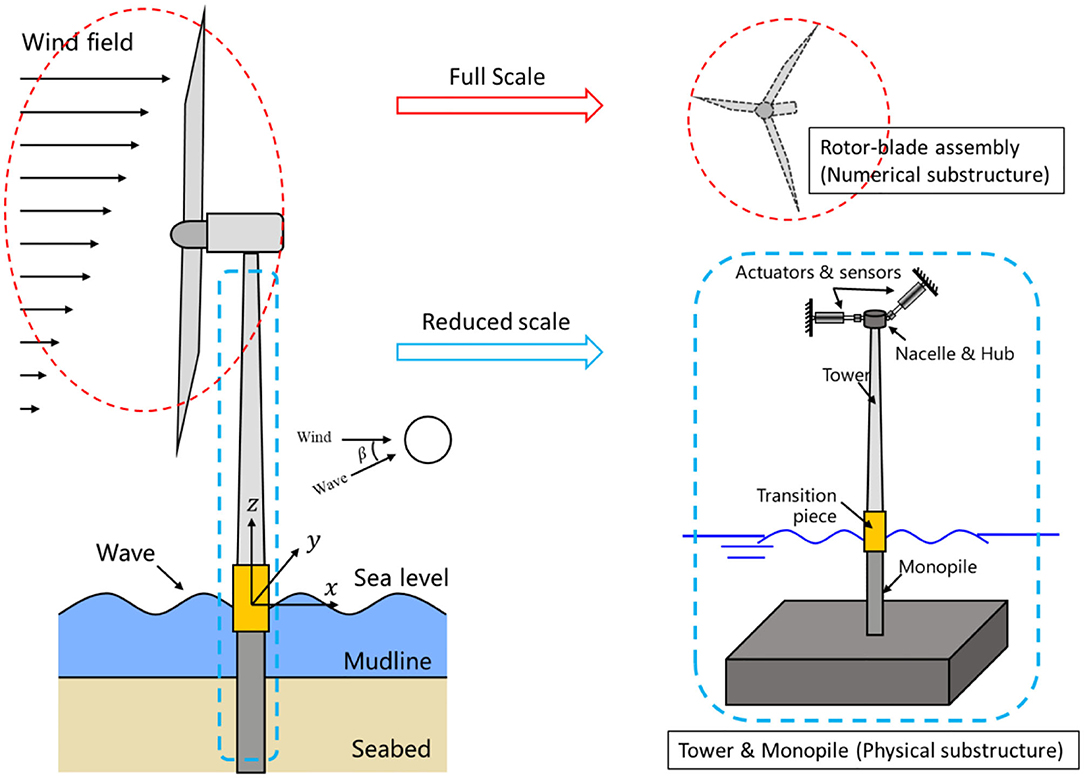
Figure 6. Monopile OWT and its RTHS components.

To explain, the displacement vector of the entire OWT, u, defined in Equation (24) is partitioned based on the proposed RTHS framework as,

$\begin{array}{ll}u={\left[\begin{array}{ccccccc}{u}_1& u_2& u_3& u_4& u_5& u_6& u_{tow}^{\text{T}}\end{array}\right]}^T={\left[\begin{array}{ccc}{u}_{\text{N}}^{\text{T}}& u_{\text{I}}^{\text{T}}& u_{\text{E}}^{\text{T}}\end{array}\right]}^{\text{T}}& (25)\end{array}$

where ${\text{u}}_{\text{N}}={\left[\begin{array}{c}{u}_1{u}_2{u}_3{u}_4{u}_5{u}_6\end{array}\right]}^T$, ${\text{u}}_{\text{I}}={\left[\begin{array}{c}{u}_7{u}_8\end{array}\right]}^T$, and u_E is the tower displacement vector u_tow excluding the DOFs of u_I. The subscripts “I”, “N”, and “E” indicate the DOFs are related to the interfacing system, numerical component, and experimental component of the proposed RTHS framework, respectively. Based on the partition shown in Equation (25), the equations of motion, Equation (24), can be written into the partitioned formulation as,

$\begin{array}{l}\left[\begin{array}{ccc}{M}_{\text{NN}}& M_{\text{NI}}& 0\\ M_{\text{IN}}& M_{\text{II}}^{\text{N}}+M_{\text{II}}^{\text{E}}& M_{\text{IE}}\\ 0& M_{\text{EI}}& M_{\text{EE}}\end{array}\right]\left[\begin{array}{c}{\ddot{u}}_{\text{N}}\\ {\ddot{u}}_{\text{I}}\\ {\ddot{u}}_{\text{E}}\end{array}\right]\\ +\left[\begin{array}{ccc}{C}_{\text{NN}}& C_{\text{NI}}& 0\\ C_{\text{IN}}& C_{\text{II}}^{\text{N}}+C_{\text{II}}^{\text{E}}& C_{\text{IE}}\\ 0& C_{\text{EI}}& C_{\text{EE}}\end{array}\right]\left[\begin{array}{c}{\dot{u}}_{\text{N}}\\ {\dot{u}}_{\text{I}}\\ {\dot{u}}_{\text{E}}\end{array}\right]\\ +\left[\begin{array}{ccc}{K}_{\text{NN}}& K_{\text{NI}}& 0\\ K_{\text{IN}}& K_{\text{II}}^{\text{N}}+K_{\text{II}}^{\text{E}}& K_{\text{IE}}\\ 0& K_{\text{EI}}& K_{\text{EE}}\end{array}\right]\left[\begin{array}{c}{u}_{\text{N}}\\ u_{\text{I}}\\ u_{\text{E}}\end{array}\right]=\left[\begin{array}{c}{F}_{\text{N}}\\ F_{\text{I}}^{\text{N}}+F_{\text{I}}^{\text{E}}\\ F_{\text{E}}\end{array}\right]& (26)\end{array}$

The subscripts are defined in the same manner as in Equation (25). The superscripts “E” and “N” indicate the term originates from the experimental component or from the numerical component. The detailed expressions for each term are listed in the Appendix.

Based on Equation (26), the equation of motion for the numerical component [1^st block row in Equation (26)] of the RTHS framework can be determined as

$\begin{array}{ll}{\text{M}}_{\text{NN}}{\ddot{\text{u}}}_{\text{N}}+{\text{C}}_{\text{NN}}{\stackrel{\bullet }{\text{u}}}_{\text{N}}+{\text{K}}_{\text{NN}}{\text{u}}_{\text{N}}={\text{F}}_{\text{N}}-{\text{f}}_{\text{I}}^{\text{N}}& (27)\end{array}$

where ${\text{f}}_{\text{I}}^{\text{N}}$ indicates the interface force acting on the numerical component. It can be computed as

$\begin{array}{ll}{\text{f}}_{\text{I}}^{\text{N}}={\text{M}}_{\text{NI}}{\ddot{\text{u}}}_{\text{I}}+{\text{C}}_{\text{NI}}{\stackrel{\bullet }{\text{u}}}_{\text{I}}+{\text{K}}_{\text{NI}}{\text{u}}_{\text{I}}={\text{M}}_{\text{NI}}{\ddot{\text{u}}}_{\text{I}}& (28)\end{array}$

The last equality in Equation (28) holds because C_NI = 0 and K_NI = 0 (see Appendix).

Similarly, the equation of motion for the experimental component [2^nd and 3^rd block rows in Equation (26)] of the RTHS framework can be determined as

$\begin{array}{l}\left[\begin{array}{cc}{M}_{\text{II}}^{\text{E}}& M_{\text{IE}}\\ M_{\text{EI}}& M_{\text{EE}}\end{array}\right]\left[\begin{array}{c}{\ddot{u}}_{\text{I}}\\ {\ddot{u}}_{\text{E}}\end{array}\right]+\left[\begin{array}{cc}{C}_{\text{II}}^{\text{E}}& C_{\text{IE}}\\ C_{\text{EI}}& C_{\text{EE}}\end{array}\right]\left[\begin{array}{c}{\dot{u}}_{\text{I}}\\ {\dot{u}}_{\text{E}}\end{array}\right]+\left[\begin{array}{cc}{K}_{\text{II}}^{\text{E}}& K_{\text{IE}}\\ K_{\text{EI}}& K_{\text{EE}}\end{array}\right]\left[\begin{array}{c}{u}_{\text{I}}\\ u_{\text{E}}\end{array}\right]\\ =\left[\begin{array}{c}{F}_{\text{I}}^{\text{E}}\\ F_{\text{E}}\end{array}\right]+\left[\begin{array}{c}{F}_{\text{I}}^{\text{N}}-f_{\text{I}}^{\text{E}}\\ 0\end{array}\right]& (29)\end{array}$

where ${\text{f}}_{\text{I}}^{\text{E}}$ indicates the interface force acting on the experimental component. It can be computed as

$\begin{array}{l}{\text{f}}_{\text{I}}^{\text{E}}={\text{M}}_{\text{IN}}{\ddot{\text{u}}}_{\text{N}}+{\text{C}}_{\text{IN}}{\stackrel{\bullet }{\text{u}}}_{\text{N}}+{\text{K}}_{\text{IN}}{\text{u}}_{\text{N}}+{\text{M}}_{\text{II}}^{\text{N}}{\ddot{\text{u}}}_{\text{I}}+{\text{C}}_{\text{II}}^{\text{N}}{\stackrel{\bullet }{\text{u}}}_{\text{I}}+{\text{K}}_{\text{II}}^{\text{N}}{\text{u}}_{\text{I}}\\ ={\text{M}}_{\text{IN}}{\ddot{\text{u}}}_{\text{N}}+{\text{C}}_{\text{IN}}{\stackrel{\bullet }{\text{u}}}_{\text{N}}+{\text{K}}_{\text{IN}}{\text{u}}_{\text{N}}+{\text{M}}_{\text{II}}^{\text{N}}{\ddot{\text{u}}}_{\text{I}}+{\text{C}}_{\text{II}}^{\text{N}}{\stackrel{\bullet }{\text{u}}}_{\text{I}}& (30)\end{array}$

The last equality in Equation (30) holds because ${\text{K}}_{\text{II}}^{\text{N}}=0$ (see Appendix). In addition, if sufficient amount of mass can be added to the experimental component to include the mass effect from the nacelle and rotor systems, i.e., ${\text{M}}_{\text{II}}^{\text{N}}$, then ${\text{M}}_{\text{II}}^{\text{N}}{\ddot{\text{u}}}_{\text{I}}$ can be removed from Equation (30) as it will be naturally considered during the testing of experimental component.

Based on the numerical and experimental components defined in Figure 6, the procedure for RTHS using wave tank facility can be extracted from Equations (27)~(30). To summarize, the numerical component takes the measurement of ${\ddot{\text{u}}}_{\text{I}}$ during the test to compute ${\text{f}}_{\text{I}}^{\text{N}}$ [Equation. (28)]. The response of numerical component, u_N, under the combined action of aerodynamic load F_N and ${\text{f}}_{\text{I}}^{\text{N}}$, is determined through numerical integration by solving Equation (27). The solved responses (u_N, ${\stackrel{\bullet }{\text{u}}}_{\text{N}}$, and ${\ddot{\text{u}}}_{\text{N}}$) are used to compute ${\text{f}}_{\text{I}}^{\text{E}}$ (Equation 30). In wave tank facility, ${\text{f}}_{\text{I}}^{\text{E}}$ combined with the aerodynamic force ${\text{F}}_{\text{I}}^{\text{N}}$ are applied to the OWT specimen via actuators, while the force vector ${\left[\begin{array}{c}{({\text{F}}_{\text{I}}^{\text{E}})}^T{({\text{F}}_E)}^T\end{array}\right]}^T$is generated via wavemaker. Then, the induced response (${\ddot{\text{u}}}_{\text{I}}$) is measured through sensors and fed to the numerical component to close the loop. A block diagram describing this process is provide in Figure 7.

FIGURE 7

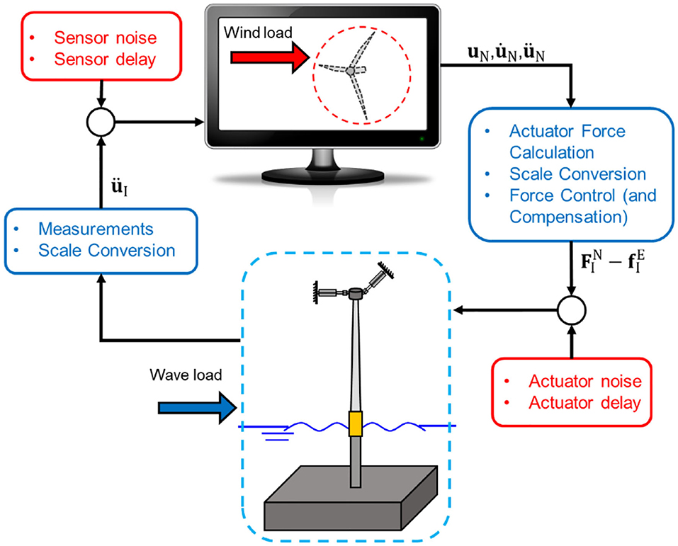
Figure 7. Block diagram of the proposed RTHS framework.

Scaling Laws

In the proposed RTHS framework (Figure 6), the scaling conflict is avoided because the aerodynamic effects are simulated in full-scale, which is separated from the hydrodynamic effects produced in wave tank facility in reduced scale. So far, most of the existing scaled wave tank tests adopts Froude scaling, because the Froude number, Fr, defined in Equation (31) below, characterizes the gravitational effect which is dominating in problems with free surface waves.

$\begin{array}{ll}Fr=V/\sqrt{gL}& (31)\end{array}$

where V is the wave celerity or propagation speed, g is the gravitational acceleration, and L is the characteristic length. However, hydrodynamic effects due to water waves are not the only dynamic effects need to be considered in the RTHS tests. The elastic effect due to slender specimen deformation also needs to be considered. Following the Froude scaling, it can be shown that the consistent scaling to preserve the similitude in structural modal information (natural frequencies and mode shapes) is (Martin, 2011; Bredmose et al., 2012)

$\begin{array}{ll}{\lambda }_{EI}={\lambda }_{\rho }{\lambda }_L^5& (32)\end{array}$

where λ_EI, λ_ρ, and λ_L are the scaling factor of bending stiffness (EI), density (ρ), and length (L), between the model and the prototype. It is noted that (Equation 32) implies that if the density of the material stays unchanged (λ_ρ = 1), the elastic modulus E needs to be modified. This requirement is usually difficult to achieve directly. Often for the OWT tower, it is sufficient that the bending stiffness EI scales correctly, which provides some freedom in the model design. Therefore, the combination of material density, stiffness, and geometry are usually tuned together to achieve the scaling goal. This method, although challenging, has been applied in OWT wave tank studies (Martin, 2011; Martin et al., 2014).

In this study, several alternatives have been considered in addition to the above Froude scaling law. In earthquake engineering, Cauchy scaling combined with Froude scaling are often considered in designing scaled models for dynamic testing. Cauchy scaling preserves the Cauchy number, Ca, defined in Equation (33), which is important in characterizing the deformation of the specimen.

$\begin{array}{ll}Ca=\rho V^2/E& (33)\end{array}$

With the condition λ_E = λ_ρλ_L, Froude and Cauchy similitudes are simultaneous. It implies that if the same material is used for both prototype and model with λ_E = 1, the density of the specimen needs to be increased. Usually added artificial masses are distributed to the model specimen to achieve that and minimize the change in mass distribution. However, when applying this simultaneous Fr-Ca scaling law, the hydrodynamic effects are distorted, because water usually is the only liquid considered in wave tank facilities. Under the Fr-Ca similitude, the proper scaling factor for force acting on the OWT ${\lambda }_{tf}={\lambda }_L^2$. But with water used as the testing fluid, the scaling factor for hydrodynamic force induced by wave and current is, ${\lambda }_{hf}={\lambda }_L^3\ne {\lambda }_{tf}$, which causes distortion in hydrodynamic force scaling. To consider the impacts of possible scaling laws on the proposed RTHS, a total of three scaling laws are considered in this study:

• Froude scaling with λ_ρ = 1. In this case, all terms are properly scaled but it poses a challenge to the model construction in preserving the similitude in bending stiffness;

• Conventional Fr-Ca scaling, which induces distorted hydrodynamic force induced from the wave tank;

• Fr-Ca scaling with increased wave amplitude. By increasing the amplitude of the generated wave by a factor of $\sqrt{1/{\lambda }_L}$, the drag force F_d in Equation (19) can be properly scaled with a factor of ${\lambda }_L^2$, matching the requirement from the OWT. However, the inertia force F_a is still distorted under this scaling law.

The last two of the scaling laws both are derived from Fr-Ca scaling. A systematic way of model construction is the advantage in them, comparing to the Froude scaling. The trade-off is they both suffer from distorted hydrodynamic effects. One of the goals in this study is to examine how these scaling laws impact the error in the proposed RTHS framework. Other options have also been considered in the early stage of this study:

• Fr-Ca scaling with increased depth by a factor of 1/λ_L. In this case, the wet section of the tower (z ∈ [−H_w, 0]) is effectively unscaled, then the similitude of hydrodynamic forces generated on the specimen are preserved. But it is infeasible for wave tank facility to offer such a depth to study OWT. In addition, the design of the unscaled section needs to be adjusted to preserve the similitude in bending stiffness and mass.

• Fr-Ca scaling with increased wave amplitude by a factor of 1/λ_L. In this case, the amplitude of the generated wave is effectively unscaled. The inertia force F_a is properly scaled with a factor of ${\lambda }_L^2$, but the drag force F_d is distorted. This option is infeasible due to its high demand in the wavemaker.

• Froude scaling with λ_ρ = 1 and no further adjustment for the tower geometry, i.e., no added mass nor a matching bending stiffness EI. In this case, the hydrodynamic effects from the wave tank are properly scaled, but the modal properties of the OWT is distorted which causes significant response error.

These three options all have been rejected due to issues in their feasibility or accuracy.

Error Contributors

In RTHS, experimental errors accumulate in real-time closed loop through the numerical integration scheme due to control and measurement discrepancies. It is known that delays and noises in the interfacing actuator and sensor systems are the main contributors to the above errors, as they tend to bring destabilizing effect into RTHS, causing large experimental error or even failure (Christenson et al., 2014; Maghareh et al., 2014; Hayati and Song, 2017). Such destabilizing effect is more pronounced in reduced scaled model testing than in full-scale, because the frequency of interest is amplified according to scaling process (Hayati and Song, 2018; Wu and Song, 2019). In addition, the impact of modeling choices (e.g., scaling laws, wave heights, and misalignment angles) on errors are also studied to guide future specimen designs.

In this study, to evaluate the feasibility and assess the performance of the proposed RTHS framework, noises, and delays are considered as the primary error contributors and modeled into the RTHS. As a concept study, the hardware implementation issues of sensors and actuators are out of the current scope. In Figure 7, a block diagram is provided to illustrate the general RTHS process described in Section. Framework Description. The noises and delays considered are the actuator noise, actuator delay, sensor noise, and sensor delay, which are also shown in Figure 7. The details of how the delays and noises are generated can be found in Section. Case I: Delay and Section. Case II: Noise, respectively. In addition, the other possible error contributors considered in this study are the scaling laws, misalignment angle β and the significant wave height H_s.

Numerical Study

A concept study is carried out to assess the feasibility and identify the impact of the selected contributors on the performance of the proposed RTHS. The details and results for the study are described in Section. Numerical Study.

System Parameters

The National Renewable Energy Lab (NREL) 5-MW reference wind turbine (Jonkman et al., 2009) is used in this study. Details of the modeling parameters are presented in Table 1.

TABLE 1

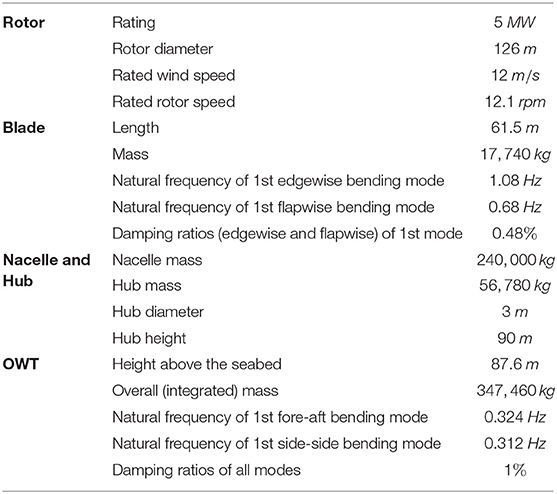
Table 1. Modeling parameters of the NREL 5-MW reference wind turbine.

As indicated in Figure 3, soil effects are considered using linear springs and dashpots. According to Carswell et al. (2015); Sun and Jahangiri (2018), the values for the spring stiffness are chosen as $k_x=k_y=3.89\times 10^{9}N/m$ and $k_{x\varphi }=k_{y\varphi }=1.14\times 10^{11}Nm/rad$ to represent clay soil condition. Soil damping coefficients c_x, c_y, c_xϕ, and c_yϕ are selected such that the corresponding damping ratios are ζ_x = ζ_y = ζ_xϕ = ζ_yϕ = 0.6%. Based on the FE model, the natural frequencies of the major bending mode with and without soil effects are 0.315 Hz and 0.335 Hz, respectively. Comparing to the natural frequency listed in Table 1, both values are close to the original natural frequency of 0.324 Hz, although the soil effects reduce the fundamental frequency by ~6%. The natural frequencies of the blade are obtained as 1.09 Hz (edgewise) and 0.68 Hz (flapwise), also match the values listed in Table 1.

Simulated Loads

According to the procedure in Section. Wind Loading and the parameters in Table 1, the aerodynamic loading corresponding to a rotor speed of V_r = 12.1 rpm, an average wind speed of $V_{\infty }=12\frac{m}{s}$ at the hub height 90m, and a turbulence intensity of TI = 10%, is generated. According to the procedure in Section. Wave and Current Loading, a random wave corresponding to with the setting of T_p = 10 s, H_s = 3m, H_w = 17.5m (same as shown in Figure 5), is generated. Then, the nodal forces and moments, F_wave, at a misalignment angle β = 30° are computed accordingly. It is noted that the selected parameters in Section. System parameters and in generating these structural loads constitute a representative case of typical OWT behavior to investigate the proposed RTHS framework. Complex OWT behavior under specific site conditions will be investigated in future study.

Numerical Models

In this study, the prototype and the RTHS models are simulated using MATLAB (MathWorks, 2020). The prototype is modeled using the parameters provided in Section. System parameters and the loads generated in Section. Simulated loads. The RTHS models are modeled in a similar way. The scaling laws described in Section. Error contributors are applied in creating experimental component in the corresponding RTHS models. Therefore, three RTHS models are created with one for each scaling law. The details about the scaling relations are shown in Table 2.

TABLE 2

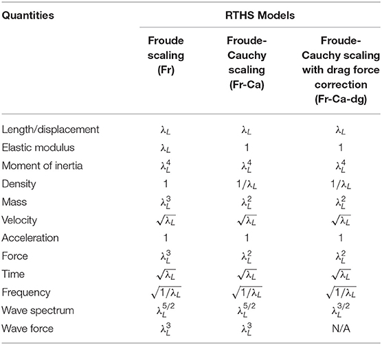
Table 2. Scaling relations for the RTHS models.

In all RTHS models, a length scale λ_L = 1/25 is used for the experimental component (the tower structure) and the water is considered as the fluid for the wave tank (hence λ_ρw = 1). Based on Table 2, it is noted that

i) The only scaling law completely preserves the similitude is the “Fr” model. The wave force generated in “Fr-Ca” and “Fr-Ca-dg” models does not match the force similitude of the tower structure. But it is noted that the specimen design is more challenging for the “Fr” model than the other two models as described in Section. Error contributors.

ii) The difference between “Fr-Ca” and “Fr-Ca-dg” models is that the wave spectrum is adjusted by a factor of 1/λ_L, or wave amplitude by a factor of $\sqrt{1/{\lambda }_L}$. As pointed out in Section. Error contributors, although such an adjustment preserves the similitude of drag force F_d, but the overall wave force scale is still distorted.

Study Cases

A total of five cases are considered in this study to evaluate the feasibility and identify error contributors of the proposed RTHS framework. In each case, sensitivity analysis is performed to determine the influence of the error contributors and their tolerances for a feasible RTHS design. The relative root-mean-square error (RMSE) between the responses obtained from RTHS and the prototype model is used to measure the performance. Prior to the RMSE calculation, the responses obtained from the RTHS models are scaled back to full-scale using the corresponding scale factors listed in Table 2. Each numerical simulation runs with a time step of 1/1,024 s and a duration of 120 s.

Case I: Delay

In this case, both the actuator delay and the sensor delay shown in Figure 7 are considered in the RTHS simulations. Seven different delayed time steps are considered, which are 0, 2, 3, 4, 6, 8, and 10, for both delays. Therefore, a total of 49 simulations are performed for each RTHS model. To focus on the impact from delay, noises are set as zero in all the simulations.

The RMSE for the responses u₇ and u₈ are summarized in Figure 8. The responses of these two DOFs are chosen because they are the interfacing DOFs whose accuracy directly impacts the accuracy of both numerical and experimental components, and hence the overall performance. Abbreviations “Fr,” “Fr-Ca,” and “Fr-Ca-dg” indicate RTHS models obtained using Froude scaling, Froude-Cauchy scaling, and Froude-Cauchy scaling with drag force correction, respectively. The axes “delay_A” and “delay_M” indicate the number of delayed time steps in actuator and sensor (measurement) systems, respectively.

FIGURE 8

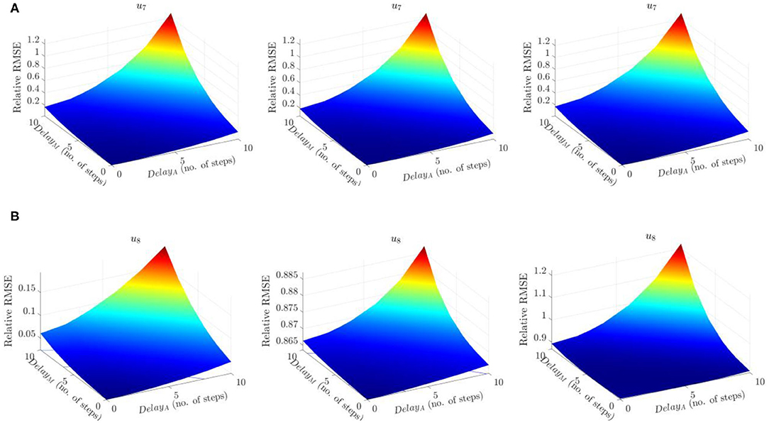
Figure 8. Case I: RMSE comparison. (A) RMSE of u₇, from left to right: Fr, Fr-Ca, Fr-Ca-dg. (B) RMSE of u₈, from left to right: Fr, Fr-Ca, Fr-Ca-dg.

From Figure 8, the RMSE error quickly increases as the delays increase. For the response in u₇ the performance of the three RTHS models are similar. But, for the response in u₈, the error in Fr model is much smaller than the other two, indicating a better performance due to its preserved similitude. The contrast between u₇ and u₈ is because most of the response in u₇ is induced by wind load, and most of the response in u₈ is induced by the hydrodynamic forces. The error in u₈ serves as a better indicator for scaling distortion in hydrodynamic force. For the RTHS models “Fr-Ca” and “Fr-Ca-dg,” where the hydrodynamic forces are distorted, their u₈ responses are expected with higher errors than the “Fr” model.

To determine the tolerance on delays, a closer view on the RMSE results indicates, when both delays are 3 steps, the RMSEs for the Fr, Fr-Ca, Fr-Ca-dg are 5.5, 9.3, 5.3% for u₇, and 3.4, 86.5, 87.0% for u₈. These results indicate that the drag force correction improves the accuracy of u₇ in the Fr-Ca-dg model comparing to the Fr-Ca model. But clearly, Fr model is the one that can provide accurate response estimation for both u₇ and u₈. When inspecting Figure 9, the time histories in the Fr-Ca-dg model indicates that, although the comparison between the “INTG” (prototype) and the “RTHS” in u₈ show obvious discrepancies, the amplitude of u₈ is much smaller (almost negligible) than u₇. Actually, the root-mean-square (RMS) value of u₈ is only 5% of that of u₇. Therefore, if only the significant fore-aft response is of concern, the Fr-Ca-dg RTHS model can also be considered as a viable alternative when both delays are 3 steps. For the Fr-Ca model, even when both delays are zero, the RMSE is still around 7%, which is the worst among all three RTHS models.

FIGURE 9

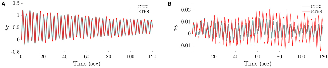
Figure 9. Case I: time history comparison in Fr-Ca-dg model (INTG—prototype; RTHS—RTHS model). (A) Time history of u₇. (B) Time history of u₈.

Case II: Noise

To determine the influence of noise on the performance of the proposed RTHS framework, both the actuator noise and the sensor noise shown in Figure 7 are considered in the RTHS simulations. The noises are generated as normally distributed random numbers with a zero mean and a standard deviation equal to a ratio of the standard deviation of the corresponding signal. r_A and r_M denote such ratios for the actuator noise and the sensor noise, respectively. Seven values for both ratios are chosen as 0, 1, 2, 5, 10, 15, and 20%. Therefore, a total of 49 simulations are performed for each RTHS model. To focus on the impact from noise, delays are set as zero in all the simulations.

From Figure 10, it is shown that, for u₇, both the Fr and the Fr-Ca-dg models produce smaller errors than the Fr-Ca model; for u₈, the Fr model yields the smallest error, and both the Fr-Ca and the Fr-Ca-dg models produce similar levels of error, due to their distorted hydrodynamic effects. The contour lines in parallel to r_M axis in all the graphs indicate that the RMSEs are more sensitive to the noise levels in the actuator system than in the sensor system. The reason is that the numerical component simulated in full-scale has lower natural frequencies than the experimental component. The sensor noises fed into the numerical system is effectively “filtered” by the numerical system and impose little influence on the system responses. While most of the RMSE results demonstrate an increasing trend with respect to the noise level, the RMSE of u₈ in the Fr-Ca-dg model shows a decreasing phase before the increasing trend. The exact reason to this observation is unknown, but it may be related to the drag force correction. The RMSEs of the blade responses (u₁~u₆) are also examined, but only small changes are shown with the considered noise range, and therefore are not shown in this study.

FIGURE 10

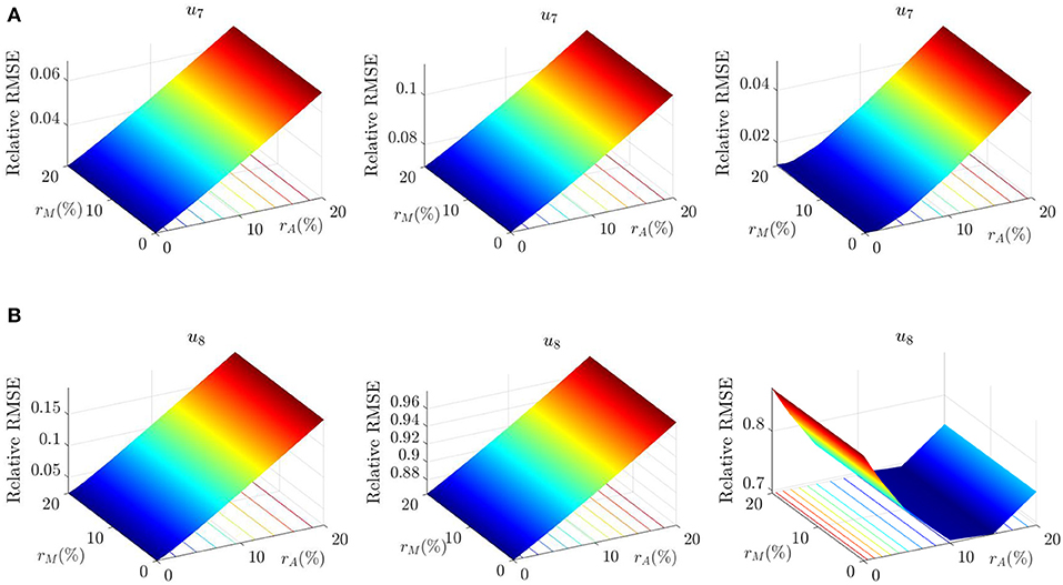
Figure 10. Case II: RMSE comparison. (A) RMSE of u₇, from left to right: Fr, Fr-Ca, Fr-Ca-dg. (B) RMSE of u₈, from left to right: Fr, Fr-Ca, Fr-Ca-dg.

Because the RMSEs show weak sensitivity with respect to the sensor noises, Table 3 is prepared by averaging all the RMSEs with the same actuator noise levels but different sensor noises.

TABLE 3

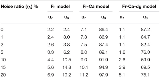
Table 3. Averaged RMSE (%) for Case II: actuator noise impact.

Based on Table 3, it can be seen that the Fr-Ca-dg model yields the smallest error on u₇, and the next is the Fr model. Both of them yield around 4 − 5% error under 15% level of noise. The Fr-Ca model, however, produces more than 10% RMSE at 15% level of noise. For u₈, similar as Case I, only the Fr model can produce accurate tracking up to 5% level of noise. Again, if u₈ is not of concern, then both the Fr and the Fr-Ca-dg models can be adopted for RTHS development.

Case III: Delay Combined With Noise

To examine the performance under combined effects of delay and noise, the actuator delay and the sensor delay are set to be equal to each other with the seven predetermined values, i.e., delay_A = delay_M = delay = 0, 2, 3, 4, 6, 8, and 10; and the noises are also set in a similar manner with r_A = r_M = r = 0, 1, 2, 5, 10, 15, and 20%. A total of 49 simulations are performed for each RTHS model.

In Figure 11, three RMSE plots are presented for the Fr model. The blade response u₁ is selected to represent the blade edgewise responses, u₁~u₃, and u₄ to represent the flapwise responses, u₄~u₆. All three plots indicate an increasing trend with response to the delays, and the contour lines show that RMSEs are more sensitive to the delays than to the noise levels. It is also noted that the blade flapwise response u₄ has a much higher RMSE value than the others, which is inspected further when discussing the tolerance. It is observed that the RMSEs of u₁, u₄, and u₇ in the Fr-Ca and Fr-Ca-dg models are similar as those in Figure 11, and therefore are not repeated here.

FIGURE 11

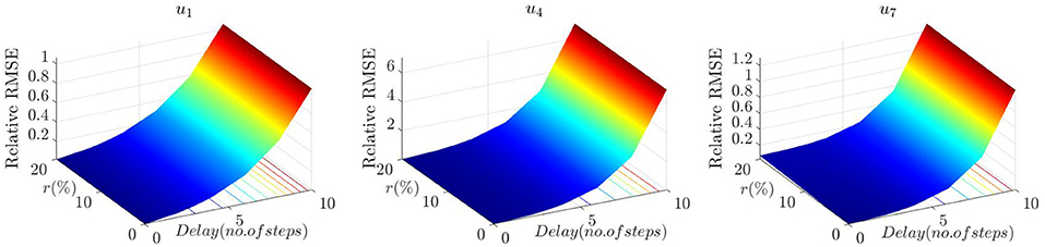
Figure 11. Case III: RMSE comparison for u₁, u₄, and u₇ in Fr model.

The RMSEs for u₈ of the three RTHS models are compared in Figure 12. They all show sensitivities to both delay and noise levels to some extent. The Fr-Ca model shows higher sensitivity to noises than to delays, while the Fr model shows similar levels of sensitivities to both. The Fr-Ca-dg model provides a non-monotonic relation against noise, which matches the observation made in Case II. The RMSEs in the Fr-Ca and Fr-Ca-dg models are much higher than the Fr model, similar as observed from Cases I and II.

FIGURE 12

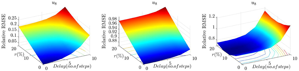
Figure 12. Case III: RMSE comparison for u₈ (from left to right: Fr, Fr-Ca, Fr-Ca-dg).

Because the RMSEs of u₁, u₄, and u₇ show weak sensitivity to noise levels, Table 4 is prepared to demonstrate the delay impacts on error tolerance by averaging all the RMSEs with the same delays but different noise levels. Note that the delays applied in this section carry a doubled-effect because both actuator and sensor are specified with the same amount of delay. Based on the results in Table 4, all three models show similar performance for u₁ and u₄. For u₇, both the Fr and Fr-Ca-dg models provide superior performance to the Fr-Ca model, and Fr-Ca-dg model is slightly better than the Fr model. It is noted that, even with very low delays, the RMSE for u₄ is around 4% and increases rapidly as the delay increases. However, such a level of RMSEs in the blade responses do not induce a large error in the tower response, u₇, because tower is evaluated under a reduced scale and the errors in the full-scale blade responses are reduced accordingly before sending to the experimental component. Therefore, if the blade responses are of interest, the RTHS implementation needs to guarantee a well-compensated RTHS to address the delay issues. To further understand the behavior of the scaled RTHS model, 20 s of time histories of the actuator force (in x direction), ${\text{F}}_{\text{I}}^{\text{N}}-{\text{f}}_{\text{I}}^{\text{E}}$, the sensor measurement (in x direction), ${\ddot{\text{u}}}_{\text{I}}$, and the responses, u₄ and u₇, are shown in Figure 13 for the Fr model with delay = 2 and r = 20%. In the plots, the “INTG” curve indicates the prototype behavior without delay and noise, and the “RTHS” curve indicates the behavior from the Fr model. It can be seen that although the actuator force and sensor measurement are contaminated by noises, the responses show fairly smooth behavior and follow the natural frequencies of the blade and the tower. The reason is the broadband noises are effectively filtered by the blade and tower which has low fundamental frequencies (see Table 1) even after the scaling.

TABLE 4

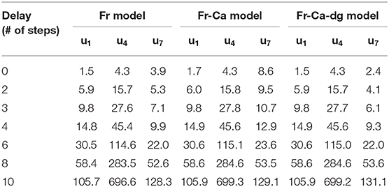
Table 4. Averaged RMSE (%) for Case III: delay impact.

FIGURE 13

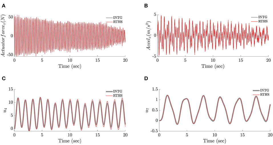
Figure 13. Case III: time history comparison in Fr model for delay = 2 and r = 20% (INTG—prototype; RTHS—RTHS model). (A) Time history of actuator force. (B) Time history of sensor measurement. (C) Time history of u₄. (D) Time history of u₇.

Case IV: Misalignment Angle

The misalignment angle β = 30° is applied in Cases I, II, and III. Based on their results, the errors generated in RTHS models are closely related to the delays and noise levels. For the Fr-Ca and Fr-Ca-dg models, the errors are also attributed to the distorted hydrodynamic effects. Therefore, the hydrodynamic load generation is further examined. In this case, the impact of misalignment angle β on the RTHS performance is studied. For each RTHS model, three nominal delay-noise combinations are considered:

• Good condition: delay_A = delay_M = delay = 1, r_A = r_M = r = 1%;

• Medium condition: delay_A = delay_M = delay = 3, r_A = r_M = r = 5%;

• Bad condition: delay_A = delay_M = delay = 6, r_A = r_M = r = 10%.

These conditions correspond to the quality of the actuator compensation design and fidelity of the sensor signals. For each condition, the misalignment angles ranging from 0° to 360° are considered with an increment of 15°.

The RMSE results for u₇ and u₈ are shown in Figure 14. For u₇, the performances of the Fr and the Fr-Ca-dg model are similar and show no particular dependence on β. The Fr-Ca model, however, shows that the errors near β = 90° or 270° are lower than the other β values. For u₈, only the Fr model demonstrates RMSE values lower than 5% in all β values under the good condition. The Fr model also shows that higher RMSEs are expected when β is near 0° or 180° in all conditions. In contrast, for the Fr-Ca and the Fr-Ca-dg models, the RMSE is lower (around 5%) when β is near 0° or 180° (alongwind) under the good condition. This observation is expected because the distorted hydrodynamic effects only influence the fore-aft responses in this case and causes a lower impact in the side-side responses comparing to the wind load. High RMSEs are expected in other β values. Therefore, they can be considered for RTHS implementation for the alongwind cases. The RMSEs of the blade responses (u₁~u₆) for all three RTHS models are also examined. They show no particular dependence on β, and therefore, are not repeated here.

FIGURE 14

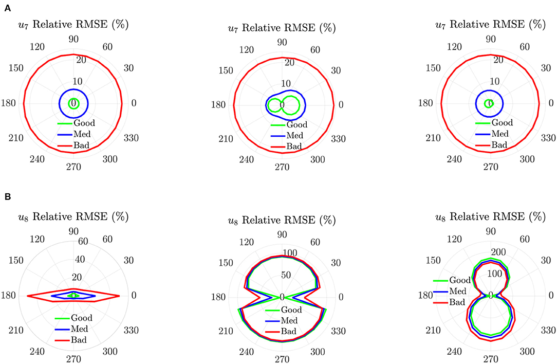
Figure 14. Case IV: RMSE comparison. (A) RMSE of u₇, from left to right: Fr, Fr-Ca, Fr-Ca-dg. (B) RMSE of u₈, from left to right: Fr, Fr-Ca, Fr-Ca-dg.

Case V: Wave Height

Another parameter related to the hydrodynamic load generation is the significant wave height H_s. In all previous cases, a significant wave height H_s = 3m is used. To study the impact of different wave heights on the RTHS performance, H_s values equal to 0.5, 1.5, 3, and 4.5 m, are considered. For each H_s value, the misalignment angles ranging from 0° to 360° are considered with an increment of 15°. In all simulations, only the “good condition” delay-noise combination is applied, i.e., delay_A = delay_M = delay = 1, r_A = r_M = r = 1%.

The RMSE results for u₇ and u₈ are shown in Figure 15. For u₇, the Fr model shows no particular dependence on H_s. The Fr-Ca-dg model provides similar RMSEs as the Fr model, except near the region β = 120° ~ 240°, where the error increases as H_s increases. The RMSEs in Fr-Ca-dg model increase as H_s increases, except near β = 90° or 270°, where the errors are lower and insensitive to the change in H_s. For u₈, only the Fr model provides RMSE values lower than 5% in all β values. The RMSE in the Fr model demonstrates a deceasing trend as H_s increases and reaches the highest values when β is near 0° or 180°. Both the Fr-Ca and the Fr-Ca-dg models show an RMSE increasing trend as H_s increases. In contrast to the Fr model, their RMSEs reaches the lowest values (around 5%) when β is near 0° or 180° (alongwind), and the highest when β is near 90° or 270° (crosswind). This observation is consistent with Case IV. The RMSEs of the blade responses (u₁~u₆) for all three RTHS models are also examined. They show no particular dependence on H_s, and therefore are not repeated here.

FIGURE 15

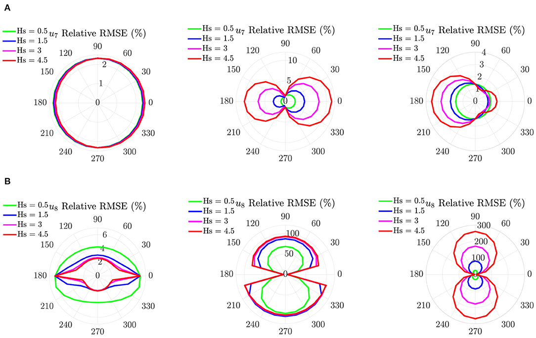
Figure 15. Case V: RMSE comparison. (A) RMSE of u₇, from left to right: Fr, Fr-Ca, Fr-Ca-dg. (B) RMSE of u₈, from left to right: Fr, Fr-Ca, Fr-Ca-dg.

Conclusions

In this study, a RTHS framework for monopile OWT is proposed. Three RTHS models, representing three different scaling laws, are modeled and simulated. By comparing their responses with those of the prototype in a set of sensitivity analyses, the performance and the possible error contributors of the proposed RTHS are evaluated. The findings provide important insights for future RTHS implementations. These findings include:

• RTHS using Froude scaling (the Fr RTHS) can provide the best overall performance in capturing the responses in both the numerical (blades) and the experiment (tower) components. It can achieve <5% RMSE for all responses with all misalignment angles and wave heights under the “good condition,” i.e., delay_A = delay_M = delay = 1, r_A = r_M = r = 1%. Its specimen design and construction are more challenging than the other two scaling laws considered. But if the difficulty in specimen design can be overcome, the Froude scaling RTHS is the preferred method for RTHS implementation.

• RTHS using Froude-Cauchy scaling with drag force correction (the Fr-Ca-dg RTHS) is a viable alternative to the one with Froude scaling. It offers similar performance as the Fr model in almost all responses, except the ones in side-side direction (u₈), due to the distorted hydrodynamic effects. However, if the responses in side-side direction is not of concern or when they are in much lower amplitude than the wind-induced responses, for example, when the wave is aligned with the wind direction (β is near 0° and 180°), the Fr-Ca-dg RTHS can also be considered for RTHS implementation. Its advantage over the Froude scaling is in the specimen design—it provides a systematic way to construct the scaled specimen (using added artificial mass).

• RTHS using the conventional Froude-Cauchy scaling (the Fr-Ca RTHS) is the least attractive one in this study. It offers the same advantage in specimen design and construction like the Fr-Ca-dg model, and it has the same issue on capturing the side-side responses. But even for the fore-aft response (e.g., u₇), it demonstrates lower robustness against noise and delay comparing to the Fr-Ca-dg RTHS (see Tables 3, 4). It does have an advantage over the Fr-Ca-dg RTHS in that it is less demanding in the wave generation, as it does not require the drag force correction.

• Even with the Froude scaling, it is observed that, the proposed RTHS framework is more sensitive to the delays than to the noises, and it is more sensitive to the actuator noises than to the sensor noises.

• To accurately capture the responses in blades, a small (around 1~2 steps) delay needs to be specified. If only the responses in tower is of concern, the delay requirement can be relaxed to 4~6 steps (see Table 4).

As a concept study, only numerical simulations are considered herein, and the modeling parameters are selected to represent typical OWT behavior to investigate the proposed RTHS framework. Experimental implementations of the proposed RTHS framework will be carried out in the future. In addition, torsional DOFs of the tower are not considered at the current stage. As the study further develops, more complex modeling techniques, and loading cases will be considered in implementing the proposed RTHS framework with specific OWT designs and site conditions.

Data Availability Statement

The datasets generated for this study are available on request to the corresponding author.

Author Contributions

WS completed the main writing task of the paper and the main coding. Oversee the development of the study presented in the paper. CS completed part of the coding (on wave load generation) used in the analysis. YZ completed part of the literature review and the writing of the paper. VJ completed part of the coding (on wind load generation) used in the analysis. YL contribute to the review, editing, and assist the development of the study presented in the paper. QH contribute to the review, editing, and assist the development of the study presented in the paper. All authors contributed to the article and approved the submitted version.

Conflict of Interest

The authors declare that the research was conducted in the absence of any commercial or financial relationships that could be construed as a potential conflict of interest.

Supplementary Material

The Supplementary Material for this article can be found online at: https://www.frontiersin.org/articles/10.3389/fbuil.2020.00129/full#supplementary-material

References

Aasen, S., Page, A., Skau, K., and Nygaard, T. (2017). Effect of foundation modelling on the fatigue lifetime of a monopile-based offshore wind turbine. Wind Energy Sci. 2, 361–376. doi: 10.5194/wes-2-361-2017

CrossRef Full Text | Google Scholar

Abbiati, G., Marelli, S., Tsokanas, N., Sudret, B., and Stojadinović, B. (2021). A global sensitivity analysis framework for hybrid simulation. Mech. Syst. Signal Process. 146:106997. doi: 10.1016/j.ymssp.2020.106997

CrossRef Full Text | Google Scholar

Alagan Chella, M., Tørum, A., and Myrhaug, D. (2012). An overview of wave impact forces on offshore wind turbine substructures. Energy Procedia 20, 217–226. doi: 10.1016/j.egypro.2012.03.022

CrossRef Full Text | Google Scholar

Anaya-Lara, O., Tande, J. O., Uhlen, K., and Merz, K. (2018). Offshore Wind Energy Technology. Hoboken, NJ: Wiley Online Library.

Google Scholar

Arany, L., Bhattacharya, S., Macdonald, J., and Hogan, S. J. (2017). Design of monopiles for offshore wind turbines in 10 steps. Soil Dyn. Earthq. Eng. 92, 126–152. doi: 10.1016/j.soildyn.2016.09.024

CrossRef Full Text | Google Scholar

Barj, L., Jonkman, J. M., Robertson, A., Stewart, G. M., Lackner, M. A., Haid, L., et al. (2014). “Wind/wave misalignment in the loads analysis of a floating offshore wind turbine,” in 32nd ASME Wind Energy Symposium (National Harbor, MD: American Institute of Aeronautics and Astronautics).

Google Scholar

Bhattacharya, S. (2019). Design of Foundations for Offshore Wind Turbines. Hoboken, NJ: Wiley Online Library.

Google Scholar

Bredmose, H., Larsen, S., Matha, D., Rettenmeier, A., Marino, E., and Saettran, L. (2012). Marine Renewables Infrastructure Network (MARINET) Report. Collation of offshore wind wave dynamics.

Campagnolo, F. (2013). Wind Tunnel Testing of Scaled Wind Turbine Models: Aerodynamics and Beyond. Milan: Politecnico di Milano.

Google Scholar

Canet, H., Bortolotti, P., and Bottasso, C. L. (2018). Gravo-aeroelastic scaling of very large wind turbines to wind tunnel size. J. Phys. Conf. Ser. 1037:042006. doi: 10.1088/1742-6596/1037/4/042006

CrossRef Full Text | Google Scholar

Carrion, J. E., and Spencer, B. F. Jr. (2007). Model-based Strategies for Real-time Hybrid Testing. Newmark Structural Engineering Laboratory Report Series 006, Urbana, IL: University of Illinois at Urbana-Champaign.

Google Scholar

Carswell, W., Johansson, J., Løvholt, F., Arwade, S. R., Madshus, C., Degroot, D. J., et al. (2015). Foundation damping and the dynamics of offshore wind turbine monopiles. Renew. Energy 80, 724–736. doi: 10.1016/j.renene.2015.02.058

CrossRef Full Text | Google Scholar

Chabaud, V., Steen, S., and Skjetne, R. (2013). “Real-time hybrid testing for marine structures: challenges and strategies,” in 2013 32nd International Conference on Ocean, Offshore and Arctic Engineering (Nantes: ASME).

Google Scholar

Christenson, R., Dyke, S. J., Zhang, J., Mosqueda, G., Chen, C., Nakata, N., et al. (2014). “Hybrid simulation: a discussion of current assessment measures,” in Hybrid Simulation Task Force Meeting sponsored by US National Science Foundation (NSF) (West Lafayette, IN).

Craig, R. R., and Kurdila, A. J. (2006). Fundamentals of Structural Dynamics, 2^nd Ed. John Wiley & Sons.

Google Scholar

De Ridder, E.-J., Otto, W., Zondervan, G.-J., Huijs, F., and Vaz, G. (2014). “Development of a scaled-down floating wind turbine for offshore basin testing,” in 2014 33rd International Conference on Ocean, Offshore and Arctic Engineering (San Francisco, CA: American Society of Mechanical Engineers Digital Collection).

Google Scholar

Dnvgl. (2010). DNVGL-RP-C205 Environmental Conditions and Environmental Loads. DNVGL.

Dnvgl. (2016). DNVGL-ST-0126 Support Structures for Wind Turbines. Olso: DNV GL.

Du, W., Zhao, Y., He, Y., and Liu, Y. (2016). Design, analysis and test of a model turbine blade for a wave basin test of floating wind turbines. Renew. Energy 97, 414–421. doi: 10.1016/j.renene.2016.06.008

CrossRef Full Text | Google Scholar

Esteban, M. D., Diez, J. J., López, J. S., and Negro, V. (2011). Why offshore wind energy? Renew. Energy 36, 444–450. doi: 10.1016/j.renene.2010.07.009

CrossRef Full Text | Google Scholar

Faltinsen, O. (1990). Sea Loads on Ships and Offshore Structures. Cambridge, UK: Cambridge University Press.

Google Scholar

Hall, M., Goupee, A., and Jonkman, J. (2018). Development of performance specifications for hybrid modeling of floating wind turbines in wave basin tests. J. Ocean Eng. Mar. Energy 4, 1–23. doi: 10.1007/s40722-017-0089-3

CrossRef Full Text | Google Scholar

Hall, M., Moreno, J., and Thiagarajan, K. (2014). “Performance specifications for real-time hybrid testing of 1:50-scale floating wind turbine models,” in International Conference on Offshore Mechanics and Arctic Engineering (San Francisco, CA: American Society of Mechanical Engineers).

Google Scholar

Hansen, M. O. (2015). Aerodynamics of Wind Turbines 3rd Ed. London; New York, NY: Routledge.

Google Scholar

Hasselmann, K., Barnett, T., Bouws, E., Carlson, H., Cartwright, D., Enke, K., et al. (1973). Measurements of wind-wave growth and swell decay during the Joint North Sea wave project (JONSWAP). Deut. Hydrogr. Z 8, 1–95.

Google Scholar

Hayati, S., and Song, W. (2017). An optimal discrete-time feedforward compensator for real-time hybrid simulation. Smart Struct. Syst. 20, 483–498. doi: 10.1007/978-3-319-54777-0_27

CrossRef Full Text | Google Scholar

Hayati, S., and Song, W. (2018). Design and Performance Evaluation of an Optimal Discrete-Time Feedforward Controller for Servo-Hydraulic Compensation. J. Eng. Mech. 144:04017163. doi: 10.1061/(ASCE)EM.1943-7889.0001399

CrossRef Full Text | Google Scholar

Iec. (2005). IEC 61400-1 Wind Turbines Part 1: Design Requirements. International Electrotechnical Commission.

Google Scholar

Jonkman, B. J., and Kilcher, L. (2012). Turbsim User's Guide: Version 1.06.00. Golden, CO: National Renewable Energy Lab (NREL), 87.

Jonkman, J., Butterfield, S., Musial, W., and Scott, G. (2009). Definition of a 5-MW Reference Wind Turbine for Offshore System Development. Golden, CO: National Renewable Energy Laboratory.

Google Scholar

Keivanpour, S., Ramudhin, A., and Ait Kadi, D. (2017). The sustainable worldwide offshore wind energy potential: a systematic review. J. Renew. Sustain. Energy 9:065902. doi: 10.1063/1.5009948

CrossRef Full Text | Google Scholar

Kimball, R., Goupee, A. J., Fowler, M. J., De Ridder, E.-J., and Helder, J. (2014). “Wind/wave basin verification of a performance-matched scale-model wind turbine on a floating offshore wind turbine platform,” in International Conference on Offshore Mechanics and Arctic Engineering ( San Francisco, CA: American Society of Mechanical Engineers).

Google Scholar

Lamb, H. (1945). Hydrodynamics, 6th Revised Ed. New York, NY: Dover Publications.

Maghareh, A., Dyke, S. J., Prakash, A., and Bunting, G. B. (2014). Establishing a predictive performance indicator for real-time hybrid simulation. Earthq. Eng. Struct. Dyn. 43, 2299–2318. doi: 10.1002/eqe.2448

CrossRef Full Text | Google Scholar

Martin, H. R. (2011). Development of a Scale Model Wind Turbine for Testing of Offshore Floating Wind Turbine Systems. MS Thesis, Orono, ME: The University of Maine.

Google Scholar

Martin, H. R., Kimball, R. W., Viselli, A. M., and Goupee, A. J. (2014). Methodology for wind/wave basin testing of floating offshore wind turbines. J. Offshore Mech. Arctic Eng. 136:020905. doi: 10.1115/1.4025030

CrossRef Full Text | Google Scholar

MathWorks (2020). MATLAB R2020a. Natick, MA.

Morató, A., Sriramula, S., Krishnan, N., and Nichols, J. (2017). Ultimate loads and response analysis of a monopile supported offshore wind turbine using fully coupled simulation. Renew. Energy 101, 126–143. doi: 10.1016/j.renene.2016.08.056

CrossRef Full Text | Google Scholar

Morison, J., O'brien, M., Johnson, J., and Schaaf, S. (1950). The force exerted by surface waves on piles. Petroleum Trans. 189, 149–154. doi: 10.2118/950149-G

CrossRef Full Text

Musial, W., Heimiller, D., Beiter, P., Scott, G., and Draxl, C. (2016). 2016 Offshore Wind Energy Resource Assessment for the United States. Golden, MO: National Renewable Energy Lab (NREL).

Google Scholar

Nakashima, M., Kato, H., and Takaoka, E. (1992). Development of real-time pseudo dynamic testing. Earthq. Eng. Struct. Dyn. 21, 79–92. doi: 10.1002/eqe.4290210106

CrossRef Full Text | Google Scholar

Newman, J. N. (1977). Marine Hydrodynamics. Cambridge, MA: The MIT Press.

Google Scholar

Perveen, R., Kishor, N., and Mohanty, S. R. (2014). Off-shore wind farm development: present status and challenges. Renew. Sustain. Energy Rev. 29, 780–792. doi: 10.1016/j.rser.2013.08.108

CrossRef Full Text | Google Scholar

Phillips, B. M., and Spencer, B. F. Jr. (2012). Model-Based Framework for Real-Time Dynamic Structural Performance Evaluation. Newmark Structural Engineering Laboratory Report Series 031, Urbana, IL: University of Illinois at Urbana-Champaign.

Google Scholar

Pierson, W. J. Jr., and Moskowitz, L. (1964). A proposed spectral form for fully developed wind seas based on the similarity theory of S. A. Kitaigorodskii. J. Geophys. Res. 69, 5181–5190. doi: 10.1029/JZ069i024p05181

CrossRef Full Text | Google Scholar

Przemieniecki, J. S. (1968). Theory of Matrix Structural Analysis. New York, NY: McGraw-Hill.

Google Scholar

Robertson, A., Jonkman, J., Goupee, A., Coulling, A., Prowell, I., Browning, J., et al. (2013). “Summary of conclusions and recommendations drawn from the deepcwind scaled floating offshore wind system test campaign,” in International Conference on Offshore Mechanics and Arctic Engineering (Nante: sAmerican Society of Mechanical Engineers).

Google Scholar

Sauder, T., Chabaud, V., Thys, M., Bachynski, E. E., and Sæther, L. O. (2016). “Real-time hybrid model testing of a braceless semi-submersible wind turbine: part I—the hybrid approach,” in 2016 35th International Conference on Ocean, Offshore and Arctic Engineering (Busan: ASME).

Google Scholar

Sauder, T., Marelli, S., and Sørensen, A. J. (2019). Probabilistic robust design of control systems for high-fidelity cyber–physical testing. Automatica 101, 111–119. doi: 10.1016/j.automatica.2018.11.040

CrossRef Full Text | Google Scholar

Stansby, P. K., Devaney, L., and Stallard, T. (2013). Breaking wave loads on monopiles for offshore wind turbines and estimation of extreme overturning moment. Renew. Power Gener. 7, 514–520. doi: 10.1049/iet-rpg.2012.0205

CrossRef Full Text | Google Scholar

Sun, C. (2018a). Mitigation of offshore wind turbine responses under wind and wave loading: Considering soil effects and damage. Struct. Control. Health Monit. 25:e2117. doi: 10.1002/stc.2117

CrossRef Full Text | Google Scholar

Sun, C. (2018b). Semi-active control of monopile offshore wind turbines under multi-hazards. Mech. Syst. Signal Process. 99, 285–305. doi: 10.1016/j.ymssp.2017.06.016

CrossRef Full Text | Google Scholar

Sun, C., and Jahangiri, V. (2018). Bi-directional vibration control of offshore wind turbines using a 3D pendulum tuned mass damper. Mech. Syst. Signal Process. 105, 338–360. doi: 10.1016/j.ymssp.2017.12.011

CrossRef Full Text | Google Scholar

Thys, M., Chabaud, V., Sauder, T., Eliassen, L., Sæther, L. O., and Magnussen, Ø. B. (2018). “Real-time hybrid model testing of a semi-submersible 10MW floating wind turbine and advances in the test method,” in 2018 1st International Offshore Wind Technical Conference (San Francisco, CA: ASME).

Google Scholar

Wu, T., and Song, W. (2019). Real-time aerodynamics hybrid simulation: wind-induced effects on a reduced-scale building equipped with full-scale dampers. J. Wind Eng. Ind. Aerod. 190, 1–9. doi: 10.1016/j.jweia.2019.04.005

CrossRef Full Text | Google Scholar