An Integrated Microclimate-Energy Demand Simulation Method for the Assessment of Urban Districts

Introduction

In proceeding through the “Grand Transition”, global energy consumption is predicted to increase by 22 to 46% by 2060 (World Energy Council, 2016). A large part of this increase is due to worldwide demographic growth in urbanized areas. European cities have also seen a faster overall rise in number of inhabitants in the last decade (Eurostat, 2016). This trend, combined with an urbanization shift from an expansive development model to a compact and concentrated one, has resulted in redevelopment projects in inner-city areas. Urban re-densification processes as well as new urban developments need to meet design objectives of sustainability and livability generating new positive impacts on the surrounding urban environment. In order to achieve these, they need to comply with several climate and energy targets that aim to reduce greenhouse gas emissions, increase energy efficiency, and mitigate climate impacts such as heat stress.

One of the main challenges during the urban design process is predicting the effect of the urban form on the local microclimate, which influences not only outdoor thermal comfort but also the energy performance of buildings. Previous empirical and fundamental studies have shown that it is of growing importance to take the local climatic conditions into account when analyzing building energy performance and its environmental impact (Magli et al., 2015; Skelhorn et al., 2016). Anthropogenic heat, urban geometry and construction materials influence local thermal and wind patterns, thus affecting the climate context in which the buildings are operated (Santamouris et al., 2001). Phenomena of urban overheating such as the Urban Heat Island (UHI) have been shown to significantly increase space cooling demand (Hirano and Fujita, 2012; Liu et al., 2017; Guattari et al., 2018) and reduce heating consumption (Cui et al., 2017; Sun and Augenbroe, 2014) in different geographical zones. According to Li et al. (2019), UHI could result in an average increase in the electricity demand for cooling of 19% with intercity variations ranging between 10% and 120%. Moreover, as shown by the comparative analysis of Santamouris (2014) the peak electricity demand for cooling increases by 0.45 to 4.6% per degree increase in ambient temperature.

Despite the advancement of microclimate models and the growing need for more accurate energy assessment, computational models commonly used to support the understanding of building energy performance largely overlook urban microclimate phenomena. Meteorological boundary conditions adopted in Building Energy Simulations (BES) are typically based on Typical Meteorological Year (TMY) data from weather stations, which are usually smoothed and averaged over several years (Yang et al., 2012) and ignore the effect of the urban surroundings on local climate (Gobakis and Kolokotsa, 2017). As a consequence, energy assessments usually neglect the effects of urban overheating on base and peak energy demands, potentially compromising the decisions on energy strategies for future sustainable and low carbon districts.

This study aims to establish an integrated simulation method by coupling a state-of-the-art district-scale energy demand model with a microclimate simulation tool to quantitatively evaluate the effects of local climate on the energy consumption and peak power demand of individual buildings during extreme weather events. By expanding the scale from single buildings to the district level, the proposed method enables the analysis of the reciprocal influence between groups of buildings with different form, materials and orientation. The selected simulation tools are the microclimate software ENVI-met (Bruse and Fleer, 2009), which simulates small scale outdoor conditions, and the City Energy Analyst (CEA) (The CEA Team, 2018), an open-source tool for district-scale energy demand modeling and supply system optimization.

The first section of this paper provides a background on the effects of urban microclimate on energy demand and presents the state of the art in microclimate and energy demand modeling. The following section describes the simulation tools used in this paper and the coupling method, which involves extracting hourly based output data for air temperature, wind speed and relative humidity from the microclimate simulation and passing them to the energy demand simulation as the climatic boundary conditions. The method is then applied to analyze the energy performance of a case study in central Zurich (Switzerland). In order to demonstrate the approach, two consecutive hot days with clear sky were selected during the heat wave that affected Zurich in 2015. The results of simulations carried out with general weather data and with urban microclimatic data are subsequently compared, showing the effect on space cooling demand and peak cooling power in the district. Finally, conclusions are presented regarding limitations of the method, possibilities for its improvement, as well as for its use in urban design.

Background and State of the Art

Several physical phenomena that take place in the urban environment influence the thermal exchange processes of buildings. First, multiple interreflections of radiation and decreased sky view due to urban geometry, limited evapotranspiration due to sealed surfaces and scarce vegetation, and the thermal properties of construction materials used in buildings and paved areas, along with anthropogenic heat sources, lead to temperature differences between urban and rural areas. This phenomenon, known as the Urban Heat Island (UHI) effect, results in a reduction in heating demand and an increase in cooling demand in dense urban contexts (Allegrini et al., 2012). A second type of effect concerns wind patterns occurring within the canopy layer. In general, average wind speeds are lower in the urban environment (Allegrini et al., 2015); however, street network characteristics, building geometry and orientation, and the topographic location can cause significant local differences in speed as well as direction (Oke et al., 2017). These in turn affect the potential for natural ventilation and passive cooling. For example, the acceleration of air flows along street canyons increases thermal losses from building façades due to convective heat transfer, increasing heating demand during cold seasons. A third phenomenon is related to the influence of shortwave and longwave solar radiation. The compactness of the surrounding urban environment affects buildings’ exposure to solar radiation, both direct and reflected, leading to differences in thermal gains and the electricity demand for lighting (Allegrini et al., 2015).

Several simulation tools have been developed to model the urban climate. The main advantage of simulations compared to using measured weather station data is that they can generate explicit information for distinct climatic parameters (Toparlar et al., 2017). Prognostic Computational Fluid Dynamics models, in particular, allow the comparison of urban areas in the design stage under numerous time and climatic frames (Blocken, 2014; Mirzaei and Haghighat, 2010). Microclimate models predict detailed spatial distributions of flow, temperatures and scalar fields at the building to district scale (Ooka, 2007). Microclimate models take into account shortwave and longwave radiation, transpiration, evaporation and sensible heat fluxes, as well as heat exchange with the soil and can be of great use to assess the energy use in city districts (Sola et al., 2018).

Although microclimate has been recognized as a relevant factor in shaping energy consumption, computational models to predict building energy performance during the design process largely overlook urban microclimate phenomena. Allegrini et al. (2015) offered a comprehensive review of existing modeling approaches and tools which address the district scale of energy systems, and argued that “it is no longer sufficient to simulate building energy use assuming isolation from the microclimate and the energy system in which they operate”. Furthermore, the authors concluded that more extensive research is required into the link between thermal processes and microclimate effects, in terms of spatial and temporal detail, resolution and magnitude.

Recent advancements in computational approaches have allowed attempts to bridge this gap by coupling methods that link urban climatic variables to the thermal performance of buildings. A series of studies have presented coupling procedures between BEM and CFD in order to investigate the influence of urban climate on energy demand (Sánchez de la Flor and Álvarez Domínguez, 2004; He et al., 2008; Kolokotroni et al., 2010; Gros et al., 2016), to assess the influence of geometry and materials on urban temperatures and energy consumption (Gros et al., 2014; Toparlar et al., 2018), or to compare the performance of design measures to decrease heating and cooling loads (Skelhorn et al., 2016). However, previous work in this field has so far focused mainly on single buildings (e.g., Gobakis and Kolokotsa, 2017) and explorations of generic typologies employing homogeneous urban patterns that are not representative of the complexity of cities (e.g., He et al., 2008; Yang et al., 2012; Liu et al., 2015). On the other hand, attempts to couple district-scale energy demand simulations to urban climate models usually rely on simplified geometries and lower resolution mesoscale models (e.g., Rasheed et al., 2011; Mauree et al., 2016).

Planning energy systems at the district scale requires a detailed characterization of the energy needs of urban areas. In order to accurately account for the distribution of cooling loads in a district, it is necessary to explicitly simulate each building and their surrounding urban climate at the micro scale. However, the coupling at such a scale has as of yet not been carried out (Frayssinet et al., 2018). The main reason can be found in computational limitations, since the analysis of a large area such as a district in some cases surpasses the capability of energy simulation tools developed for single buildings, whereas urban building energy models (UBEM) have only been introduced relatively recently (Reinhart and Cerezo Davila, 2016).

Methodology

The proposed coupling approach, shown schematically in Figure 1, is based on passing simulated microclimate data from ENVI-met to the City Energy Analyst (CEA) to act as boundary conditions for building energy simulation. ENVI-met is a three-dimensional prognostic model designed to simulate heat, evapotranspiration and air flow processes between buildings, surfaces, and plants in urban environments, while CEA is an open-source tool for the analysis and optimization of energy systems in neighborhoods and city districts. The aim of the coupling method is to model the energy demand of a number of buildings at the district scale taking into account the various factors that influence energy performance, namely the microclimatic environment, locus and topographic context, and the building geometry and materials.

FIGURE 1

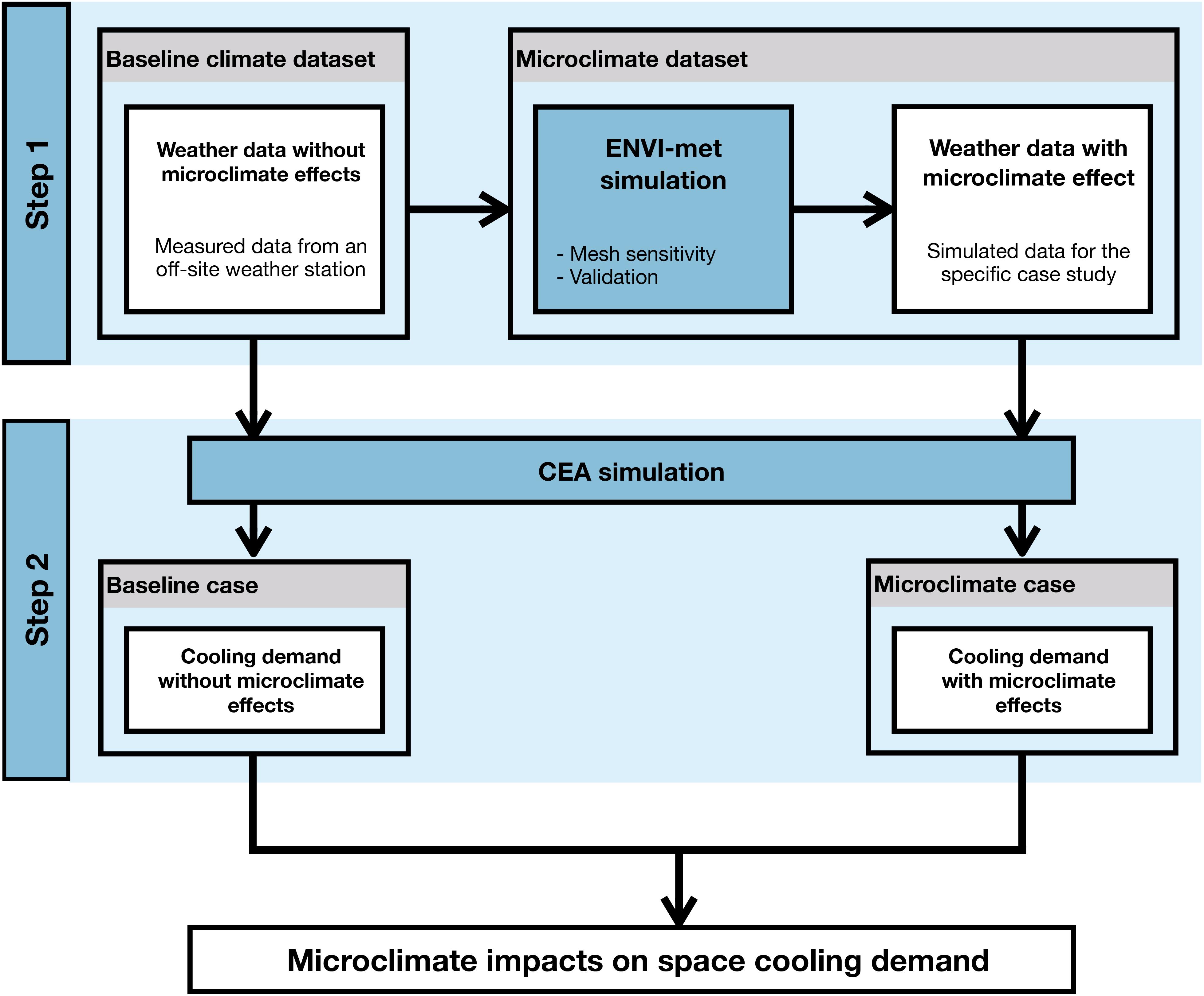
Figure 1. Schematic showing the proposed integration method between ENVI-met and CEA for each of the climatic cases considered.

In order to compare the effects of local microclimate on the predicted energy demands of the area, two climate datasets are prepared. The first consists of measured data from an offsite weather station, used as an input to the ENVI-met simulations as well as to CEA, where it provides a Baseline case. The second dataset, derived from ENVI-met simulations, reports the specific microclimate conditions within the area and is used to run a second energy demand simulation in the Microclimate case.

In the first step, the Baseline climate dataset for the offsite weather station is derived for a selected day. The model for the selected case study is built in ENVI-met 4.4 and validated against temperature data measured on location. The simulation results from ENVI-met for air temperature, wind speed and relative humidity for each façade are then averaged to obtain hourly values for each building in the area. Finally, the microclimate simulation results are passed to the City Energy Analyst (CEA) in order to carry out energy demand simulations. The software includes a dynamic model for building energy performance simulation, as well as tools for the assessment of local energy potentials, conversion and storage technology simulation, and energy system optimization.

The method presented here was developed and tested in a district in Zurich. For the application two consecutive hot days with clear sky were selected during the heat wave that affected Zurich in 2015. A detailed description of the case study and simulation settings are reported in section “Case Study Description.”

Step 1: Microclimate Modeling in ENVI-met

ENVI-met is a three-dimensional prognostic microclimate model designed to simulate the interaction between surfaces, plants and air in an urban environment (Bruse and Fleer, 2009). ENVI-met relies on Reynolds-Averaged Navier–Stokes equations to resolve heat transfer and fluid flows in urban settings. This approach reduces computational cost of the Computational Fluid Dynamics (CFD) model compared to large eddy simulation while achieving reasonable accuracy (Mirzaei and Haghighat, 2010). Moreover, ENVI-met has a typical resolution of 0.5 to 10 meters in space and a typical time frame of 24 to 48 h with a time step of 1 to 5 s. It consists of four models: an atmospheric model, a soil model, a vegetation model and a building model. The structure and equations that govern these sub-models are described in detail by Huttner (2012). The atmospheric model computes mean air flow, turbulence, fluxes of direct, diffuse and reflected short-wave and long-wave radiation, and air temperature and humidity. The soil model computes surface and soil temperatures and soil water fluxes and is coupled with the vegetation model, which calculates evaporation rates, foliage temperatures and exchanges of vegetation with the environment (heat, evaporation and transpiration fluxes). The building model computes fluxes of momentum, heat and vapor at and inside building walls and roofs taking into account material properties. The tool is well established to estimate and assess outdoor thermal comfort (Ali-Toudert and Mayer, 2006, 2007; Taleghani et al., 2015). In fewer cases it has also been used to estimate the impact of the urban microclimate on building energy demand, as is done in this study. Such studies have, however, only looked at the energy demand of single buildings, either theoretical typologies (Yang et al., 2012; Carnielo and Zinzi, 2013; Skelhorn et al., 2016) or existing case studies (Gobakis and Kolokotsa, 2017).

To perform an ENVI-met simulation, model input parameters must be provided for the Area Input file, Database, and Configuration file. The Area Input file (.INX) stores data regarding size and resolution of the domain, as well as spatial characteristics of the calculation mesh, by using an orthogonal 3D grid (either equidistant or telescoping), whose sizes in the x-, y- and z-directions can be defined by the user. Links with the Database ensure that descriptive parameters (such as thermal conductivity, albedo, water content, etc.) for soil, vegetation and surface materials can be used to solve equations of the mathematical model. Finally, the Configuration file (.SIMX) stores the simulation settings including weather boundary conditions. For the selected case study, section “Microclimate Dataset: Envi-met Model Construction and Parameters” describes data sources and input settings for the mentioned ENVI-met modules.

On the simulated results a mesh sensitivity analysis is performed and a validation procedure against measured temperature data is carried out. The validated model with the highest level of accuracy is selected for coupling with the energy model. The ENVI-met results consist of hourly values of a variety of climate parameters reported in a three-dimensional grid that can be exported in different formats. Atmospheric outputs report the values of various climate parameters, including: wind speed and direction; air temperature; mean radiant temperature; specific and relative humidity; turbulence kinetic energy; dissipation; vertical exchange coefficient; diffuse/reflected solar radiation; temperature and vapor flux; and CO₂ concentration. Given the simplified nature of the energy demand model used in CEA, only a few of these parameters are relevant for the energy demand simulation, namely air temperature, relative humidity, and wind speed. In the next section, the use of these values in CEA is described. Version 4.4 of ENVI-met allows users to export climate hourly results for each building. These are used in order to generate building-scale average hourly values of these climatic parameters, which are then passed as weather boundary conditions to CEA.

Step 2: Energy Demand Modeling in CEA and Main Environmental Parameters

The CEA thermal load model comprises two main sub-models, one for sensible loads and one for latent loads. The main environmental parameters that affect this model are the solar irradiation, relative humidity, outdoor temperature, and wind speed. The CEA urban solar radiation model is used to calculate the incident solar radiation in buildings accounting for both vertical and horizontal surfaces, material properties, shading, terrain topography and reflections. The tool first creates 3D representations of the geometry of buildings out of meta information about the size of windows, height, and number of floors in buildings. Each surface in the 3D representation is subdivided in a grid, and the calculation is performed at the centroid of every subdivision for every hour of the year. The calculation engine is based on the open source software DAYSIM (Reinhart, 2013), a validated radiation model for daylighting analysis. While fine-grained solar irradiation results for individual building surfaces can be obtained from DAYSIM, hourly values of air temperature, wind speed and relative humidity are usually obtained from weather stations in the form of Typical Meteorological Year data, which may not be representative of a district’s local climate. Therefore, these three parameters were selected for the study of the microclimate effects on space cooling demand.

Outdoor Air Temperature and Sensible Loads

The sensible load calculation implemented in CEA is based on a simplified resistance-capacitance model as described in Swiss norm (SIA Merkblatt 2044), which itself is an adaptation of ISO 13790 (2008). Each building in the area is represented by a single thermal zone, meaning that the building interior is assumed to be well-mixed with no effects from occupant distribution within the building or localized temperature differences.

The building material properties, solar gains, and internal gains caused by occupants as well as the use of lighting and appliances are then represented as resistances and capacitances in an electrical circuit, as shown in Figure 2. This system is composed of four nodes representing outdoor air, indoor air, a surface node, and a node in the building’s thermal mass. These nodes are connected by resistances representing building materials and systems, whose heat transfer coefficients are shown and described in the figure. The solar gains and the internal gains, which arise from building occupants and lighting and appliances in the building, are distributed among the three indoor nodes. The building also has an effective mass area and an internal heat capacity, which represents the thermal inertia in the building thermal mass. The derivation of these parameters is beyond the scope of this paper and can be found in the aforementioned standards. The goal of this model is to calculate, given the boundary conditions provided by the physical properties of the building and outdoor weather conditions, the heating or cooling required (Φ_HC) in order to satisfy the building’s set point temperature.

FIGURE 2

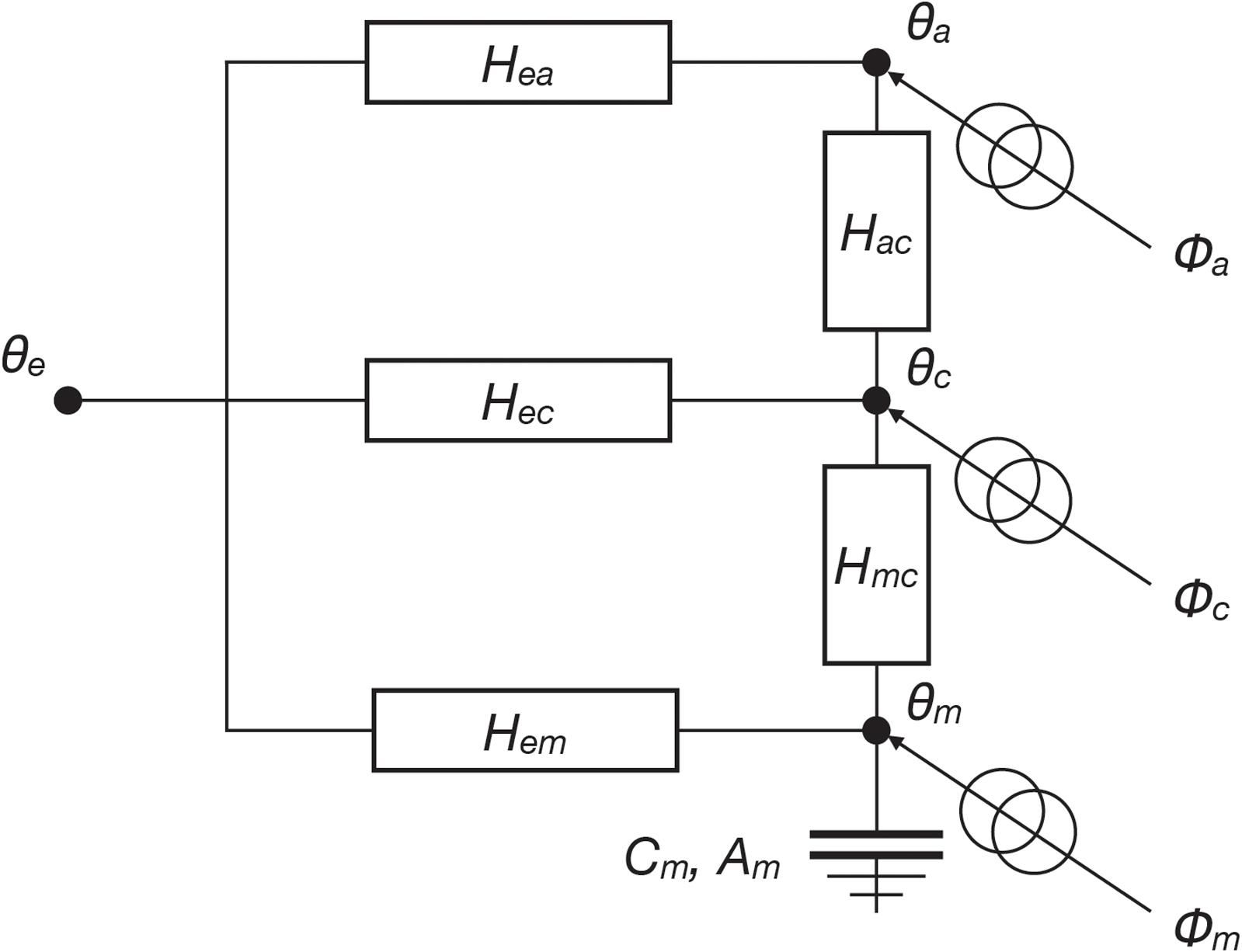
Figure 2. Resistance-capacitance (RC) model used in CEA (adapted from SIA Merkblatt 2044). θ_e, θ_a, θ_c, and θ_m are the temperatures of the exterior air, indoor air, surface node, and building thermal mass, respectively. H_ea is the air heat flow coefficient of the ventilation systems, whereas H_ec and H_em are the transmission heat coefficients lightweight and heavyweight building materials, respectively, and the heat transfer coefficients between the air and surface node, and between the surface node and the thermal mass are H_ac and H_mc, respectively. The internal and solar gains in the air, surface and thermal mass nodes are Φ_a, Φ_c and Φ_m, respectively. Finally, C_m and A_m are the internal heat capacity and effective mass area of the building.

Latent Load Calculation and Relative Humidity

In addition to these sensible loads, buildings with mechanical ventilation systems and air-based cooling systems also have latent loads, i.e., the loads for humidifying or dehumidifying the air supplied in buildings. For buildings with natural ventilation, the minimum ventilation rate for each building is assumed to be provided from the windows with no dehumidification. Otherwise, when mechanical ventilation or air-based cooling systems are activated the latent load calculation in CEA is carried out following ISO Standard 52016-1 (ISO 52016-1,2017). The latent and sensible heat loads in the air handling unit for the required ventilation rate in the building are calculated as follows:

$$Q_{cs,sen}=m_{ve,mech}\cdot c_{p,air}\cdot \left(T_{sup,ahu}-T_{ve,mech}\right)(1)$$

$$Q_{cs,lat}=m_{ve,mech}\cdot \left(x_{sup,ahu}-x_{ve,mech}\right)\cdot h_{we}(2)$$

where m_ve,mech is the mechanical ventilation mass flow rate, h_we is the latent heat of vaporization of water and x_sup,ahu is the supply moisture content, which is the lowest value of the moisture content of outdoor air or the moisture content in saturated air at the supply temperature of the coil in the air handling unit. x_ve,mech is the moisture content in the ventilation airflows, which is equal to the moisture content in outdoor air, and is either obtained from the relative humidity from the weather file or, in this study, from the microclimate simulation results. Thus, this difference in moisture content is equal to the amount of moisture that needs to be added or removed from the outdoor air supplied to the building.

Wind Speed Effects on Air Infiltration

In its present implementation, wind speed does not affect the CEA sensible load model directly. However, it does affect the infiltration in the building, and hence the air heat flow coefficient of the ventilation systems H_ea, as shown in Figure 2, calculated as follows:

$$H_{ea}=\left({\stackrel{.}{m}}_{ve,mech}+{\stackrel{.}{m}}_{ve,w}+{\stackrel{.}{m}}_{ve,inf}\right)\cdot c_{p,air}(3)$$

where ṁ_ve,mech,ṁ_ve,w and ṁ_ve,inf are, respectively, the mass flow rates of air from mechanical ventilation, from window openings and from infiltration through the building envelope, and c_p,air is the specific heat capacity of air. The total amount of air to be supplied is calculated based on the number of people in the area and the amount of air required per person, defined as an input to the demand model. The amount of air that needs to be supplied by either mechanical or natural ventilation is then calculated as the difference between the required ventilation and the infiltration rate ṁ_ve,inf.

The CEA dynamic calculation procedure for air infiltration is based on the formulation of all air volume flows into and out of a zone as a function of the unknown zone reference pressure and calculating air flows through leakage (Happle et al., 2017). The method, derived from standards (DIN EN 16798-7,2015; ISO 9972:2015,2015), is based on defining standard air leakage paths for each building in the area and calculating air flow through these paths based on a standard total leakage coefficient, C_lea, which is then assigned to individual leakage paths on the façade and roof. The volumetric flow rate through each path is then calculated as follows:

$${\stackrel{.}{V}}_{lea,i}=C_{lea,i}\cdot \text{sign}\left(\mathrm{\Delta }{p}_{lea,i}\right)\cdot {\left|\mathrm{\Delta }{p}_{lea,i}\right|}^{2/3}(4)$$

where Δp_lea,i is the indoor-outdoor pressure difference at air path i, and is a function of the outdoor wind speed u_wind:

$$\mathrm{\Delta }{p}_{lea,i}\left(t\right)={\rho }_{e,ref}\cdot \left(0.5\cdot C_{p,i}\cdot {\left[u_{wind}\left(t\right)\right]}^2-h_{path,i}\cdot g\cdot \frac{{\theta }_{e,ref}}{{\theta }_e\left(t\right)}\right)-\left(p_{zone,ref}-{\rho }_{e,ref}\cdot h_{path,i}\cdot g\cdot \frac{{\theta }_{e,ref}}{{\theta }_a\left(t\right)}\right)(5)$$

where θ_e,ref and ρ_e,ref are the reference outdoor temperature and pressure (283 K and 1.23 kg/m³, respectively), g is the acceleration of gravity (9.81 m/s²), h_path,i is the height of the leakage path as defined above, and θ_e and θ_a correspond to the temperatures defined in the RC model shown in Figure 2. C_p,i is the wind pressure coefficient of path i and is equal to 0.05 if the path faces the direction of the wind, −0.05 if it faces the opposite direction, and 0 if the path is in the roof. The zone reference pressure p_zone,ref is unknown and needs to be calculated iteratively by minimizing the absolute value of the mass flows in and out of the building (ṁ_in and ṁ_out). Once the reference pressure has been found, the infiltration into the building is given by:

$${\stackrel{.}{m}}_{ve,inf}={\stackrel{.}{m}}_{in}\left(p_{zone,ref}\right)(6)$$

Wind Speed Effects on Convective Heat Transfer at Exterior Building Surfaces

By default, CEA assumes a constant thermal resistance of external surfaces, equal to 0.04 K⋅m²/W as suggested in ISO 6946 (ISO 6946,2007). The use of this constant value, however, neglects the effects of wind on convective heat transfer at the building surface. Furthermore, the resistance given in the ISO standard was calculated for a wind speed of 4 m/s, whereas according to typical meteorological year (TMY) data for the case study under consideration the local wind speed is lower than that 97.5% of the time. Thus, the full procedure to calculate the thermal resistance of external surfaces R_SE according to ISO 6946 was implemented:

$$R_{SE}\left(t\right)=\frac{1}{h_{c,e}\left(t\right)+h_{r,e}\left(t\right)}(7)$$

where h_c,e and h_r,e are the convective and radiative heat transfer coefficients, respectively.

The convective heat transfer is given by:

$$h_{c,e}\left(t\right)=\mathrm{\hspace{0.17em}4}+\mathrm{\hspace{0.17em}\hspace{0.17em}4}\cdot u_{wind}\left(t\right)(8)$$

The radiative heat transfer coefficient, on the other hand, is calculated as follows (ISO 13790,2008):

$$h_{r,e}\left(t\right)=\mathrm{\hspace{0.17em}\hspace{0.17em}4}\cdot \epsilon \cdot \sigma \cdot {\left[{\theta }_{SS}\left(t\right)\right]}^3(9)$$

where ε is the emissivity of the façade material, σ is the Stefan-Boltzmann constant and θ_ss is the arithmetic average of the surface temperature and the sky temperature.

Since only the dynamic model can account for the effect of local variations in wind patterns, the effects of microclimate on buildings’ space cooling demand was investigated using the dynamic heat transfer model.

Case Study Description

The coupling method was applied to assess the energy performance of a district in Zurich, Switzerland. The Hochschulquartier is a dense and central area comprising two universities (ETH Zurich and the University of Zurich) and the University Hospital, as well as a number of secondary functions. The area is undergoing a transformation with the goal of increasing the usable floor space by 40% (Baudirektion Kanton Zürich, 2014). In order to demonstrate the integration approach, we focused on an existing area within the case study district, as shown in Figure 3. The city of Zurich is situated at the border between an oceanic climate (Köppen–Geiger climate classification Cfb) and a humid continental climate (Köppen climate classification Dfb), with an average of 30 summer days (maximum temperature equal to or above 25°C) and 5.8 so-called heat days (maximum temperature equal to or above 30°C) per year (Mussetti et al., 2019).

FIGURE 3

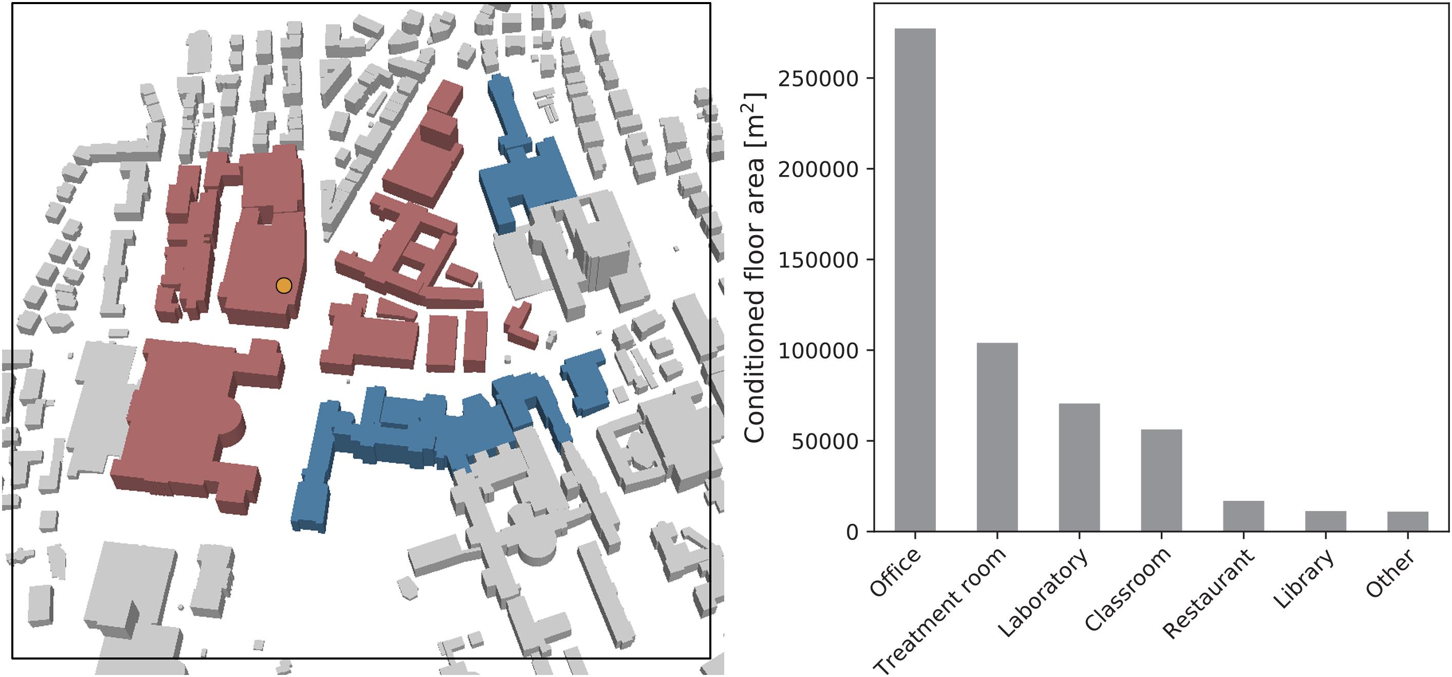
Figure 3. Aerial representation of the case study area and functional distribution of the buildings under consideration. The functions shown as “Office” include both research and hospital spaces. The buildings selected for this study are colored red for university buildings and blue correspond to the hospital. The yellow circle marks the location of the temperature sensor in the case study area.

The importance of the climatic environment in relation to energy-efficient solutions is expected to increase in view of climate change. During a heat wave in 2015, a difference of up to 5 K was observed between urban and rural weather stations in Zurich, and even a slightly positive UHI during the daytime was found (Mussetti et al., 2019). Several studies have estimated the impact of increased temperatures on Swiss energy demand (Frank, 2005; OcCC and ProClim, 2007; Gonseth et al., 2017), stating that while the number of heating days is expected to decline, the number of cooling days will grow significantly, with a consequent increase in energy demand for space cooling. In the Swiss central plateau where Zurich is located, annual cooling energy consumption for office buildings in the scenarios analyzed by Frank (Frank, 2005) is calculated to rise by 223–1050%, while annual heating energy consumption is expected to fall by 36–58%.

In order to assess the effects of such extreme weather events on the district’s energy demands, we selected two consecutive hot days with clear sky during the heat wave that affected Zurich in 2015 (2–3 July 2015). For the selected period, two climate datasets were prepared. The Baseline climate dataset was obtained from Meteonorm (Meteotest, 2014) and uses data from the offsite weather station SMA. The Microclimate dataset was obtained through ENVI-met simulations and was validated by comparing the simulated air temperature to measured data from a roof sensor within the case study area. Spatial data for the case study area, comprising the topography, building footprints and number of floors, were retrieved from local GIS data and the from the Federal Register of Buildings and Dwellings (Bundesamt für Statistik, 2010).

Baseline Climate Dataset

The Baseline climate dataset is derived from measured data from the national weather station SMA, located in Zurich Fluntern, 1.35 km uphill from the area. This dataset is employed both as an input to the ENVI-met simulation and as climatic boundary conditions to model energy demand in CEA for the Baseline case.

The selected days (2–3 July 2015), during which Zurich was affected by a heat wave event, are selected as representative extreme hot days. As shown in Figure 4, the two days reach temperatures higher than 30°C and humidity values above 70%. During both days, the maximum diurnal temperature is registered at around 33°C, while the night temperature is lower at around 20°C for the first day and 22°C during the second day. As clear sky and no rain were filtering parameters for the selection of the period, the daily humidity pattern appears similar during the two days, ranging between 35% and 80%. Wind velocity reaches a maximum speed of 3.3 m/s and wind speed below 1 m/s is registered generally between sunset and sunrise.

FIGURE 4

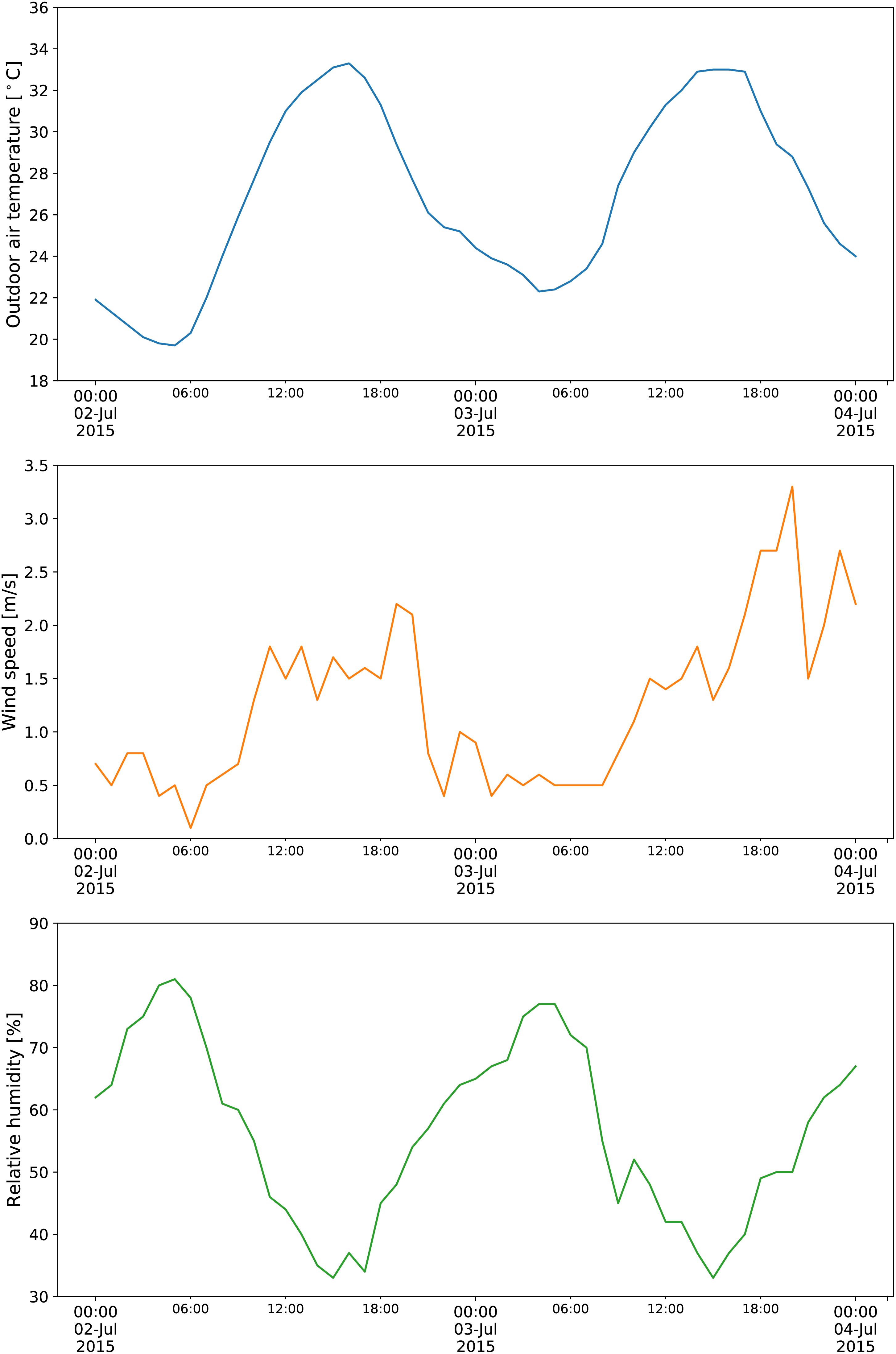
Figure 4. Data from the weather station SMA for the time period under analysis.

Microclimate Dataset: ENVI-met Model Construction and Parameters

The second dataset is obtained by validated ENVI-met simulations and reports the specific thermodynamic characteristics of the Hochschulquartier district. After an iterative calibration process of building and paving materials, two simulations were performed with different grid resolutions. The following section reports ENVI-met inputs and simulation settings.

Table 1 summarizes the input parameters used for the ENVI-met model subdivided into the categories of Area Input file and Configuration file. To obtain reliable simulation results for the area of interest it is necessary to model a larger area. This is because the urban surrounding influences the microclimate in the area of interest, but also because microclimate models do not work reliably at the model borders. In this case study, a first boundary has been drawn around the area of interest including adjacent street canyons and adjoining building façades. From this border an offset area of 100 m was taken as the area of influence (as seen in Figure 3) as a conservative assumption (Wong et al., 2012).

TABLE 1

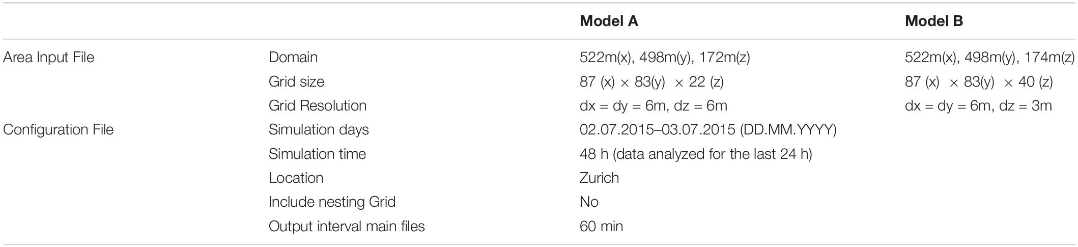
Table 1. ENVI-met model settings.

As the process of validation was complemented by a mesh sensitivity analysis, two Area Input Files were created using a grid cell unit of 6 m (x) by 6 m (y) by 6 m (z) -Model A-, and 6 m (x) by 6 m (y) by 3 m (z) -Model B-, respectively. On the horizontal plane, to cover the area of study plus the area of influence, 87 cells were set for the x axes and 83 cells for the y axes. Regarding the z axis, the height of the model was calculated as the sum of maximum topographic elevation and the height of the tallest building in the district (55 m). In order to avoid computational instability due to proximity of objects to the upper domain limit, the height of the domain was doubled. As the mesh sensitivity explores the variation in vertical resolution the number of z cells was therefore set to 22 for Model A, and 40 for Model B, using a telescopic factor of 20% (from 90 m upward).

Once the domain was defined, the 3D model of the Hochschulquartier was built. Detailed spatial data, collected by survey, was used to build a database in the appropriate formats required by the tool. The database includes topographical information, building geometry and materials, tree position and height, and surface cover. For some of the retrieved data, a process of classification allowed to reduce complexity while preserving the main characteristics of the district, i.e., building materials were classified in four categories according to the building’s construction year and construction type, while trees were classified on the basis of height and leaf area density (Table 2). Moreover, two surface/soil materials, one for impervious (asphalt) and one for pervious surfaces (loamy soil), were used from the ENVI-met default Database (Table 3).

TABLE 2

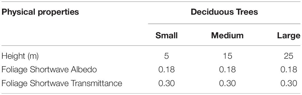
Table 2. Physical properties of the vegetation used in the ENVI-met model.

TABLE 3

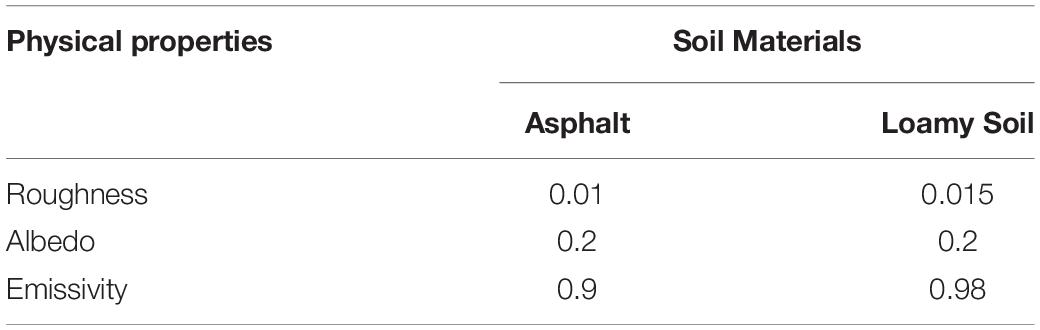
Table 3. Physical properties of the soil materials used in the ENVI-met model.

Table 4 shows the characteristics of the materials employed for the simulations in detail. ENVI-met simulations are performed using the full forcing method and employing weather data for the selected days from the SMA weather station. Hourly data of dry bulb temperature and relative humidity (shown in Figure 4) as well as the hourly average wind speed and predominant wind direction were used as forcing climate variables. The day under analysis was 3 July 2015, a hot day with clear sky. Taking into account initialization time, the simulation started at 00:00:01 on July 2 and had a duration of 48 h. Only the values of the last 24 h were then selected for the analysis. Simulations were carried out for Model A and B with the described settings. The validated model with higher level of accuracy will be selected and passed to CEA for the building energy demand simulation in the Microclimate case.

TABLE 4

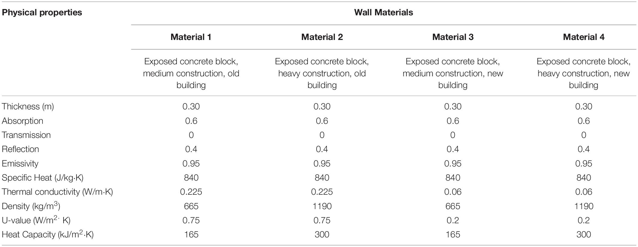
Table 4. Physical properties of the wall materials used in the ENVI-met model.

CEA Database and Model Construction

The inputs to the CEA energy demand model comprise a set of primary and secondary inputs. The primary inputs to the simulation must be provided by the user as an input and correspond to the geometry, functional mix, and construction and renovation years for each building in the district. As previously mentioned, the spatial data for the Hochschulquartier case study area, such as the topography and building footprints, were retrieved from local GIS data. The number of floors and the construction year of each building were obtained from the Federal Register of Buildings and Dwellings (Bundesamt für Statistik, 2010). Each building’s functional mix was derived from building catalogs obtained from the institutions that operate them, namely ETH Zürich and the University Hospital Zürich, as shown in Figure 3.

In order to reduce the amount of data that needs to be collected for individual buildings, the secondary inputs to CEA may be supplied by the user where available, or otherwise derived from the CEA archetype database (Fonseca and Schlueter, 2015), which contains typical construction properties for a variety of building functions and construction years. These inputs include the thermal properties of the building envelope, building systems and controls, occupancy schedules, internal gains from occupant activities and electricity use, as well as the indoor comfort setpoints. For the present study, window-to-wall ratios were estimated based on the actual characteristics of the buildings, while construction materials from the CEA archetype database were adapted in order to match the inputs required for the ENVI-met simulation (Table 4) and assigned to individual buildings based on their construction year. All other inputs were derived from the CEA archetype database for the corresponding construction years and building functions. The most relevant secondary input parameters used in the model of the Hochschulquartier are summarized in Table 5.

TABLE 5

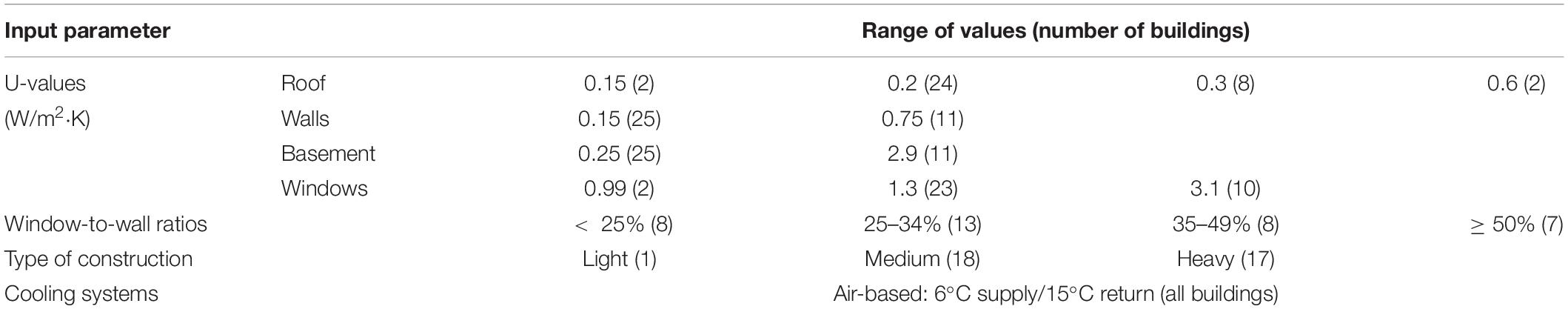
Table 5. CEA model settings used in the case study.

While CEA includes a stochastic occupancy model (Mosteiro-Romero et al., 2020), the simpler standard-based deterministic schedules of occupant presence and electricity consumption were used in this study in order to isolate the effects of microclimate from changes in occupancy patterns. As discussed in section “Wind Speed Effects on Air Infiltration,” the CEA dynamic infiltration model was used and a dynamic convective heat transfer model was added to the software in order to fully capture the effects of wind speed on the predicted demands of the district.

Results

The following sections describe the results from the microclimate simulation and its consequent effects on the predicted space cooling demand for the case study area. In the first section, ENVI-met results are validated by comparing the simulated air temperature on the roof of a building in the case study area to measured data from a sensor on the roof of that building. The local microclimate is then characterized by comparison to the data from the off-site weather station SMA. The CEA simulation results for space cooling demand for the Baseline case using weather station data are compared to the Microclimate case using ENVI-met results as an input.

Validation of the ENVI-met Model

In order to validate the results of the microclimate model obtained through ENVI-met, the simulated results are compared to field measurements. This process allows to evaluate the model accuracy and the reliability of the input data. A temperature sensor positioned on the roof of the Maschinenlaboratorium (ML) building, located within the case study area (Figure 3), provides measured data for the period studied with a time interval of 15 min.

A mesh sensitivity analysis is performed to estimate the accuracy of ENVI-met while changing the height resolution. This analysis consists of the comparison of the simulation results between two models with a respective resolution of 6 m(x) × 6 m(y) × 6 m (z) (Model A) and 6 m(x) × 6 m(y) × 3 m (z) (Model B) for 2–3 July. Simulation data for the comparison is extracted at the same height as the actual temperature sensor.

Figure 5 compares the hourly evolution of measured temperature with ENVI-met modeled temperatures. Results show a similar pattern between simulated and monitored data and good stability of ENVI-met concerning the sensitivity to cell height resolution. However, for both models, the simulated air temperature is higher than the measured air temperatures during daytime hours with an absolute maximum divergence of 1.9°C (Model B) and 2.3(°C (Model A). As the change in mesh resolution shows minor variations in the computation of air temperature values, a comparison of the Mean Absolute Error (MAE) is employed to estimate the average of the absolute residual values. As Model B presents slightly lower MAE value (0.80) than Model A (0.91), the simulation results from Model B are used as boundary climate conditions for the Microclimate Case in CEA.

FIGURE 5

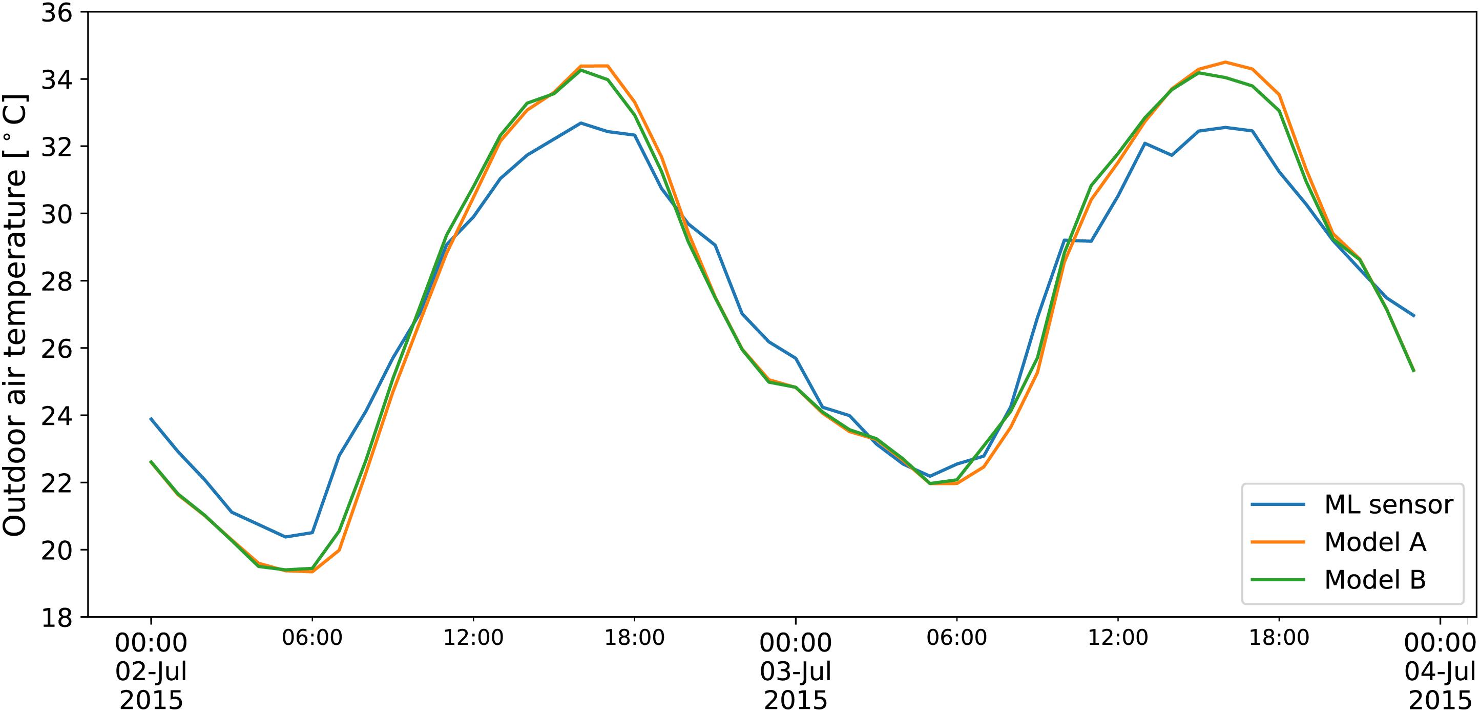
Figure 5. Outdoor air temperature results from the microclimate simulations for Model A and Model B compared to measured data from the sensor on the ML building.

Before passing the data to CEA, the accuracy of the ENVI-met model performance is examined through few parameters, usually applied to ensure the reliability of the simulations’ outputs (Tsoka et al., 2018)[59]. For this purpose, a linear covariance correlation (R2) is carried out. As statistically significant values of R2 are often unrelated to the magnitude of differences between observations and predictions (Willmott, 1983)[60], the Root Mean Square Error (RMSE), which describes the magnitude of mean differences between observed and predicted values, and the index of agreement (d), which indicates the degree of model prediction error, were determined additionally.

The model is considered reliable when R² and d both tend to 1 and RMSE tends to 0. The measured parameters show that the simulation results are highly accurate, with a R² of 0.97, d index of 0.98 and a RMSE of 1.02°C. Thus, the comparison confirms that ENVI-met has simulated atmospheric temperature in the studied area with good accuracy. However, the model tends to overestimate daytime temperature up to 2°C and a divergence of this magnitude might have repercussions on energy demand estimation.

Microclimate Characteristics of the Hochschulquartier

The radiative, aerodynamic and thermal properties of urban materials lead to microclimatic processes that are reflected in the distinct formulation of the Surface Energy Balance (SEB) for rural and urban systems. In particular, the SEB of cities is influenced by the larger heat storage capacity of urban materials, and thermal exchanges between built surfaces and the atmosphere. Urban materials and geometric characteristics contribute to the local climate performance of the district by influencing solar access, radiative absorption and friction to wind flows. Such a performance is examined here based on the ENVI-met results of air temperature, relative humidity, and wind speed. The overall microclimate profile of the Hochschulquartier is observed by analyzing averaged hourly values for the full district, while a more detailed spatial analysis allows the understanding of microclimate patterns and the local climate context of each building in the district.

For the analysis of the Hochschulquartier microclimate profile, values around building envelopes are obtained from ENVI-met results for air temperature, wind speed and relative humidity. Aggregated district data reporting average values are then compared to the Baseline climate values, used as boundary conditions for the simulation. Figure 6 shows that local temperatures are generally around 0.7°C lower during night-time and 1.2°C higher during daytime compared to Baseline temperatures. The maximum variation is reached during the warmest hours when the local temperature increases till 34°C.

FIGURE 6

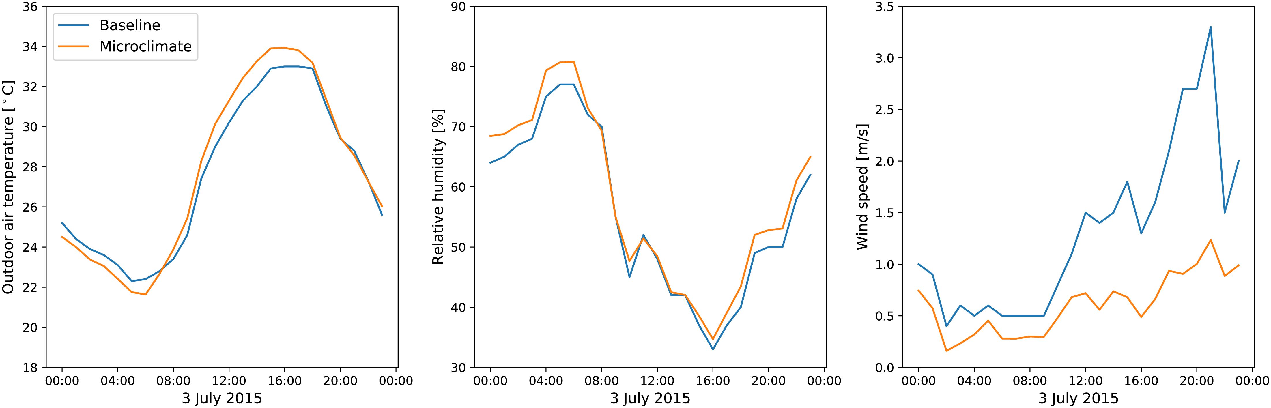
Figure 6. Simulated mean air temperature, relative humidity and wind speed in the area compared to data from Baseline climate values.

The simulation results show slightly higher values than the Baseline regarding relative humidity, however, minor variations are observed during the warmest hours of the day. As processes of evapotranspiration and evaporation are usually enhanced by solar radiation, this pattern suggests that the presence of unpaved surfaces and greening gives a minor contribution to the moisture level of the Hochschulquartier. Thus, higher values of local relative humidity during night hours might be influenced by lower temperatures and by lower wind velocity in the district that prevent humidity dispersion. Additionally, the average wind speed around the buildings compared to the Baseline shows a relevant decrease in velocity during the second half of the day. This suggests that the roughness elements such as buildings and trees generally contribute to lowering the wind velocity; wind speeds are below 1.3 m/s in the Hochschulquartier while the meso-scale wind velocity reaches 3 m/s.

Moreover, the observation of the Hochschulquartier results, visualized through the ENVI-met visualization tool Leonardo, highlights daily microclimate patterns on the horizontal dimension. To better describe the distribution of thermal and ventilation effects, three representative hours for the morning, afternoon and night patterns are selected. Figure 7 shows the distribution of ambient temperature values in the district. Relevant variations, in the range of 4°C, are observed during daytime. While during morning hours higher values are registered in the central part of the district, during afternoon hours the west part results to be consistently warmer, reaching 38°C. The west part also has a lower absorption capacity than the east part since during night hours temperature values quickly decrease inverting the daytime pattern. However, the difference in temperature during the night-time is lower, at around 1°C.

FIGURE 7

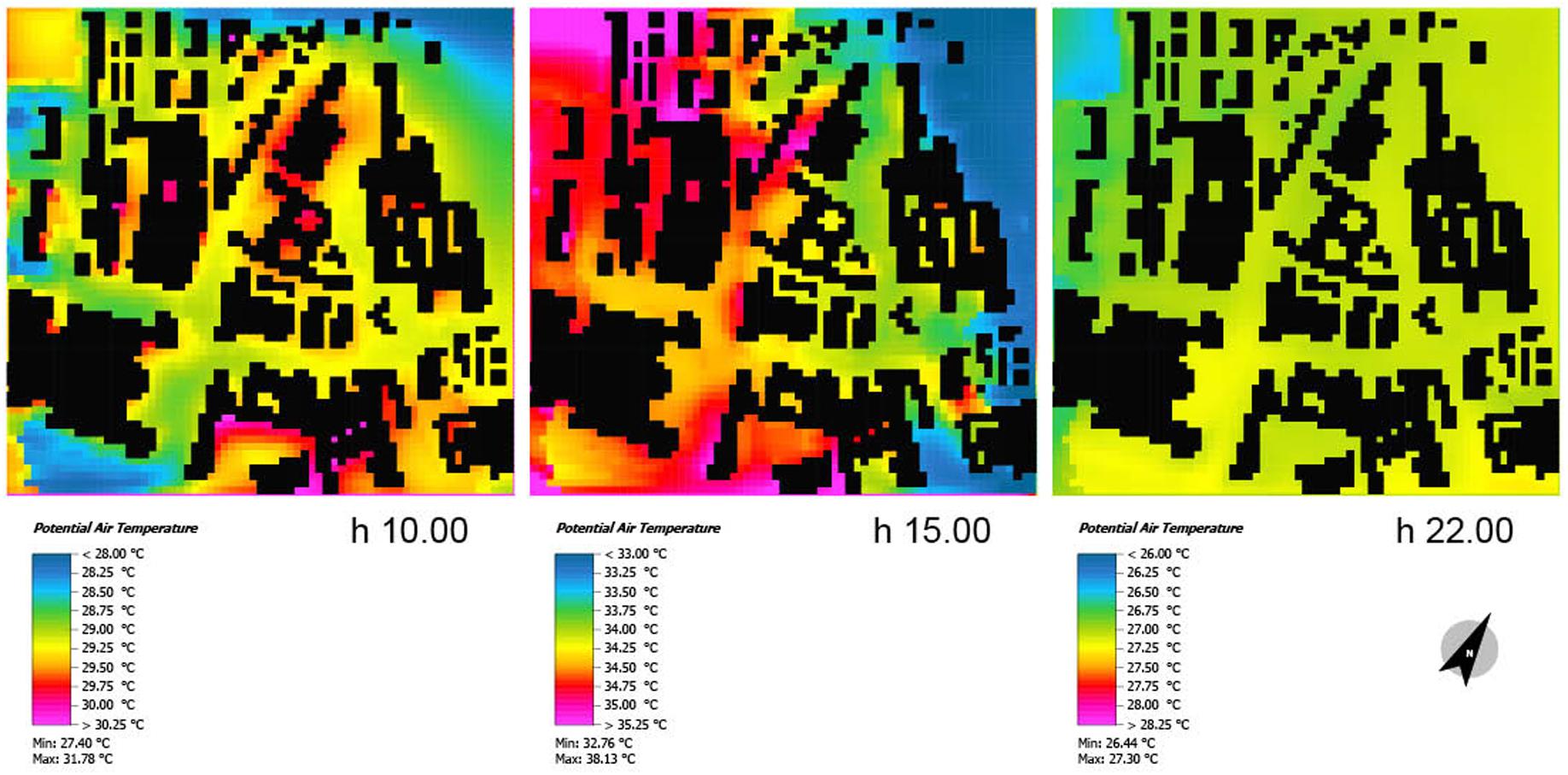
Figure 7. Spatial distribution of air temperature at 2 m height.

Figure 8 shows wind velocity results for three hours that were found to be representative of the wind flow distribution in the area. Generally, the spatial visualization confirms the overall microclimate profile indicating that the roughness level of the district significantly lowers wind velocity. However, some variations can be observed concerning the southern part of the area. Here the main street canyons generally show higher wind velocities than the rest of the district during day and night hours. In particular, the street with direction east-west sees an increase in flow velocity from 0.75 m/s in the morning to 2 m/s in the night. This pattern seems to be a function of the meso-scale input, suggesting that the southern street canyons are most influenced by changes in meso-scale wind flows.

FIGURE 8

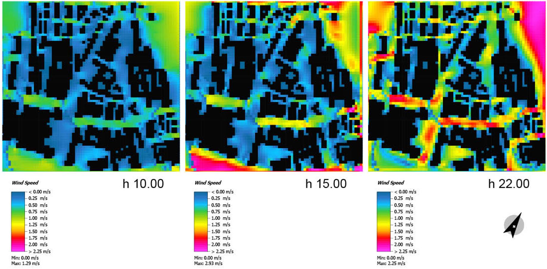
Figure 8. Spatial distribution of wind speed at 2 m height.

Finally, Figure 9 shows the hourly results for air temperature, relative humidity and wind speed around each building under analysis. These values have been used as boundary climate conditions in the CEA simulation for the Microclimate case. The differences observed between buildings confirm the previous spatial analysis that showed significant variations within the area and distribution patterns during day and night-time, in particular regarding wind speed.

FIGURE 9

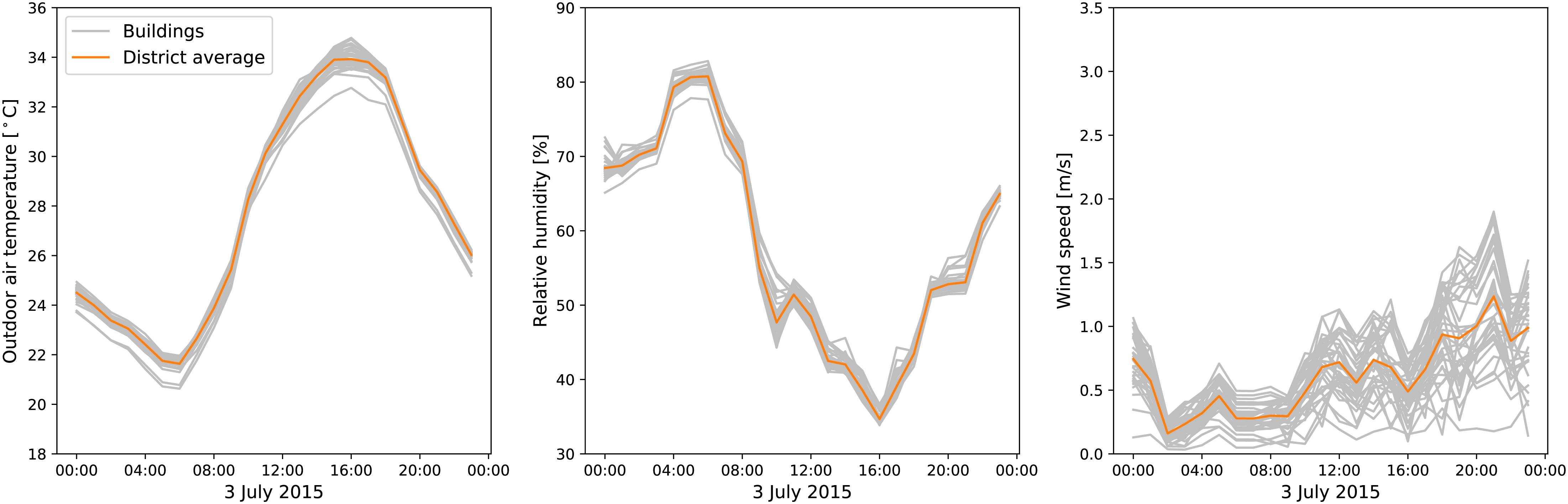
Figure 9. Simulated mean air temperature, relative humidity and wind speed around buildings.

Comparison of the Space Cooling Demand for Each Weather Case

The district’s space cooling demand was simulated in CEA using the Baseline climate dataset and the microclimate simulation results from ENVI-met for the day being analyzed (3 July 2015). The distribution of the predicted space cooling demand for each building on the selected day is shown in Figure 10. The results show that the cooling demands in the area are dominated by sensible cooling, meaning that air dehumidification contributes a comparatively lower share of the total cooling demand in the district. Accounting for local microclimate in the simulations leads to an increase in the daily and peak demands for both latent and sensible cooling. The results for the peak latent cooling show a smaller spread for the Microclimate case, with a higher average value but a lower maximum.

FIGURE 10

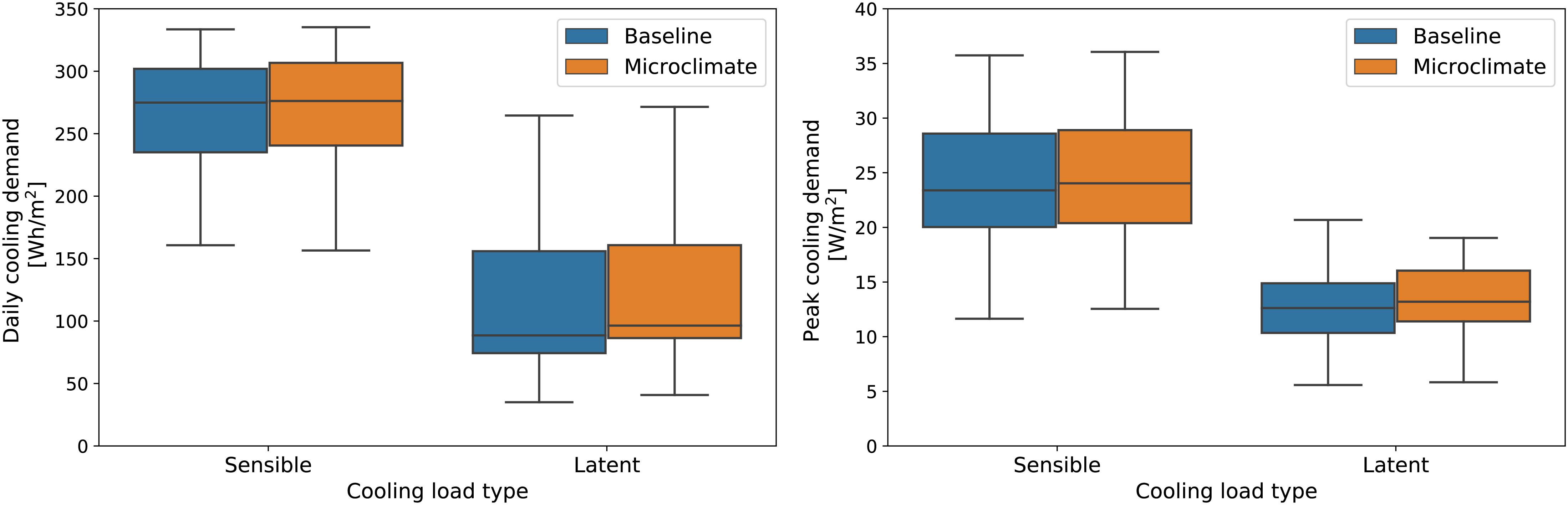
Figure 10. Box plots showing the space cooling demand and peak cooling power on the selected day when using weather station data compared to using local microclimate simulations. The total space cooling demand comprises the sensible and latent demands.

In relative terms, as shown in Figure 11, accounting for local microclimate leads to a 5% increase in the district’s space cooling demand on this day, with a maximum increase of 14% for one of the buildings. The effects are even more visible on the peak demands, where the use of simulated microclimate data leads to an average increase of 8% in the peak cooling power required by the buildings in the district. The peak cooling demand is increases by up to 15%.

FIGURE 11

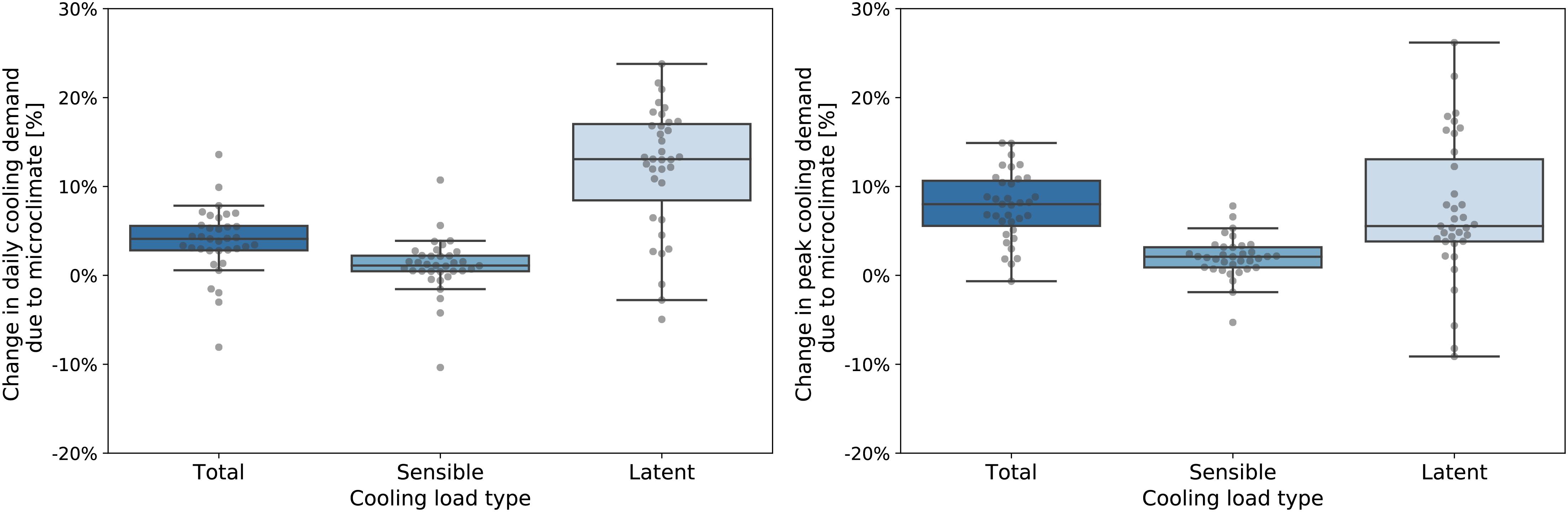
Figure 11. Box plots showing the change in space cooling demand and peak cooling power on the selected day when replacing the weather station data with simulated local microclimate results. The total space cooling demand comprises the sensible and latent demands.

The increase in space cooling demand is mainly caused by latent cooling, which increases by 11% for the entire district. This is due to both the increase in relative humidity when accounting for microclimate as well as the overall lower wind speeds in the area. Since wind speed affects the infiltration rate in individual buildings, the required ventilation rate is also affected by local low wind velocity, as discussed in section “Wind Speed Effects on Air Infiltration.” The overall lower wind speeds in the district lead to lower air infiltration, which in the CEA calculation leads to increased ventilation rates and thus the amount of air that needs to be dehumidified also increases. This is further demonstrated by the large spread in the variation in latent cooling demand, and particularly for the peak latent cooling load. The large variations in wind speed around individual buildings observed in Figure 9 leads to varying ventilation rates in different buildings, and hence the latent cooling loads vary from building to building.

However, a few outliers for which the cooling demand actually decreases when including microclimate are also encountered. This effect can be explained by analyzing the hourly results, shown in Figure 12. The area has a distinct cooling load pattern that closely follows the occupancy and lighting schedules in the buildings, with two peaks and a valley during the middle of the day as building occupants leave their work spaces for lunch. When accounting for the effects of urban microclimate, the overall cooling demand is higher during the second peak due to the increased outdoor air temperatures, leading to an overall higher cooling peak for the district. However, the cooling demand is lower in the morning peak due to the lower latent cooling in the morning hours. At least one of the buildings has its peak cooling demand at 10 in the morning in the Baseline case. At this time, however, the distribution in the cooling loads for the buildings in the area is drastically smaller in the Microclimate case. Hence, some buildings have lower peak cooling demands on the selected day due to the lower morning peak.

FIGURE 12

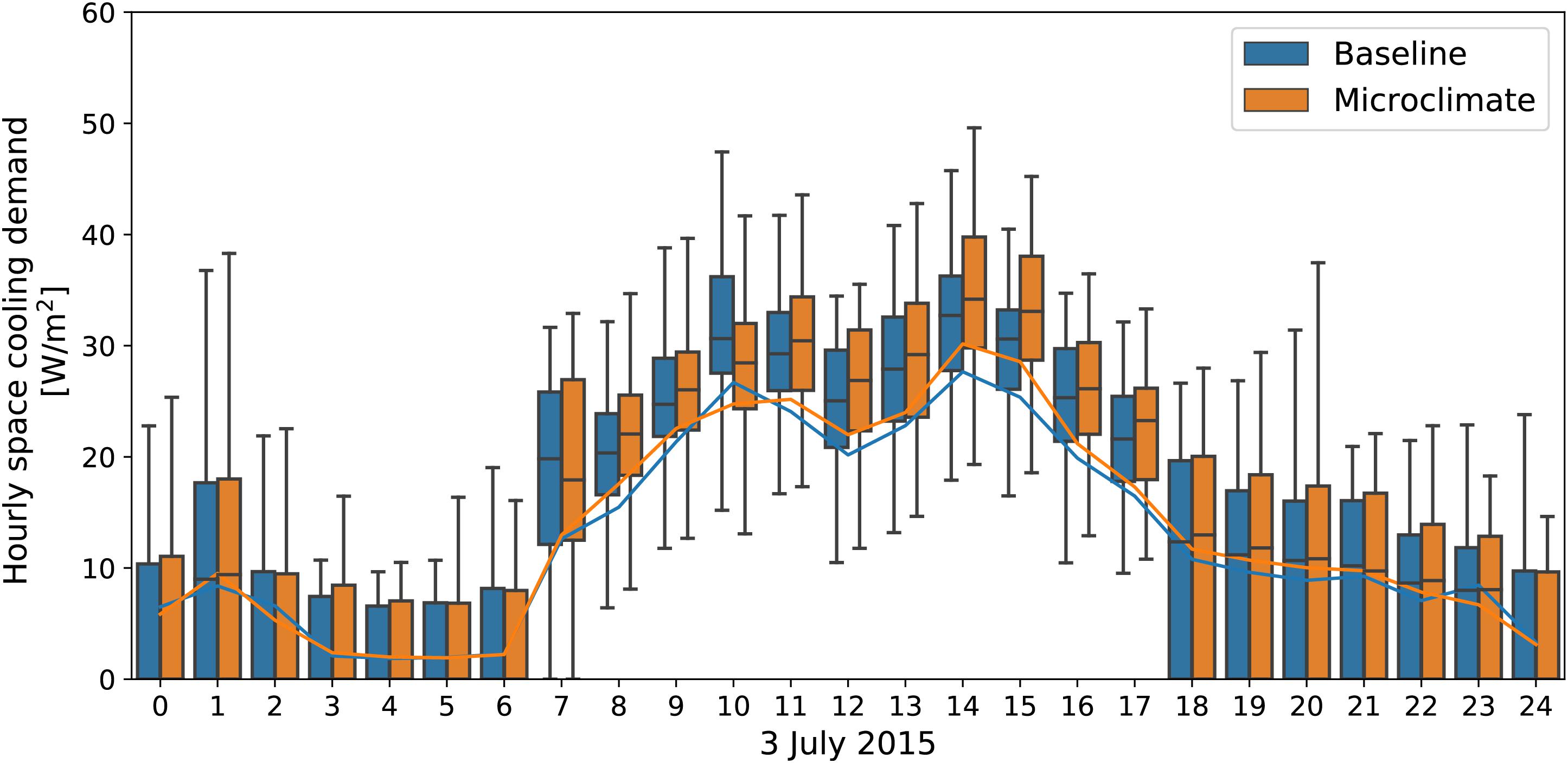
Figure 12. Hourly space cooling demand in the district on the selected day for each of the climate cases. The boxplots at each hour show the distribution in the space cooling demand per conditioned floor area for all buildings in the area, whereas the lines show the entire district’s demand per square meter for each case.

The deviation for individual buildings is shown spatially in Figure 13. The results show that the change in daily space cooling demand is greatest for a large historical building in the area. This building includes sports facilities, and therefore require a significant amount of cooling and dehumidification. Furthermore, as an older building the infiltration rate is large, thus the aforementioned variation in wind speed has a particularly large effect for this building. The increase in the peak cooling demand, on the other hand, is greatest for hospital buildings, concentrated on the eastern part of the district. Relative decreases in space cooling demand are comparatively smaller and mostly correspond to smaller buildings.

FIGURE 13

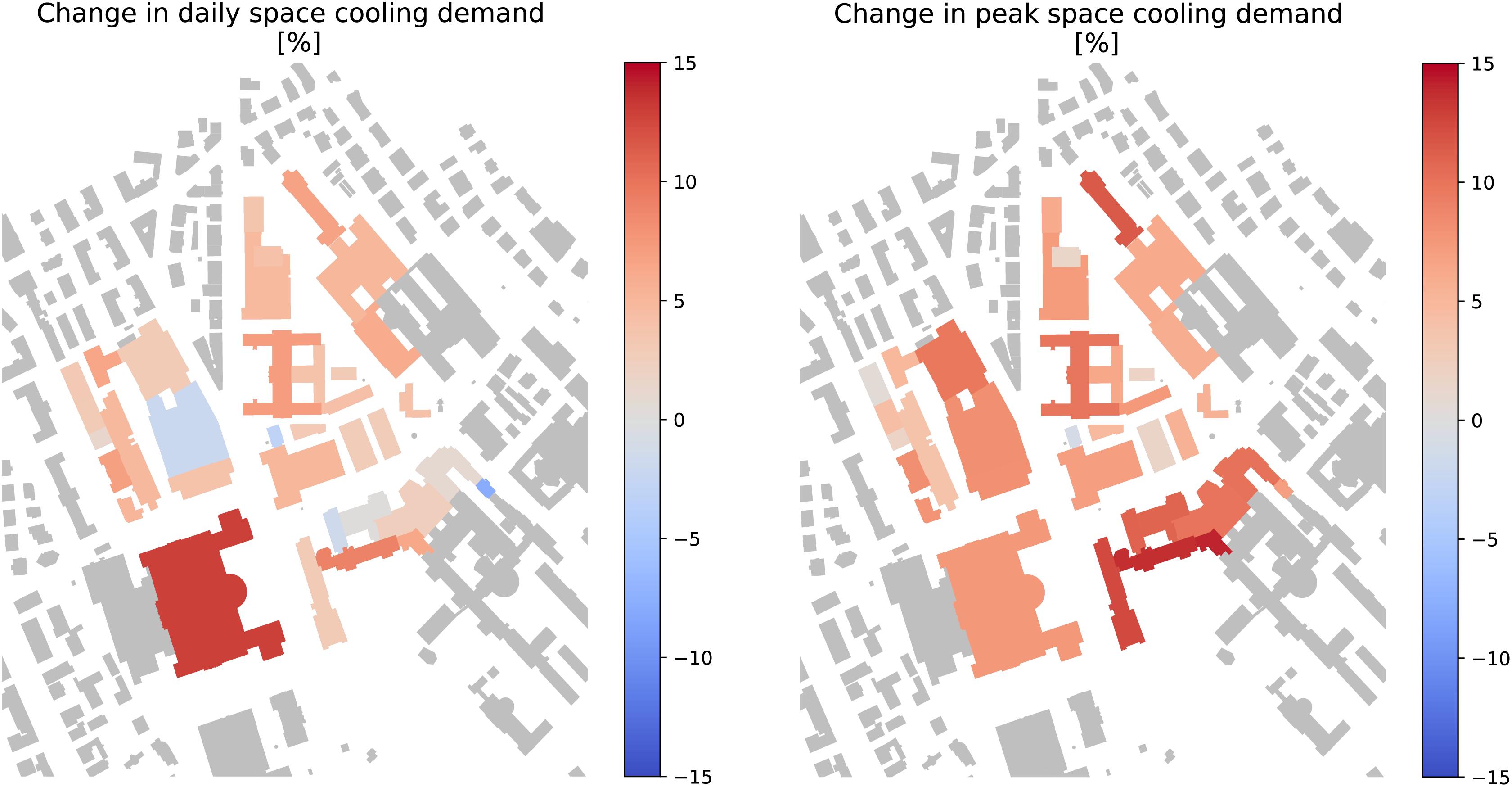
Figure 13. Change in total and peak cooling demand on the selected day due to the effect of microclimate for each building in the area.

Limitations

The proposed method represents a promising new approach to analyze the mutual interactions between buildings and microclimate in urban districts. Regarding the application of the method on the Hochschulquartier district, the study has shown significant variations in cooling demand between a Baseline and a Microclimate case, confirming the findings of previous studies regarding the increase of cooling loads when local climate phenomena are taken into account in the energy assessment (Santamouris, 2014; Li et al., 2019). However, in the energy simulations the microclimate profile of the area was compared to the Baseline climate data derived from an offsite weather station in Zurich Fluntern. Since the weather station is located in a suburban area the magnitude of the UHI phenomena is not fully captured. Thus, the use of rural weather data for the Baseline energy scenario would likely result in higher variations of cooling loads between the two cases.

The applicability of the method is furthermore somewhat limited by the extremely high computational costs, in particular for running ENVI-met simulations. In the present work, a one-way integration method was investigated, whereby urban microclimate affected energy performance, but buildings’ energy consumption did not affect microclimate. However, given the feedback loop created between urban microclimate, buildings’ energy performance, building surface temperatures and heat emissions from cooling systems, an iterative simulation method would be required to fully capture these mutual effects, however, this would further explode the computational expense of the method.

While the method permits the exploration of different coexisting geometries, materials, energy systems and the analysis of their effects during extreme weather events, planning energetic interventions based on analyzing patterns observed during a single day is not recommended. The implementation of this methodology during the design process might thus hinge on the further development of less computationally expensive methods to provide high-resolution simulations of local climate in urban areas. Further work needs to be carried out to expand the time scale of urban microclimate simulations without losing spatial resolution in order to support design assessment and energy demand simulations.

Conclusions

The study outlines a method for quantitative analysis of district-scale energy consumption taking into account the microclimatic effects created by the design of open and built space. The study constitutes a first attempt at coupling microclimate and building energy modeling tools at the district scale. The method applied to a case study in Zurich, Switzerland showed that the coupled tools can deal with complex geometrical, material and behavioral features. Validated ENVI-met results were used to analyze microclimate patterns in the case study for a hot summer day during a heat wave. The space cooling demand for the buildings in the area was modeled in the City Energy Analyst (CEA) in order to assess the district’s energy performance when accounting for the local microclimate. Results were compared to a second energy demand simulation using measured data from an offsite weather station.

For the exemplary case study, the urban microclimate model showed good agreement with the measured data available in the district analyzed. The comparison between Microclimate and Baseline climate values showed that mean local air temperature was generally higher during daytime in a range of 1.2°C, while humidity was higher during night hours. However, when analyzing more in detail the spatial distribution of microclimate variables it is possible to observe that during the daytime the west part of the district was significantly warmer than the east part and temperature rapidly decreased during night-time. This thermal pattern suggests a relatively low absorption capacity of the western part of the district influenced by material characteristics and urban form. In addition, the roughness level of the district contributes to lower local mean wind velocity, which was below 1.3 m/s throughout the day, while a relative increase in wind speed and turbulence is observed along the street canyons in the south part of the district.

While the increased air temperatures due to local microclimate led to an increase in the sensible cooling demand in the case study area, the increased relative humidity and the high variance in the local wind speed led to an even greater change in the latent cooling demand. Overall, the district’s space cooling demand on the selected day was found to increase by 5% when considering local microclimate, with an average increase in the peak cooling demand of 8%. Moreover, the coupling method allowed a detailed analysis of the different effects microclimate can have on buildings’ energy, showing that, when considering the local climate patterns, space cooling demand on the selected day varied between −5% and +14%.

The results indicate the capacity of the integrated method to depict the influence of microclimatic conditions on the cooling demand in an urban district. By expanding the scope from the single-building to the district scale, the method can be used to explore the mutual thermal and aerodynamic influence between buildings, and the consequent impact on the cooling loads at both the building and the district scale. In particular, the fine resolution of the results allows a deep understanding of the variation in performance of single buildings depending on local climate patterns of ambient temperature, relative humidity and wind velocity. Therefore, the method can support the challenge of improving building energy efficiency by offering an assessment instrument that integrates form configuration, materials and consequent microclimate factors.

Further consideration should be given to the possible employment of this method during the design process and not only as an assessment instrument. In the current study, an existing district was modeled in order to validate the microclimate simulations against measured data. Future studies could use the proposed methodology to further explore the effects of design decisions on future districts’ performance as well as to test the potential for urban form interventions to mitigate the urban heat island and reduce cooling demand.

Data Availability Statement

The raw data supporting the conclusions of this article will be made available by the authors, without undue reservation.

Author Contributions

MM-R and DM contributed equally to this work and are co-main authors of this article. MP-vE and AS provided guidance and support to the main authors of the manuscript. All authors contributed to the article and approved the submitted version.

Funding

This research was developed as part of the project SPACERGY, within the JPI Urban Europe research framework. The work presented in this paper was financed by the Swiss Federal Office of Energy (SI/501404-01) and the Netherlands Organisation for Scientific Research (NWO 438.15.413).

Conflict of Interest

The authors declare that the research was conducted in the absence of any commercial or financial relationships that could be construed as a potential conflict of interest.

References

Ali-Toudert, F., and Mayer, H. (2006). Numerical study on the effects of aspect ratio and orientation of an urban street canyon on outdoor thermal comfort in hot and dry climate. Build. Environ. 41, 94–108. doi: 10.1016/J.BUILDENV.2005.01.013

CrossRef Full Text | Google Scholar

Ali-Toudert, F., and Mayer, H. (2007). Effects of asymmetry, galleries, overhanging façades and vegetation on thermal comfort in urban street canyons. Solar Energy 81, 742–754. doi: 10.1016/j.solener.2006.10.007

CrossRef Full Text | Google Scholar

Allegrini, J., Dorer, V., and Carmeliet, J. (2012). Influence of the urban microclimate in street canyons on the energy demand for space cooling and heating of buildings. Energy Build. 55, 823–832. doi: 10.1016/j.enbuild.2012.10.013

CrossRef Full Text | Google Scholar

Allegrini, J., Orehounig, K., Mavromatidis, G., Ruesch, F., Dorer, V., and Evins, R. (2015). A review of modelling approaches and tools for the simulation of district-scale energy systems. Renew. Sustain. Energy Rev. 52, 1391–1404. doi: 10.1016/j.rser.2015.07.123

CrossRef Full Text | Google Scholar

Baudirektion Kanton Zürich (2014). Masterplan Hochschulgebiet Zürich-Zentrum. Zurich: Zentrum University.

Google Scholar

Blocken, B. (2014). 50 years of computational wind engineering: past, present and future. J. Wind Eng. Indust. Aerodyn. 129, 69–102. doi: 10.1016/j.jweia.2014.03.008

CrossRef Full Text | Google Scholar

Bruse, M., and Fleer, H. (1998). Simulating surface-plant-air interactions inside urban environments with a three dimensional numerical model. Environ. Model. Softw. 13, 373–384. doi: 10.1016/S1364-8152(98)00042-5

CrossRef Full Text | Google Scholar

Bundesamt für Statistik (2010). Eidgenössisches Gebäude- und Wohnungsregister. Neuchâtel: Bundesamt für Statistik (BFS).

Google Scholar

Carnielo, E., and Zinzi, M. (2013). Optical and thermal characterisation of cool asphalts to mitigate urban temperatures and building cooling demand. Build. Environ. 60, 56–65. doi: 10.1016/J.BUILDENV.2012.11.004

CrossRef Full Text | Google Scholar

The CEA Team (2018). City Energy Analyst v2.9.0. Zenodo. doi: 10.5281/zenodo.1487867

CrossRef Full Text | Google Scholar

Cui, Y., Yan, D., Hong, T., and Ma, J. (2017). Temporal and spatial characteristics of the urban heat island in Beijing and the impact on building design and energy performance. Energy 130, 286–297. doi: 10.1016/j.energy.2017.04.053

CrossRef Full Text | Google Scholar

DIN EN 16798-7 (2015). Energieeffizienz von Gebäuden – Berechnungsmethoden zur Bestimmung der Luftvolumenströme in Gebäuden inklusive Infiltration. Berlin: Deutsches Institut für Normung.

Google Scholar

Eurostat (2016). Urban Europe – Statistics on Cities, Towns and Suburbs. Luxembourg: European Union.

Google Scholar

Fonseca, J., and Schlueter, A. (2015). Integrated model for characterization of spatiotemporal building energy consumption patterns in neighborhoods and city districts. Appl. Energy 142, 247–265. doi: 10.1016/j.apenergy.2014.12.068

CrossRef Full Text | Google Scholar

Frank, T. (2005). Climate change impacts on building heating and cooling energy demand in Switzerland. Energy Build. 37, 1175–1185. doi: 10.1016/J.ENBUILD.2005.06.019

CrossRef Full Text | Google Scholar

Frayssinet, L., Merlier, L., Kuznik, F., Hubert, J., Milliez, M., and Roux, J. (2018). Modeling the heating and cooling energy demand of urban buildings at city scale. Renew. Sustain. Energy Rev. 81, 2318–2327. doi: 10.1016/j.rser.2017.06.040

CrossRef Full Text | Google Scholar

Gobakis, K., and Kolokotsa, D. (2017). Coupling building energy simulation software with microclimatic simulation for the evaluation of the impact of urban outdoor conditions on the energy consumption and indoor environmental quality. Energy Build. 157, 101–115. doi: 10.1016/j.enbuild.2017.02.020

CrossRef Full Text | Google Scholar

Gonseth, C., Thalmann, P., and Vielle, M. (2017). Impacts of global warming on energy use for heating and cooling with full rebound effects in Switzerland. Swiss J. Econ. Statist. 153, 341–369. doi: 10.1007/BF03399511

CrossRef Full Text | Google Scholar

Gros, A., Bozonnet, E., and Inard, C. (2014). Cool materials impact at district scale – coupling building energy and microclimate models. Sustain. Cit. Soc. 13, 254–266. doi: 10.1016/j.scs.2014.02.002

CrossRef Full Text | Google Scholar

Gros, A., Bozonnet, E., Inard, C., and Musy, M. (2016). Simulation tools to assess microclimate and building energy – A case study on the design of a new district. Energy Build. 114, 112–122. doi: 10.1016/j.enbuild.2015.06.032

CrossRef Full Text | Google Scholar

Guattari, C., Evangelisti, L., and Balaras, C. (2018). On the assessment of urban heat island phenomenon and its effects on building energy performance: a case study of Rome (Italy). Energy Build. 158, 605–615. doi: 10.1016/j.enbuild.2017.10.050

CrossRef Full Text | Google Scholar

Happle, G., Fonseca, J., and Schlueter, A. (2017). Effects of air infiltration modeling approaches in urban building energy demand forecasts. Energy Proc. 122, 283–288. doi: 10.1016/j.egypro.2017.07.323

CrossRef Full Text | Google Scholar

He, J., Hoyano, A., and Asawa, T. (2008). A numerical simulation tool for predicting the impact of outdoor thermal environment on building energy performance. Appl. Energy 86, 1596–1605. doi: 10.1016/j.apenergy.2008.12.034

CrossRef Full Text | Google Scholar

Hirano, Y., and Fujita, T. (2012). Evaluation of the impact of the urban heat island on residential and commercial energy consumption in Tokyo. Energy 37, 371–383. doi: 10.1016/j.energy.2011.11.018

CrossRef Full Text | Google Scholar

Huttner, S. (2012). Further Development and Application of the 3D Microclimate Simulation ENVI-Met. Mainz: University of Mainz.

Google Scholar

ISO 52016-1 (2017). Energy Performance of Buildings – Energy Needs for Heating and Cooling, Internal Temperatures and Sensible and Latent Heat Loads - Part 1: Calculation Procedures. Geneva: International Organization for Standardization.

Google Scholar

ISO 13790 (2008). Energy Performance of Buildings –Calculation of Energy Use for Space Heating and Cooling. Geneva: International Organization for Standardization.

Google Scholar

ISO 6946 (2007). Building Components and Building Elements — Thermal Resistance and Thermal Transmittance — Calculation Method. Geneva: International Organization for Standardization.

Google Scholar

ISO 9972:2015 (2015). Thermal Performance of Buildings – Determination of Air Permeability of Buildings – Fan Pressurization Method (ISO 9972:2015). Berlin: DIN Deutsches Institut für Normung.

Google Scholar

Kolokotroni, M., Davies, M., Croxford, B., Bhuiyan, S., and Mavrogianni, A. (2010). A validated methodology for the prediction of heating and cooling energy demand for buildings within the Urban Heat Island: case-study of London. Solar Energy 84, 2246–2255. doi: 10.1016/j.solener.2010.08.002

CrossRef Full Text | Google Scholar

Li, X., Zhou, Y., Yu, S., Jia, G., Li, H., and Li, W. (2019). Urban heat island impacts on building energy consumption: a review of approaches and findings. Energy 174, 407–419. doi: 10.1016/j.energy.2019.02.183

CrossRef Full Text | Google Scholar

Liu, J., Heidarinejad, M., Guo, M., and Srebric, J. (2015). Numerical evaluation of the local weather data impacts on cooling energy use of buildings in an urban area. Proc. Eng. 121, 381–388. doi: 10.1016/j.proeng.2015.08.1082

CrossRef Full Text | Google Scholar

Liu, Y., Stouffs, R., Tablada, A., Wong, N. H., and Zhang, J. (2017). Comparing micro-scale weather data to building energy consumption in Singapore. Energy Build. 152, 776–791. doi: 10.1016/j.enbuild.2016.11.019

CrossRef Full Text | Google Scholar

Magli, S., Lodi, C., Lombroso, L., Muscio, A., and Teggi, S. (2015). Analysis of the urban heat island effects on building energy consumption. Intern. J. Energy Environ. Eng. 6, 91–99. doi: 10.1007/s40095-014-0154-9

CrossRef Full Text | Google Scholar

Mauree, D., Coccolo, S., Monna, S., Kämpf, J., and Scartezzini, J. (2016). “On the impact of local climatic conditions on urban energy use: a case study,” in Proceedings of the PLEA 2016 Los Angeles - 36th International Conference on Passive and Low Energy Architecture, Los Angeles.

Google Scholar

Meteotest (2014). Meteonorm Version 7.1. Bern: Meteotest.

Google Scholar

Mirzaei, P., and Haghighat, F. (2010). Approaches to study urban heat island – Abilities and limitations. Build. Environ. 45, 2192–2201. doi: 10.1016/j.buildenv.2010.04.001

CrossRef Full Text | Google Scholar

Mosteiro-Romero, M., Hischier, I., Fonseca, J. A., and Schlueter, A. (2020). A novel population-based occupancy modeling approach for district-scale simulations compared to standard-based methods. Build. Environ. 181:107084. doi: 10.1016/j.buildenv.2020.107084

CrossRef Full Text | Google Scholar

Mussetti, G., Brunner, D., Allegrini, J., Wicki, A., Schubert, S., and Carmeliet, J. (2019). Simulating urban climate at sub-kilometre scale for representing the intra-urban variability of Zurich, Switzerland. Intern. J. Climatol. 40, 458–476. doi: 10.1002/joc.6221

CrossRef Full Text | Google Scholar

OcCC and ProClim (2007). Climate Change and Switzerland 2050: Expected Impacts on Environment, Society and Economy. Bern: Advisory Body on Climate Change (OcCC)-ProClim.

Google Scholar

Oke, T., Mills, G., Christen, A., and Voogt, J. (2017). Urban Climates. Cambridge: Cambridge University Press.

Google Scholar

Ooka, R. (2007). Recent development of assessment tools for urban climate and heat-island investigation especially based on experiences in Japan. Intern. J. Climatol. 27, 1919–1930. doi: 10.1002/joc.1630

CrossRef Full Text | Google Scholar

Rasheed, A., Robinson, D., Clappier, A., Narayanan, C., and Lakehal, D. (2011). Representing complex urban geometries in mesoscale modeling. Intern. J. Climatol. 31, 289–301. doi: 10.1002/joc.2240

CrossRef Full Text | Google Scholar

Reinhart, C. (2013). DAYSIM Version 4.0.

Google Scholar

Reinhart, C., and Cerezo Davila, C. (2016). Urban building energy modeling – A review of a nascent field. Build. Environ. 97, 196–202. doi: 10.1016/j.buildenv.2015.12.001

CrossRef Full Text | Google Scholar

Sánchez de la Flor, F., and Álvarez Domínguez, S. (2004). Modelling microclimate in urban environments and assessing its influence on the performance of surrounding buildings. Energy Build. 36, 403–413. doi: 10.1016/j.enbuild.2004.01.050

CrossRef Full Text | Google Scholar

Santamouris, M. (2014). On the energy impact of urban heat island and global warming on buildings. Energy Build. 82, 100–113. doi: 10.1016/j.enbuild.2014.07.022

CrossRef Full Text | Google Scholar

Santamouris, M., Papanikolaou, N., Livada, I., Koronakis, I., Georgakis, C., Argiriou, A., et al. (2001). On the impact of urban climate on the energy consumption of buildings. Solar Energy 70, 201–216. doi: 10.1016/S0038-092X(00)00095-5

CrossRef Full Text | Google Scholar

SIA Merkblatt 2044 (2011). Klimatisierte Gebäude – Standard-Berechnungsverfahren für den Leistungs- und Energiebedarf. Zürich: Schweizerischer Ingenieur- und Architektenverein (SIA).

Google Scholar

Skelhorn, C., Levermore, G., and Lindley, S. (2016). Impacts on cooling energy consumption due to the UHI and vegetation changes in manchester, UK. Energy Build. 122, 150–159. doi: 10.1016/j.enbuild.2016.01.035

CrossRef Full Text | Google Scholar

Sola, A., Corchero, C., Salom, J., and Sanmarti, M. (2018). Simulation tools to build urban-scale energy models: a review. Energies 11:3269. doi: 10.3390/en11123269

CrossRef Full Text | Google Scholar

Sun, Y., and Augenbroe, G. (2014). Urban heat island effect on energy application studies of office buildings. Energy Build. 77, 171–179. doi: 10.1016/j.enbuild.2014.03.055

CrossRef Full Text | Google Scholar

Taleghani, M., Kleerekoper, L., Tenpierik, M., and van den Dobbelsteen, A. (2015). Outdoor thermal comfort within five different urban forms in the Netherlands. Build. Environ. 83, 65–78. doi: 10.1016/j.buildenv.2014.03.014

CrossRef Full Text | Google Scholar

Toparlar, Y., Blocken, B., Maiheu, B., and van Heijst, G. (2017). A review on the CFD analysis of urban microclimate. Renew. Sustain. Energy Rev. 80, 1613–1640. doi: 10.1016/j.rser.2017.05.248

CrossRef Full Text | Google Scholar

Toparlar, Y., Blocken, B., Maiheu, B., and van Heijstd, B. (2018). Impact of urban microclimate on summertime building cooling demand: a parametric analysis for Antwerp, Belgium. Appl. Energy 228, 852–872. doi: 10.1016/j.apenergy.2018.06.110

CrossRef Full Text | Google Scholar

Tsoka, S., Tsikaloudaki, A., and Theodosiou, T. (2018). Analyzing the ENVI-met microclimate model’s performance and assessing cool materials and urban vegetation applications–A review. Sustain. Citi. Soc. 43, 55–76. doi: 10.1016/j.scs.2018.08.009

CrossRef Full Text | Google Scholar

Willmott, C. J. (1983). Some comments on the evaluation of model performance. Exper. Techn. 7, 20–21. doi: 10.1111/j.1747-1567.1983.tb01755.x

CrossRef Full Text | Google Scholar

Wong, N. H., Ignatius, M., Eliza, A., Jusuf, S. K., and Samsudin, R. (2012). Comparison of STEVE and ENVI-met as temperature prediction models for Singapore context. Intern. J. Sustain. Build. Technol. Urban Dev. 3, 197–209. doi: 10.1080/2093761X.2012.720224

CrossRef Full Text | Google Scholar

World Energy Council (2016). World Energy Scenarios 2016 – The Grand Transition. London: World Energy Council.

Google Scholar

Yang, X., Zhao, L., Bruse, M., and Meng, Q. (2012). An integrated simulation method for building energy performance assessment in urban environments. Energy Build. 54, 243–251. doi: 10.1016/j.enbuild.2012.07.042

CrossRef Full Text | Google Scholar