Towards Data-Driven Real-Time Hybrid Simulation: Adaptive Modeling of Control Plants

1. Introduction

Whilst numerical simulation methods play an ever increasing role in the analysis and design of structures, these remain insufficient in the case of complex structural systems under extreme loading conditions. As such, physical tests cannot be fully removed from the analysis and assessment process. Hybrid testing (Takanashi and Nakashima, 1987; Mahin et al., 1989) can work complimentary with numerical modeling by allowing physical testing of those regions or components of greatest interest or complexity without incurring the high costs associated with physical testing of the whole system. The presence of significant non-linearities are often a motivation for the use of hybrid simulation due to the difficulties associated in properly modeling this behavior. Non-linear components can often exhibit considerable rate dependent behavior, with this rate-dependency often not adequately compensated by scaling. This motivates the use of RTHS as the “gold standard” of hybrid simulation. Real-time in this case implies that the time scales of the numerical and physical system are the same; this allows for tests which incorporate rate dependent non-linearities in the physical component and are hence more representative of the true system (Nakashima et al., 1992; Nakashima, 2001; Benson Shing, 2008).

The real-time aspect of RTHS brings significant difficulties in comparison to an increased time scale test or pseudo-dynamic testing (Bayer et al., 2005; Pegon, 2008). Notable challenges involve the integration of the numerical system, which now must be executed in real-time, as well as enforcing robust and accurate actuator control. The ability of a hybrid simulation to recreate realistic testing conditions is reliant upon the accuracy of the applied boundary conditions. As such, the accurate recreation of the signals from the numerical substructure by the actuator are of paramount importance. With real-time testing, the accurate reproduction of these signals becomes more challenging. The dynamics of the actuation system and interaction with the test-piece can have significant effects on the reproduction of the reference signal as well as the effect of signal processing artifact. This results in two key control issues when implementing a RTHS scheme, namely, (i) the accurate reproduction (through the transfer system) of the reference signal that corresponds to the common boundaries between the experimental and the numerical substructure; and (ii) the suppression of the time delay, which is inevitably introduced by the transfer system (actuators, analog-to-digital and digital-to-analog converters, ADC and DAC, respectively, etc.) and possibly by the control scheme itself. The first issue is a typical control problem, while the second is a problem of prediction.

Initial control approaches implemented for RTHS focused on time domain approaches. The problem was first considered by Horiuchi et al. (1999), wherein a polynomial extrapolation method was used to reduce actuator delay. This method was further developed allowing for adaptation of the polynomial coefficients in Wallace et al. (2005). Further work exploited model-based control, wherein a model of the control plant is identified and used to make corrections to the reference signal for improving tracking (Carrion and B. F. Spencer, 2006; Chen and Ricles, 2009). Current state of the art methods focus on adaptive control schemes due to their superior robustness. Adaptive model based control schemes as in Najafi and Spencer (2019) demonstrate good performance, albeit present the drawback of requiring a mathematical model of the plant to be formulated. Ning et al. (2019) also demonstrate an adaptive method making use of an H_∞ filter for tracking error and a polynomial extrapolation for delay compensation. This method yields good performance but requires an offline identification stage in which a second order model form is assumed and identified to replicate the plant behavior.

Within the framework of methods for adaptive tracking control, a class of algorithms is exclusively based on data processing, rather than the integration of conventional control. As such, they require no prior knowledge on the dynamics of the transfer system, the experimental substructure and their interaction. Among other works, the adaptive time series compensator developed by Chae et al. (2013) has shown very good performance, but requires the careful prescription of user-defined limits on its hyper-parameters for ensuring the stability of test. Dertimanis et al. (2015a,b) apply adaptive signal processing concepts and succeed in reproducing reference signals with a high degree of efficacy. These algorithms can be applied online and in hard real-time, thus proving particularly beneficial in terms of robustness as the filters are adaptively optimized to the test conditions, even if these change between tests. However, although they have been experimentally validated, via a 10 Mgr linear specimen on a shaking table, they have not yet been integrated into RTHS.

The present study extends the research conducted in Dertimanis et al. (2015a,b) and proposes a data-driven, adaptive inverse control (AIC) framework for RTHS. It proceeds by first formulating a set of specifications that data-driven control schemes should meet and then splits the adaptive process into two phases, which can be executed either simultaneously, or successively, both in online and offline mode. In the first phase, the decorrelated least mean square (LMS) algorithm is applied to the identification of the control plant, while in the second phase the discrete-cosine transform LMS (DCT-LMS) takes on the tuning of the inverse controller. It is shown that the cascade of the latter and the control plant closely approximates a perfect delay, allowing thus the signal of the numerical substructure to be driven to the experimental substructure with unaltered dynamics. Accordingly, the method adopts a polynomial extrapolation method (Horiuchi et al., 1999; Wallace et al., 2005) for the compensation of the time delay, ensuring thus the stability of the RTHS loop. A particular advantage of the developed scheme is its dependence to a very small number of hyper-parameters that must be provided by the uses, an important feature that favors robustness, safety, transparency, and ease of use.

We assess our AIC method via the recently established linear vRTHS benchmark problem of Silva et al. (2020). It must be emphasized that, whilst the benchmark problem dealt with herein considers the control of a linear plant, the AIC framework has previously been successfully extended to non-linear systems on multiple occasions. In Widrow and Plett (1996), it is discussed how the AIC framework for linear filters can be extended to take into account non-linear filtering. The demonstration of AIC to a theoretical non-linear plant then followed in Widrow et al. (1998), wherein the non-linear filters took the form of neural networks whereby the weights are updated with a gradient descent method. A full consideration of the non-linear AIC framework is given in Plett (2003). Alternative methods have made use of other regression techniques such as support vector machines for constructing non-linear filters (Yuan et al., 2008). Physical implementations of non-linear AIC have been demonstrated on piezo-electric actuators featuring hysteresis effects (Li and Chen, 2013), on a magnetic bearing system (Jeng, 2000) and in the control of an electronic throttle system (Xiaofang et al., 2010). Furthermore, the AIC method using linear filters has been applied to physical systems that are similar to those considered in this benchmark problem, i.e., electrohydraulic shaking table, and demonstrated success both in the case of conventional real-time dynamic tests (Shen et al., 2011; Dertimanis et al., 2015a).

The contributions of this study are (i) the treatment of RTHS in a purely data-driven fashion; (ii) the establishment of a set of specifications that such an approach should meet; (iii) the derivation of a simple, plug-n-play, adaptive modeling framework for the proper estimation of a feed-forward adaptive inverse controller for RTHS; and (iv) the assessment of our methodology via the vRTHS benchmark problem of Silva et al. (2020). The context is structured as follows: in section 2 the problem is formulated, along with the list of specifications and a brief introduction to adaptive filtering is offered. Section 3 outlines the method, while section 4 contains the application study. Finally, in section 5 the outcomes of the study are summarized directions for future research are given.

2. Problem Formulation

Figure 1A illustrates a typical RTHS loop, where a structure is split into a numerical and an experimental part and their interaction is assured via the use of a transfer system. A minimal configuration of the latter contains a set of ADC and DAC devices, a controller and an actuator (oftentimes integrating an inner control loop) that is firmly attached to the experimental substructure. Inevitably, this firm attachment causes an evolution of dynamics along two paths: this is termed controller-structure interaction (CSI) in the literature and is represented by an additional feedback loop (not shown in Figure 1, refer to Figure 1). The control plant thus consists of the transfer system and the experimental substructure.

FIGURE 1

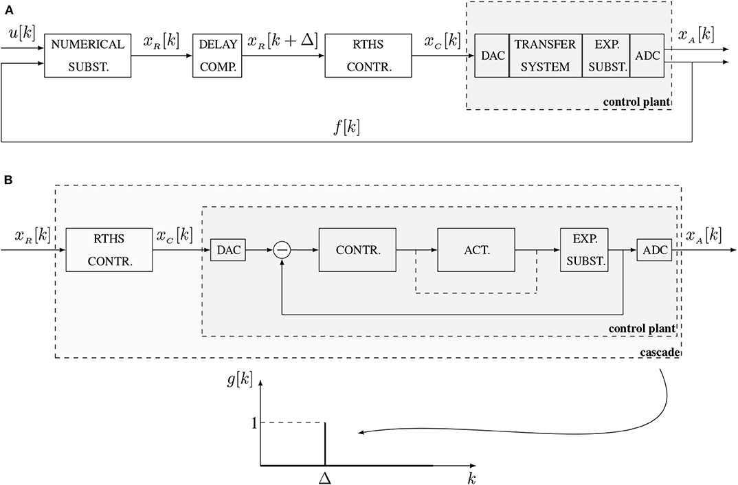
Figure 1. Layout of the RTHS framework. (A) The RTHS loop. (B) The cascade of the RTHS controller and the control plant, which ideally should compose a delayed unit impulse.

In more detail, it is assumed that an external excitation, u[k] is applied to the numerical substructure and the kinematics at the boundary are calculated by applying an appropriate numerical integration scheme that solves the equations of motion (Shing, 2008). The calculated reference signal, x_R[k], which can be in the form of displacement, velocity, or acceleration, is then applied though the transfer system to the experimental substructure. The response of the latter is monitored and the dynamics at the boundary, usually in the form of a force, is fed back as additional input to the numerical substructure, in order to proceed to the next step of the loop.

For the effective implementation of a RTHS loop, two fundamental problems must be solved. The first corresponds to the dynamics of the control plant and is treated by introducing an additional controller (termed the RTHS controller in Figure 1A). The second problem pertains to the delay that the transfer path inherits, which is tackled via an appropriate delay compensation method. Under this enriched configuration, the reference signal is predicted Δ steps forward, where Δ is an estimate of the transfer path's overall delay, and then appropriately modified via the RTHS controller to form the command signal for the transfer system. A careful tuning of all the individual blocks results in an achieved signal at the experimental substructure that is equal to the reference one, e.g., x_A[k] = x_R[k]; this equality forms the hard constraint of any RTHS loop. Under this setting, the challenge that this study aims to tackle is summarized in the following question: is it possible to tune a RTHS controller and a delay compensation algorithm without any prior information on the dynamics of the control plant, given only the availability of the reference and achieved signals?

Leaving out the delay problem for the moment, the data-driven attack to the establishment of a RTHS controller is illustrated in Figure 1B and reads as follows: under the availability of x_R[k] and x_A[k], a controller that forms the inverse of the control plant should be estimated, causing the cascade to perform as a perfect delay, e.g., x_A[k] = x_R[k − Δ]. Then, the addition of the delay compensation method should result in fulfilling the hard constraint condition of the RTHS loop. In designing such a controller, Dertimanis et al. (2015a) described a set of specifications, which are herein reformulated and enriched. According to these, a controller should be:

1. Data-driven: no need for analytical models of individual components (valves, cylinders, etc.) and identification of system parameters (stiffness, damping, oil constants, flow rates, etc.)

2. Feedforward-driven: no need for additional feedback loops.

3. Discrete-time oriented: no need for discretization of continuous-time models. Everything should be digital.

4. Minimally parametrized: the number of parameters, henceforth referred to as hyper-parameters, required for the proper tuning of the controller should be kept as small as possible. The controller should not be “too sensitive” on these hyper-parameters.

5. Of guaranteed stability: exclusive use of finite impulse response (FIR) models (refer to section 2.1), instead of infinite impulse response models in order to enforce stability and safety during test.

6. Robust: the RTHS controller should compensate for all uncertainties of the control plant, as well as the CSI problem.

7. Of minimum discrepancies: the cascade frequency response should follow the zero dB line in the maximum possible frequency band. The phase delay should be constant within this band.

8. Straightforward to implement to existing facilities: the RTHS controller should be opeational in conjunction with conventional fixed-gain controllers.

9. Applicable to a wide range of transfer systems: from small-scale actuators and light specimens, to shaking tables and specimens of several megagrams.

10. Functional for all types of command signals: both acceleration and displacement reference signals should be handled.

11. Straightforward to realize-execute: immediate implementation in commercial hardware and execution in real time. No need for sophisticated software design.

Our approach for establishing such an inverse controller utilizes the theory of adaptive signal processing (Widrow and Wallach, 2007; Diniz, 2008) and it can be implemented either online, or offline. Its effectiveness in modeling facilities for structural testing has already been demonstrated in Dertimanis et al. (2015a,b).

2.1. Brief Review of Adaptive Filtering

For convenience, this section offers a brief outline of the most fundamental concepts of adaptive signal processing. The familiarized reader can safely skip this summary. A sound treatment to the topic is given in Diniz (2008), Hayes (1996), and Manolakis et al. (2005). Glentis et al. (1999) provide an excellent review on adaptive filters, including the presentation of a comprehensive review of associated algorithms.

Consider an unknown plant that can be effectively described by its impulse response g[k] in the discrete-time domain, or by its transfer function G(z) in the ${Z}$-domain. The plant is driven by a wide-sense stationary input signal u[k] and the response x[k] is measured in a noise-corrupted fashion, under the assumption of an additive disturbance d[k] at the plant's output, which is random and uncorrelated to x[k]. Using an FIR parametrization, we can represent the input-output dynamics as

$\begin{array}{ll}x[k]={\displaystyle \sum _{i=0}^n}g[i]u[k-i]+d[k]& (1)\end{array}$

with n corresponding to the model order. For $\text{g}={[g[0]g[1]\dots g[n]]}^T\text{ and }\text{u}[k]={[u[k]u[k-1]\dots u[k-n]]}^T$ Equation (1) can be cast into a regression form

$\begin{array}{ll}x[k]={\text{u}}^T[k]\text{g}+d[k]& (2)\end{array}$

Suppose now that measurements of u[k] and x[k] are acquired and the aim is to estimate a FIR model of the plant. Our model reads

$\begin{array}{ll}\widehat{x}[k]={\displaystyle \sum _{i=0}^n}\widehat{g}[i]u[k-i]={\text{u}}^T[k]\widehat{\text{g}}& (3)\end{array}$

where $\widehat{x}[k]$ is the model's output and $\widehat{\text{g}}$ the vector of unknown filter weights. This is a typical parametric identification problem, which can be solved by collecting measurements over a time interval and then solving a linear least-squares problem for recovering g. Clearly, this non-recursive strategy cannot be applied in real-time, since it requires batch-processing of stored data.

An alternative approach is to proceed in a recursive estimation of the weights, whenever new data becomes available. The key idea, illustrated in Figure 2, is to update the weights via the stochastic approximation of a deterministic optimization algorithm, in which the direction is calculated using unbiased estimates on the basis of the current time index. For example, consider the steepest descent algorithm

$\begin{array}{ll}\widehat{\text{g}}[k+1]=\widehat{\text{g}}[k]-\mu \nabla V(\widehat{\text{g}}[k])& (4)\end{array}$

where μ is the step size and $V(\widehat{\text{g}}[k])$ is the objective function, defined as the instantaneous mean square error (MSE)

$\begin{array}{ll}V(\widehat{\text{g}}[k])=E\{e^2[k]\}=E\{{(\text{x}[k]-\widehat{\text{x}}[k])}^2\}& (5)\end{array}$

Plugging Equation (3) and differentiating with respect to $\widehat{\text{g}}[k]$ implies

$\begin{array}{ll}\nabla V(\widehat{\text{g}}[k])=-2E\{e[k]\text{u}[k]\}& (6)\end{array}$

Approximating the expectation operator E{e[k]u[k]} as e[k]u[k] and substituting to Equation (4) yields

$\begin{array}{ll}\widehat{\text{g}}[k+1]=\widehat{\text{g}}[k]+2\mu e[k]\text{u}[k]& (7)\end{array}$

This is the celebrated least mean square (LMS) adaptive filter developed by Widrow and Hoff (1960). Expectedly, the behavior of the algorithm depends on the step size. When d[k] is wide-sense stationary and the unknown plant is time-invariant, the LMS filter converges in the mean to the optimal Wiener solution, provided that μ is bounded as

$\begin{array}{ll}0<\mu <\frac{1}{{\lambda }_{\text{max}}}& (8)\end{array}$

where λ_max is the largest eigenvalue of the input's autocorrelation matrix

$\begin{array}{ll}{\Gamma }_{uu}=\left[\begin{array}{cccc}{\gamma }_{uu}[0]& {\gamma }_{uu}[1]& \dots & {\gamma }_{uu}[n]\\ {\gamma }_{uu}[1]& {\gamma }_{uu}[0]& \dots & {\gamma }_{uu}[n-1]\\ ⋮& ⋮& \ddots & ⋮\\ {\gamma }_{uu}[n]& {\gamma }_{uu}[n-1]& \dots & {\gamma }_{uu}[0]\end{array}\right]& (9)\end{array}$

for γ_uu[h] = E{u[k+h]u[k]}. The condition of Equation (8) does not, however, ensure stability. This is succeeded by

$\begin{array}{ll}0<\mu <\frac{1}{tr\{{\Gamma }_{uu}\}}=\frac{1}{(n+1){\sigma }_{uu}^2}& (10)\end{array}$

an expression that is widely used in practice, since it is based on the energy of the input signal, which is easier to calculate than the eigenvalues. Finally, maximum convergence speed is achieved when

$\begin{array}{ll}\mu =\frac{1}{{\lambda }_{\text{min}}+{\lambda }_{\text{max}}}& (11)\end{array}$

with λ_min denoting the smallest eigenvalue of Γ_uu. Equation (11) indicates that the speed is controlled by the eigenvalue spread of Γ_uu, e.g.,

$\begin{array}{ll}\text{eigenvalue spread}=\frac{{\lambda }_{\text{max}}}{{\lambda }_{\text{min}}}& (12)\end{array}$

From Equations (11, 12) it is easy to conclude that convergence speed requires an eigenvalue spread close to one. When the input signal can be selected by the user, the best option is to let u[k] being a realization of a zero-mean Gaussian white noise process, since ${\Gamma }_{uu}={\sigma }_{uu}^2{\text{I}}_{n+1}$ and the spread is equal to one.

FIGURE 2

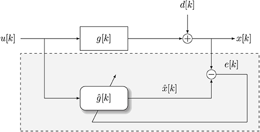
Figure 2. Sketch of the adaptive filtering concept for the system identification problem.

2.2. The Problem of Inverse Identification

Assume that the control plant can be described by the following digital rational transfer function

$\begin{array}{ll}G(z)=\frac{\theta (z)}{\varphi (z)}=\frac{{\theta }_0+{\theta }_1{z}^{-1}+{\theta }_2{z}^{-2}+\cdots +{\theta }_{n_{\theta }}{z}^{-n_{\theta }}}{1+{\varphi }_1{z}^{-1}+{\varphi }_2{z}^{-2}+\cdots +{\varphi }_{n_{\varphi }}{z}^{-n_{\varphi }}}& (13)\end{array}$

Then, the problem of identifying an inverse controller is reduced in approximating the inverse transfer function

$\begin{array}{ll}{G}^{-1}(z)=\frac{1+{\varphi }_1{z}^{-1}+{\varphi }_2{z}^{-2}+\cdots +{\varphi }_{n_{\varphi }}{z}^{-n_{\varphi }}}{{\theta }_0+{\theta }_1{z}^{-1}+{\theta }_2{z}^{-2}+\cdots +{\theta }_{n_{\theta }}{z}^{-n_{\theta }}}& (14)\end{array}$

If G(z) is strictly minimum phase (e.g., poles and zeros inside the unit circle), then the problem has a straightforward solution, since G⁻¹(z) will be also minimum phase, admitting a convergent expansion of the form

$\begin{array}{ll}{G}^{-1}(z)={\displaystyle \sum _{i=0}^{\infty }}{g}_I[i]z^{-i}& (15)\end{array}$

with g_I[0] = 1 and

$\begin{array}{ll}{\displaystyle \sum _{i=0}^{\infty }}\left|g_I[i]\right|<\infty & (16)\end{array}$

Thus, by truncating the infinite sum up to an order n_I, it is possible to derive a FIR representation for the inverse controller. If, however, G(z) is non-minimum phase, the poles of G⁻¹(z) [e.g., the zeros of G(z)] are located outside the unit circle and the power expansion of Equation (15) diverges. To cope with this issue, recall that a digital transfer function admits two inverse ${Z}$-transforms, a causal and a non-causal one, depending on the region of convergence (Oppenheim et al., 1999, Chapter 3). In the case of the non-minimum phase G(z), the causal inverse transform is unstable, but the non-causal is stable. A stable, non-causal expansion of G⁻¹(z) can be written as

$\begin{array}{ll}{G}^{-1}(z)={\displaystyle \sum _{i=0}^{n_1}}{g}_I[i]z^{-i}+{\displaystyle \sum _{\ell =0}^{\infty }}{g}_I[\ell ]z^{\ell }& (17)\end{array}$

where, usually, the causal part is limited to very few terms (e.g., n₁ is small). If the weights of the non-causal part are significant, attempting to adapt an inverse controller would render quite poor results. However, if one would consider multiplying Equation (17) by a pure delay, z ^{− Δ}, it would cause Δ weights to jump from the non-causal to the causal part, increasing thus the accuracy of the inverse (Widrow and Wallach, 2007, Chapter 5).

To summarize, the adaptation of the inverse controller aims at satisfying the following equation

$\begin{array}{ll}{z}^{-\Delta }{G}^{-1}(z)G(z)\to 1& (18)\end{array}$

In practice, this implies that the reference signal passes through a pure delay before being fed to the adaptation block. It is emphasized that, even if the continuous-time transfer function of a plant is minimum phase, its digital counterpart may oftentimes result non-minimum phase.

3. Adaptive Inverse Control for RTHS

3.1. Description

The control strategy implemented herein essentially pertains to applying the adaptive filtering concepts previously outlined in identifying an appropriate inverse controller. The latter is then placed before the plant in the signal path, such that the cascade results ideally in a delayed unit impulse response. Accordingly, by integrating an appropriate delay compensation method, the achieved signal may follow the reference one with a reasonable accuracy, at a certain frequency band.

The strategy used for the adaptation of this inverse controller is based on the simple architecture shown at Figure 3 and consists of two stages that are implemented in (hard) real-time:

- The forward adaptation stage, where an FIR estimate of g[k], $\widehat{g}$_F[k], is obtained.

- The inverse adaptation stage, where an FIR estimate of the inverse of g[k], $\widehat{g}$_I[k], is obtained, making use of $\widehat{g}$_F[k].

FIGURE 3

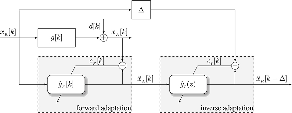
Figure 3. The learning process of the adaptive inverse controller.

These two phases can either be performed successively or simultaneously, in the sense that it is not necessary to wait for the full convergence of the forward controller, in order to start the adaptation of the inverse one (Widrow and Wallach, 2007).

The adaptation process initiates by supplying a reference signal, x_R[k], of favorable properties (see below), to the control plant. This signal, together with the noise-corrupted achieved response of the plant, x_A[k] are fed to the forward adaptation block, for estimating a FIR filter that describes the end-to-end reference-achieved signal dynamics. The term end-to-end herein implies that the path from the reference to the achieved signal contains all individual software/hardware components, including ADCs, DACs, signal conditioners, etc., besides the control plant.

When the forward and inverse adaptation are carried out simultaneously, e.g., in synchronous mode, the instantaneous estimate of the achieved response, ${\widehat{x}}_A[k]$, together with a delayed version of the original reference signal, are fed to the inverse adaptation block and a FIR filter is tuned for describing the achieved-(delayed) reference signal dynamics. The output of this block is an estimate of x_R[k − Δ] (see Figure 3). The delay Δ is an algorithmic parameter (it is included in the set of method's hyper-parameters, listed in Table 1) and its size depends heavily on the qualitative characteristics of the control plant.

TABLE 1

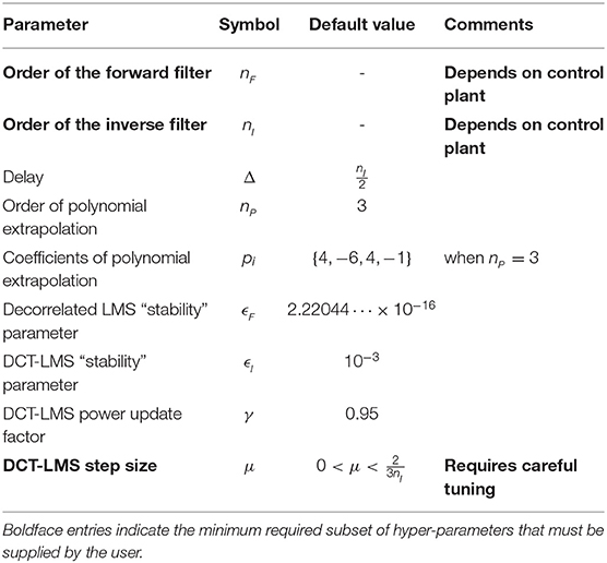
Table 1. Method's hyper-parameters.

A key detail of the presented algorithm is that the inverse filter weights are not adapted by directly feeding the output of the control plant to the inverse block, in order to avoid the propagation of the disturbance. When both stages have been successfully executed and convergence has been achieved, the inverse FIR filter can be copied before the control plant and it is implemented as an inverse controller. Ideally, the cascade of the inverse controller and the control plant form a unit impulse that reproduces a delayed version of any reference signal. It is noted that more sophisticated algorithms can be implemented as adaptive inverse controllers, as the modified filtered-X one presented in the work of Dertimanis et al. (2015a).

3.2. Forward Adaptation

Our choice for the algorithm that implements the forward adaptation path is based on (i) the reported convergence rates; and (ii) the reduction of the required tuning parameters. Based on previous results (Dertimanis et al., 2015a,b) we apply the decorrelated LMS algorithm Doherty and Porayath (1997), which belong to the class of instrumental variable methods (Glentis et al., 1999). At each step, the adaptive filter's output is calculated as

$\begin{array}{ll}{\widehat{x}}_A[k]={\text{x}}_R^T[k]{\text{g}}_F[k]& (19)\end{array}$

where

$\begin{array}{ll}{\begin{array}{l}{\text{x}}_R[k]=\left[x_R[k]x_R[k-1]\dots x_R[k-n_F]\right]\hfill \end{array}}^T& (20)\end{array}$

$\begin{array}{ll}{\begin{array}{l}{\widehat{\text{g}}}_F^T[k]=\left[{\widehat{g}}_F[k,0]{\widehat{g}}_F[k,1]\dots {\widehat{g}}_F[k,n_F]\right]\hfill \end{array}}^T& (21)\end{array}$

and n_F is the order of the filter. The coefficients are updated by

$\begin{array}{ll}{\widehat{g}}_F[k+1]={\widehat{g}}_F[k]+\mu [k]\text{w}[k]& (22)\end{array}$

for a step size μ[k]

$\begin{array}{ll}\mu [k]=\frac{e_F[k]}{{\text{x}}_R^T[k]\text{w}[k]+{ϵ}_F}& (23)\end{array}$

In Equation (23), ϵ_F is a small constant (“stability” parameter), $e_F[k]=x_A[k]-{\widehat{x}}_A[k]$ is the error between the measured and the predicted signal and w[k] is the filter gradient, updated by

$\begin{array}{ll}\text{w}[k]={\text{x}}_R[k]-\alpha [k]{\text{x}}_R[k-1]& (24)\end{array}$

with a[k] denoting the decorrelation coefficient

$\begin{array}{ll}a[k]=\frac{{\text{x}}_R^T[k]{\text{x}}_R[k-1]}{{\text{x}}_R^T[k-1]{\text{x}}_R[k-1]}& (25)\end{array}$

The properties of the decorrelated LMS algorithm are studied in Doherty and Porayath (1997). See also (Douglas et al., 1999; Rørtveit and Husøy, 2009). As an alternative to the decorrelated LMS, the normalized LMS algorithm (Diniz, 2008, Chapter 4) can be also applied to the forward adaptation path, at the cost of an additional hyper-parameter that controls the adaptation step.

3.3. Inverse Adaptation

The signal that arrives at the input of the inverse adaptation block, ${\widehat{x}}_A[k]$ is, in general, highly correlated (e.g., colored), since it describes the dynamics of the control plant. Notice that when the reference signal is Gaussian-like, the inverse adaptation pertains essentially to a whitening process. This is because, the cascade of the inverse controller and the plant should give an achieved signal which is uncorrelated like the Gaussian input. As the convergence rate of the conventional LMS algorithm (including its normalized version) is adversely affected by correlated inputs, it cannot be considered as a competitive candidate. Instead, an effective solution to this problem is offered by transform domain methods, which utilize an orthogonal transformation to a space that is attributed with favorable properties (Beaufays, 1995; Diniz, 2008; Chergui and Bouguezel, 2017).

Setting temporarily ${\widehat{x}}_R[k-\Delta ]=y[k]$ for notational convenience (see Figure 3), the output of the inverse filter reads

$\begin{array}{ll}y[k]={\displaystyle \sum _{i=0}^{n_I}}{\widehat{g}}_I[k,i]{\widehat{x}}_A[k-i]={\widehat{\text{x}}}_A^T[k]{\widehat{\text{g}}}_I[k]& (26)\end{array}$

For any orthogonal matrix $\text{S}\in {ℝ}^{n_I}$, the regression form of Equation (26) can be written as

$\begin{array}{ll}y[k]={\widehat{\text{x}}}_A^T[k]{\text{S}}^T\text{S}{\widehat{\text{g}}}_I[k]={\text{u}}^T[k]\text{c}[k]& (27)\end{array}$

for $\text{u}[k]=\text{S}{\widehat{\text{x}}}_A[k]$ and $\text{c}[k]=\text{S}{\widehat{\text{g}}}_I[k]$. The orthogonal transformation of the input can be considered as another type of decorrelation. However, it has small effects on the convergence rate. The latter is treated by normalizing the entries of the transformed input vector by the square root of their power via

$\begin{array}{ll}{v}_i[k]=\frac{1}{\sqrt{P_i[k]+{ϵ}_I}}{u}_i[k],i=0,1,\dots ,n_I& (28)\end{array}$

where ϵ_I is a small constant (“stability” parameter),

$\begin{array}{ll}{P}_i[k]=\gamma P_i[k-1]+(1-\gamma )u_i^2[k],i=0,1,\dots ,n_I& (29)\end{array}$

and γ → 1 is the power update factor. The transformed weights are then updated by a typical LMS filtering operation

$\begin{array}{ll}\text{c}[k+1]=\text{c}[k]+\mu e[k]\text{v}[k]& (30)\end{array}$

with μ being the step size, $e_I[k]=x_R[k-\Delta ]-y[k]=x_R[k-\Delta ]-{\widehat{x}}_R[k-\Delta ]$ the inverse adaptation error and $v[k]={[v_1[k]\dots v_{n_I}[k]]}^T$.

There's a plenty of options for the selection of the orthogonal matrix S, including the discrete Fourier transform (DFT), the discrete Hartley transform (DHT) and the discrete cosine transform (DCT). Herein, we adopt the third option and we construct the orthogonal matrix as

$\begin{array}{ll}\text{S}=\left[\begin{array}{cccc}{Q}_{0,0}& Q_{0,1}& \dots & Q_{0,n_I-1}\\ Q_{1,0}& Q_{1,1}& \dots & Q_{1,n_I-1}\\ ⋮& ⋮& \ddots & ⋮\\ Q_{n_I-1,0}& Q_{n_I-1,1}& \dots & Q_{n_I-1,n_I-1}\end{array}\right]& (31)\end{array}$

where

$\begin{array}{ll}{Q}_{p,q}=\sqrt{\frac{2}{n_I}}{K}_p\text{cos}(\frac{p(q+1/2)\pi }{n_I}),p,q=0,1,\dots ,n_I-1& (32)\end{array}$

for

$\begin{array}{ll}{K}_p=\{\begin{array}{cc}\frac{1}{\sqrt{2}},& p=0\\ 1,& p\ne 0\end{array}& (33)\end{array}$

Since the DCT transform is fully parametrized by the filter order, the orthogonal matrix S can be formulated and stored prior to the adaptive modeling process. Further details on the performance of transform domain adaptive algorithms can be found in Zhao et al. (2009), Kim and Wilde (2000), Lee and Un (1986), and Narayan et al. (1983).

3.4. Delay Compensation and Method's Hyper-Parameters

The successful adaptive modeling of the control plant and its inverse forces, ideally, the cascade to behave as a delayed unit impulse. This implies that a reference signal is driven to the control plant with unaltered dynamics, but at a delay Δ. To compensate for this delay, we integrate a one-step ahead prediction method, which is based on polynomial extrapolation (Horiuchi et al., 1999; Darby et al., 2001; Wallace et al., 2005). The reference signal that is driven to the inverse controller is

$\begin{array}{ll}{x}_R[k+\Delta ]={\displaystyle \sum _{i=0}^{n_P}}{p}_i{x}_R[k-i\Delta ]& (34)\end{array}$

where n_P is the polynomial order and p_i the polynomial coefficients, which are calculated via the Lagrange basis function and are predefined for a given order.

Table 1 gathers all the hyper-parameters of the method. The most important of them pertain to the orders of the forward and the inverse adaptive filters, as well as to the step size of the DCT-LMS: these are essentially the quantities that the user has to decide for, every time a new experimental substructure is attached to a transfer system, composing thus the control plant. The default order of the polynomial extrapolation is sufficient, as long as the cascade is close to a pure delay. Higher orders do not, in general improve accuracy; actually they might oftentimes lead to instability, especially when Δ is large.

4. Application Study

4.1. The vRTHS Benchmark Structure

In evaluating the performance of novel control schemes for RTHS in a safe manner, vRTHS offers a useful platform. VRTHS involves the implementation of a hybrid simulation fully in silico, whereby both the numerical substructure and the physical substructure are simulated. Crucially, vRTHS also involves recreation of the transfer functions associated with the actuation and signal artifacts associated to the actual physical implementation. The use of vRTHS can allow for rapid and safe assessment of various algorithms relating to the hybrid simulation procedure. The robustness of any algorithm can also be investigated by the introduction of uncertainty in the vRTHS.

The study of suitable control and delay compensation algorithms for RTHS has resulted in proposition of alternatives schemes, which have been investigated on disparate testing setups. However, hybrid simulation setups tend to be unique and hence it is difficult to fairly evaluate the relative performance of control schemes implemented on different setups. This provides the motivation for establishing benchmark problems, wherein the only variable is the control regime implemented.

Such a benchmark problem is recently proposed by Silva et al. (2020), who developed a vRTHS framework for the purpose of evaluating different control regimes on a unified system. This benchmark consists of a 2-bay, 3-story steel frame, in which the structural mass is concentrated on the floors, motion is allowed only horizontally on a single direction and damping is proportional. An originally 30-degrees of freedom (DOFs) linear elastic planar finite element model is reduced to a 3-DOF model, pinned at ground and excited on its base, which consists the reference structure (Figure 4). The benchmark is implemented in SIMULINK^© and is created such that the controller block can easily be exchanged, whilst the rest of the system is left unchanged. This allows for the fair comparison of controllers. A number of uncertainties in the system parameters is also offered, to allow for analysis of controller robustness, along with a set of standardized performance metrics to aid comparison.

FIGURE 4

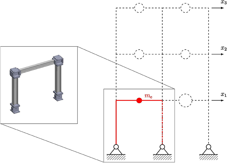
Figure 4. The reduced 3-DOF benchmark frame and its partitioning into an experimental and a numerical substructure. Reproduced from Silva et al. (2020) with permission from Elsevier.

For the vRTHS tests the reference structure is partitioned into an “experimental” and a numerical substructure, with the former corresponding to a single bay of the ground floor and the latter consisting of the remainder of the structure (Figure 4). The structural properties of the experimental substructure are kept fixed, while the ones of the numerical substructure vary in accordance to the partition schemes of Table 2.

TABLE 2

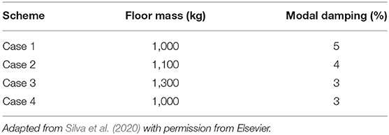
Table 2. vRTHS partitioning cases.

The dynamics of the control plant (transfer system plus experimental substructure) are described as shown in Figure 5. The open-loop transfer function between the command and the achieved signals in continuous-time reads

$\begin{array}{ll}G(s)=\frac{B_0}{A_5{s}^5+A_4{s}^4+A_3{s}^3+A_2{s}^2+A_{1}s+A_0}& (35)\end{array}$

for

$\begin{array}{l}{B}_0={\alpha }_1{\beta }_0{A}_0=k_e{\alpha }_3{\beta }_2+{\alpha }_1{\beta }_0\\ A_1=k_e{\alpha }_3{\beta }_1+(k_e+c_3{\alpha }_3+{\alpha }_2){\beta }_2\\ A_2=k_e{\alpha }_3+(k_e+c_3{\alpha }_3+{\alpha }_2){\beta }_1+(c_e+m_e{\alpha }_3){\beta }_2\\ A_3=(k_e+c_3{\alpha }_3+{\alpha }_2)+(c_e+m_e{\alpha }_3){\beta }_1+m_e{\beta }_2\\ A_4=c_e+m_e{\alpha }_3+m_e{\beta }_1\end{array}$

$\begin{array}{ll}{A}_5=m_e& (36)\end{array}$

The numerical values of all associated parameters are listed in Table 3. To incorporate a degree of uncertainty, for testing the robustness of a proposed controller, some parameters are defined as normally distributed random variables.

FIGURE 5

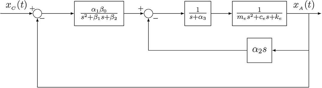
Figure 5. Layout of the control plant. From left to right, the transfer functions on the upper branch correspond to the valve, actuator and experimental substructure dynamics, respectively, while the transfer function on the inner feedback loop corresponds to the control-structure interaction dynamics. Adapted from Silva et al. (2020) with permission from Elsevier.

TABLE 3

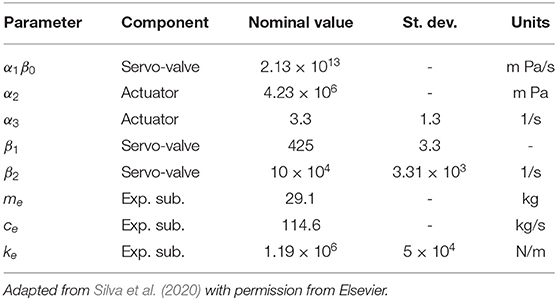
Table 3. Parameter values for the control plant of Figure 5.

All vRTHS tests are conducted in SIMULINK^© through the integration of the structural equations of motion via an explicit 4th-order Runge-Kutta numerical framework, at a fixed sampling rate F_s = 4, 096 Hz. It is emphasized that the choice of the integration scheme has detrimental effects on the evolution of the dynamics and, consequently, on the behavior on the proposed adaptive modeling method. To demonstrate this, Figure 6 displays the discrete-time impulse response of the control plant under two different discretization schemes: in the upper plot, g[k] is calculated via the aforementioned integration, by applying a unit impulse excitation to the part of the SIMULINK^© model that corresponds to Figure 5. In the lower part, the impulse response is obtained by the impulse-invariance transformation of Equation (35), e.g., g[k] = T_sg(t = kT_s), where g(t) is the continuous-time impulse response (the inverse Laplace transform of Equation 35). A quite different “damped” behavior is observed, which renders the integration-based impulse response attaining a much slower decay rate, necessitating the use of very high order FIR models for effective adaptive modeling of the control plant.

FIGURE 6

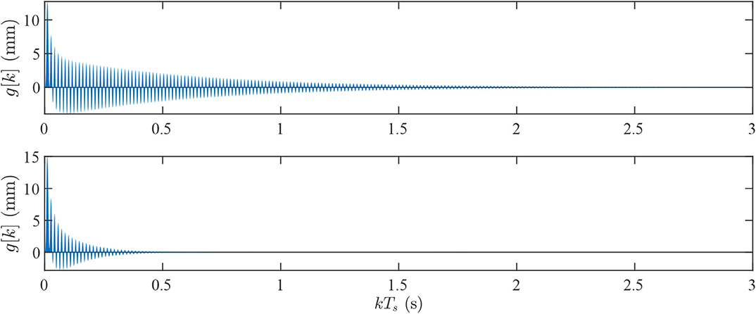
Figure 6. Control plant's impulse response. Upper: 4th-order Runge-Kutta integration. Lower: zero-order hold discretization of Equation (35). Rate fixed in both cases at F_s = 4096 Hz.

4.2. Adaptive Modeling

For generating the reference signal, a Markov-1 process of the form

$\begin{array}{ll}u[k]+{\varphi }_{1}u[k-1]=e[k]& (37)\end{array}$

is adopted, where e[k] is a zero-mean Gaussian white noise stochastic process of variance ${\sigma }_{ee}^2$. In deciding for the values of ϕ₁ and ${\sigma }_{ee}^2$, recall that the maximum and minimum eigenvalues of Γ_uu are provided by the corresponding maximum and minimum of the power spectrum of u[k], which is given by

$\begin{array}{ll}{S}_{uu}(f)=\frac{1}{1+2\text{ cos}(2\pi \frac{f}{F_s}){\varphi }_1+{\varphi }_1^2}{\sigma }_{ee}^2& (38)\end{array}$

Thus,

$\begin{array}{l}{\lambda }_{\text{max}}={(1-{\varphi }_1)}^2{\sigma }_{ee}^2\\ {\lambda }_{\text{min}}={(1+{\varphi }_1)}^2{\sigma }_{ee}^2\end{array}$

and the eigenvalue spread for Γ_uu is

$\begin{array}{ll}\text{eigenvalue spread}=(\frac{1-{\varphi }_1}{1+{\varphi }_1}{)}^2& (39)\end{array}$

In order to maintain this number close to one, our choice is ϕ₁ = −0.01 (the minus sign is adopted for attributing S_uu(f) with low pass characteristics). The variance of e[k] is then determined by first setting 2σ_uu = 0.01, for constraining 95% of the input's amplitude within the ±10 mm range. From the theoretical Markov-1 process variance

$\begin{array}{ll}{\sigma }_{uu}^2=\frac{1}{1-{\varphi }_1^2}{\sigma }_{ee}^2& (40)\end{array}$

solving for ${\sigma }_{ee}^2$ leads to ${\sigma }_{ee}^2\approx 2.5\times 10^{-5}$.

The adaptation process is carried out simultaneously, that is, the forward and the inverse adaptation counterparts operate in synchronous mode. Having established the statistics of the reference signal, several trials are performed for the rest of the hyper-parameters of the method (e.g., the forward and inverse filter orders and the step size of the DCT-LMS), while the total adaptation time frame is fixed to 60 s. Some critical observations during the evolution of the whole adaptation process can be summarized by the following remarks:

- In all trials the convergence in synchronous mode is quite fast and robust against the DCT-LMS step size. The forward adaptation phase requires at least around 10–15 s for proper convergence.

- Within this time the DCT-LMS makes a rapid improvement, indicating that full convergence of the forward filter is not necessary for adapting the inverse.

- A proper selection of the DCT-LMS step size is important. In many cases, a quite fast convergence is observed, yet, the final result is not optimal in terms of cascade dynamics, as the corresponding impulse response returns “noisy.”

- It is noted that a fair number of trials is conducted by applying non-Markovian inputs, as well as other adaptive algorithms. Regarding the former, signals composed from filtering Gaussian white noise at cut-off frequencies equal to 100 Hz and F_s/2 are also tested. The result is a severe distortion in the filters' weights, followed by inability to converge within the specified time frame. Very slow convergence is also observed in the case where the normalized LMS algorithm replaces the DCT-LMS one for the adaptation of the inverse filter. This is, though, an expected result, attributed to the inability of the algorithm to cope with colored inputs.

Aspects of these remarks can be visually validated from Figures 7–10, which display the results for n_F = 10, 000 and n_I = 100 (Δ = 50, μ = 5 × 10⁻³), our final choice for the forward and inverse FIR filters. The fact that $\widehat{g}$_F[k] is very long (Figure 7, top) is explained by the high sampling rate of the simulation (4,096 Hz): in absolute times this impulse response evolves over 2.14 s (the settling time of the control plant's step response is around 1 s). It is noted that when lower orders are considered (for example 8,000 and 9,000 weights), an apparent distortion around the last weights of the cascade is caused: in fact, this is a practical way of detecting that the forward filter requires higher orders. The absolute error (Figure 8, upper part) confirms that convergence has been succeeded already after 15–20 s.

FIGURE 7

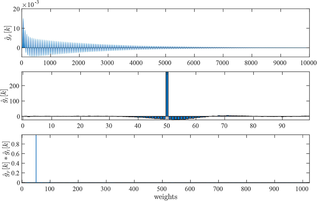
Figure 7. Estimated forward (Top) and inverse (Middle) adaptive filters, and their cascade (Bottom).

FIGURE 8

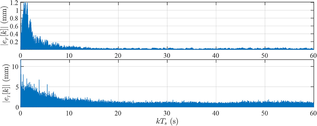
Figure 8. Forward (Top) and inverse (Bottom) absolute adaptation errors for the filters of Figure 7.

FIGURE 9

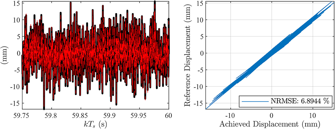
Figure 9. Left: delayed reference (continuous black line) and achieved (dashed red line) signals during the last 0.25 s of the adaptation process. Right: synchronization plot of the signals on the left. NRMS, normalized root means square error (Figure 7).

FIGURE 10

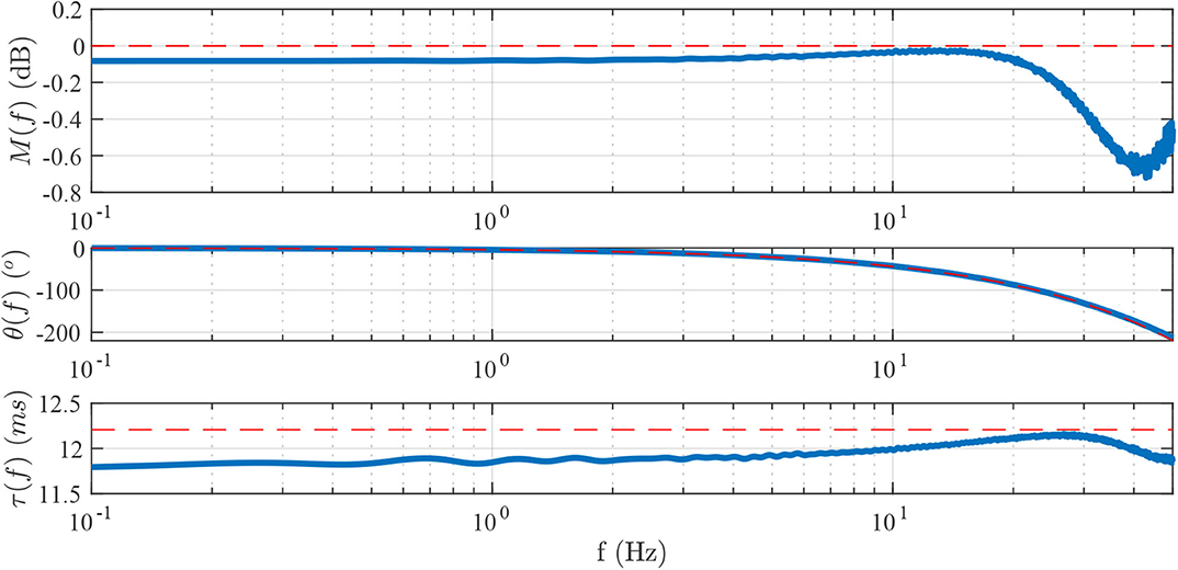
Figure 10. Frequency response of the cascade in the [0.1, 100] Hz band (Top: amplitude, Middle: phase), and associated phase delay (Bottom). The dashed red lines correspond to the frequency response and phase delay of the perfect digital impulse response with Δ = 50.

In contrast, the inverse filter dynamics are expanded in a considerably smaller time frame (around 24 ms, Figure 7, middle). The dominant part of $\widehat{g}$_I[k] is located around the chosen delay (which is typical for inverse filters) and there exist many leading and trailing weights that could, potentially, be treated as zeros. However, adaptation at lower order/delay pairs (indicatively 80/40, 60/30, and 40/20), or at fixed order (n_I = 100) and lower delays (e.g., Δ = 40, 30, and20) does not improve the inverse controller. Thus, the 100/50 pair results as the lowest possible accurate choice for this plant.

The absolute adaptation error (Figure 8, bottom) exhibits fast convergence (after approximately 25-30 s), with longer time needed however for a finer tuning of the weights; it is observed that by reducing the adaptation time to half the fixed frame (e.g., 30 s) and keeping all other hyper-parameters unaltered leads to sub-par results. It is also worth mentioning that the converged values for |e_I[k]| are higher in comparison to the ones of |e_F[k]|. This is also expected since, as already mentioned in section 3.3, the inverse adaptation performs as a whitening filter. Indicatively, Figure 9 shows the synchronization plot between the delayed reference and the achieved signals for the last 0.25 s of the adaptation process. A normalized root-mean-square error, defined as

$\begin{array}{ll}\text{NRMSE}=\sqrt{\frac{{\displaystyle {\sum }_{k=1}^N}{(x_R[k]-{\widehat{x}}_R[k])}^2}{{\displaystyle {\sum }_{k=1}^N}{x}_R^2[k]}}& (41)\end{array}$

of approximately 7% is estimated.

The cascade of $\widehat{g}$_F[k] and $\widehat{g}$_I[k], the first 1,024 weights of which are plotted in Figure 7, bottom, depicts a very good approximation to a pure delay. This is verified in the frequency domain against the perfect digital impulse with Δ = 50; as Figure 10 displays, there is a quite close resemblance between the frequency responses and the associated phase delays between the estimated and the perfect delayed impulses. The highest distortion in amplitude, located around 40 Hz, is not more than −0.8 dB, whereas the largest difference in phase delay is approximately 0.5 ms.

In order to obtain a better insight on the effects of the observed distortions in the frequency domain, a number of open loop simulations is conducted with the adaptive inverse controller placed before the control plant. Different signals are selected as references, including sinusoids at different frequencies, a chirp, low pass filtered Gaussian white noise, as well as the structural response of DOF x₁ for the El Centro earthquake (40% scaling). The results of the simulations are again interpreted in terms of synchronization plots and are shown in Figure 11. Apart from the case of 40 Hz (Figure 11C), which returns a NRMSE value of approximately 8%, all other simulations produce achieved signals of good quality in a wide frequency range.

FIGURE 11

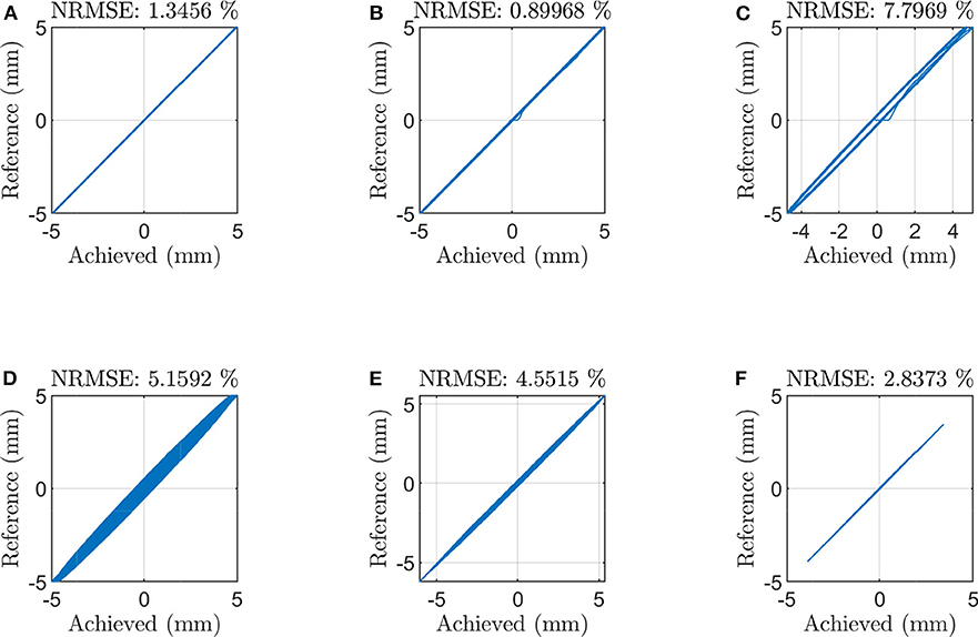
Figure 11. Synchronization plots between the delayed reference (Δ = 50) and achieved signals during open loop adaptive inverse control simulations. (A) sinusoid at 1 Hz, (B) sinusoid at 20 Hz, (C) sinusoid at 40 Hz, (D) chirp with linear frequency increase between [0, 10] Hz, (E) zero-mean Gaussian white noise low pass filtered at 15 Hz, and (F) structural response of DOF x₁ for the El Centro earthquake (40% scaling).

4.3. vRTHS

We are now almost ready to integrate the estimated adaptive inverse controller to the vRTHS closed loop. To this end, the delay compensation scheme outlined in section 3.4 is applied and the reference signal that is sent to the adaptive inverse controller is calculated from Equation (34) as

$\begin{array}{ll}{x}_r[k+\Delta ]=4x_1[k]-6x_1[k-\Delta ]+4x_1[k-2\Delta ]-x_1[k-3\Delta ]& (42)\end{array}$

where x₁[k] is the displacement of the interface DOF calculated at time k and Δ = 50, which corresponds to a cascade delay of 12.2 ms. The numerical substructure is excited by the El Centro earthquake at 40% intensity, while for each case of Table 2 20 individual simulations are executed. The results are presented in terms of the criteria J₁ to J₉ that are reported in Silva et al. (2020) and listed in Table 4.

TABLE 4

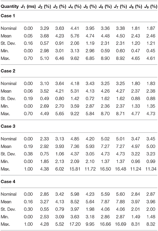
Table 4. vRTHS evaluation criteria for the partitioning cases of Table 2.

The following points summarize the performance of the proposed data-driven method:

- The delay between the reference and the achieved displacement (e.g., J₁) is exactly zero in all nominal simulations, and very low in the perturbed simulations of all partitioning case studies. The statistics of the perturbed simulations are comparable, indicating robustness of the controller against uncertainty. It is noted that the total number of non-zero delay simulations are 3, 2, 5 and 5 in partitioning case studies 1 to 4, respectively. This is illustrated in Supplementary Tables 1–4.

- The NRMSE between the reference and the achieved displacement (e.g., J₂) is also kept quite low, ranging from 2.85 to 3.29% in the nominal simulations. These numbers are within the range of the NRMSEs shown at the synchronization plots of Figure 11. The mean values of the perturbed simulations follow closely the ones of their nominal counterparts, whereas the corresponding standard deviations are one order of magnitude lower.

- Expectedly, the normalized peak tracking error (e.g., J₃) returns a bit increased, compared to J₂, but again is kept in very low levels.

- Criteria J₄ to J₆ calculate the NRMSEs between the relative displacements of the storys during vRTHSs and the ones during the simulation of the reference structure (e.g., without substructuring), while J₇ to J₉ the normalized peak tracking errors of the same quantities. The associated errors never exceed 6% in the nominal cases, whereas the mean values of the perturbed simulations are higher (reaching up to 8.52% in partitioning case study 4), followed by increased dispersions. It is, however, noted that in the offered benchmark problem, the simulation of the reference structure is accomplished via a different discretization scheme (either zero, or first order hold), to the one implemented for vRTHS (e.g., the explicit 4th-order Runge-Kutta integration) and, as shown in Figure 6 there might be significant differences in the calculated structural responses.

We conclude that the efficacy and robustness of the adaptive inverse controller is quite competitive in all partitioning case studies. In comparing the method presented herein, the reader may refer to Silva et al. (2020), Wang et al. (2019), Najafi and Spencer (2019), Fermandois (2019), and Ning et al. (2019), where several alternative approaches for RTHS are developed and assessed through the same vRTHT benchmark problem.

5. Conclusions

In this study, we explore the possibility of conducting RTHS from a purely data-driven perspective. By setting a number of specifications that such a framework should fulfill, we demonstrate that this is indeed feasible and it is characterized by several potential advantages, including transparency, robustness and minimum tuning. Further improvements are possible, such as a more rigorous methodology for automating/adapting the selection of the method's hyper-parameters to the examined case study, the integration of the delay compensation to the adaptation process, as well as techniques for reducing the delay of the cascade's impulse and increasing the effective frequency band of RTHS. These are left as objectives of future work together with the design and conduction of an extensive experimental campaign for the validation of the method.

Data Availability Statement

The software and data developed for this study are available upon request to the corresponding author.

Author Contributions

TS: methodology, conduction of simulations, and manuscript preparation. VD: conceptualization, methodology, conduction of simulations, and manuscript preparation. EC: methodology, supervision, manuscript preparation, and funding acquisition.

Funding

This work was carried out as part of the ITN project DyVirt and has received funding from the European Union's Horizon 2020 research and innovation programme under the Marie Skłodowska-Curie grant agreement no. 764547.

Conflict of Interest

The authors declare that the research was conducted in the absence of any commercial or financial relationships that could be construed as a potential conflict of interest.

Supplementary Material

The Supplementary Material for this article can be found online at: https://www.frontiersin.org/articles/10.3389/fbuil.2020.570947/full#supplementary-material

References

Bayer, V., Dorka, U. E., Füllekrug, U., and Gschwilm, J. (2005). On real-time pseudo-dynamic sub-structure testing: algorithm, numerical and experimental results. Aerospace Sci. Technol. 9, 223–232. doi: 10.1016/j.ast.2005.01.009

CrossRef Full Text | Google Scholar

Beaufays, F. (1995). Transform-domain adaptive filters: an analytical approach. IEEE Trans. Signal Process. 43, 422–431. doi: 10.1109/78.348125

CrossRef Full Text | Google Scholar

Benson Shing, P. (2008). “Real-time hybrid testing techniques,” in Modern Testing Techniques for Structural Systems, eds O. S. Bursi and D. Wagg (Vienna: Springer), 259–292. doi: 10.1007/978-3-211-09445-7_6

CrossRef Full Text | Google Scholar

Carrion, J. E., and B. F. Spencer, J. (2006). “Real-time hybrid testing using model-based delay compensation,” in 4th International Conference on Earthquake Engineering (Taipei), 299.

Google Scholar

Chae, Y., Kazemibidokhti, K., and Ricles, J. M. (2013). Adaptive time series compensator for delay compensation of servo-hydraulic actuator systems for real-time hybrid simulation. Earthquake Eng. Struct. Dyn. 42, 1697–1715. doi: 10.1002/eqe.2294

CrossRef Full Text | Google Scholar

Chen, C., and Ricles, J. M. (2009). Improving the inverse compensation method for real-time hybrid simulation through a dual compensation scheme. Earthquake Eng. Struct. Dyn. 38, 1237–1255. doi: 10.1002/eqe.904

CrossRef Full Text | Google Scholar

Chergui, L., and Bouguezel, S. (2017). A new pre-whitening transform domain LMS algorithm and its application to speech denoising. Signal Process. 130, 118–128. doi: 10.1016/j.sigpro.2016.06.021

CrossRef Full Text | Google Scholar

Darby, A. P., Blakeborough, A., and Williams, M. S. (2001). Improved control algorithm for real-time substructure testing. Earthquake Eng. Struct. Dyn. 30, 446–448. doi: 10.1002/eqe.18

CrossRef Full Text | Google Scholar

Dertimanis, V., Mouzakis, H., and Psycharis, I. (2015a). On the acceleration-based adaptive inverse control of shaking tables. Earthquake Eng. Struct. Dyn. 44, 1329–1350. doi: 10.1002/eqe.2518

CrossRef Full Text | Google Scholar

Dertimanis, V., Mouzakis, H., and Psycharis, I. (2015b). “On the control of shaking tables in acceleration mode: an adaptive signal processing framework,” in Experimental Research in Earthquake Engineering: EU-SERIES Concluding Workshop, eds F. Taucer and R. Apostolska (Cham: Springer International Publishing), 159–172. doi: 10.1007/978-3-319-10136-1_12

CrossRef Full Text | Google Scholar

Diniz, P. S. R. (2008). Adaptive Filtering: Algorithms and Practical Implementation, 3rd Edn. New York, NY: Springer.

Google Scholar

Doherty, J., and Porayath, R. (1997). A robust echo canceler for acoustic environments. IEEE Trans. Circ. Syst. II Anal. Digit. Signal Process. 44, 389–396. doi: 10.1109/82.580846

CrossRef Full Text | Google Scholar

Douglas, S. C., Cichocki, A., and Amari, S. (1999). Self-whitening algorithms for adaptive equalization and deconvolution. IEEE Trans. Signal Process. 47, 1161–1165. doi: 10.1109/78.752617

CrossRef Full Text | Google Scholar

Fermandois, G. A. (2019). Application of model-based compensation methods to real-time hybrid simulation benchmark. Mech. Syst. Signal Process. 131, 394–416. doi: 10.1016/j.ymssp.2019.05.041

CrossRef Full Text | Google Scholar

Glentis, G.-O., Berberidis, K., and Theodoridis, S. (1999). Efficient least squares adaptive algorithms for fir transversal filtering. IEEE Signal Process. Mag. 16, 13–41. doi: 10.1109/79.774932

CrossRef Full Text | Google Scholar

Hayes, M. H. (1996). Statistical Digital Signal Processing and Modeling. New York, NY: John Wiley & Sons Ltd.

Horiuchi, T., Inoue, M., Konno, T., and Namita, Y. (1999). Real-time hybrid experimental system with actuator delay compensation and its application to a piping system with energy absorber. Earthquake Eng. Struct. Dyn. 28, 1121–1141. doi: 10.1002/(SICI)1096-9845(199910)28:10<1121::AID-EQE858>3.0.CO;2-O

CrossRef Full Text | Google Scholar

Jeng, J.-T. (2000). Nonlinear adaptive inverse control for the magnetic bearing system. J. Magnet. Magnet. Mater. 209, 186–188. doi: 10.1016/S0304-8853(99)00683-6

CrossRef Full Text | Google Scholar

Kim, D. I., and Wilde, P. (2000). Performance analysis of the DCT-LMS adaptive filtering algorithm. Signal Process. 80, 1629–1654. doi: 10.1016/S0165-1684(00)00098-0

CrossRef Full Text | Google Scholar

Lee, J. C., and Un, C. K. (1986). Performance of transform-domain LMS adaptive digital filters. IEEE Trans. Acoust. Speech Signal Process. 34, 499–510. doi: 10.1109/TASSP.1986.1164850

CrossRef Full Text | Google Scholar

Li, W., and Chen, X. (2013). Compensation of hysteresis in piezoelectric actuators without dynamics modeling. Sens. Actuat. A Phys. 199, 89–97. doi: 10.1016/j.sna.2013.04.036

CrossRef Full Text | Google Scholar

Mahin, S. A., Shing, P. S. B., Thewalt, C. R., and Hanson, R. D. (1989). Pseudodynamic test method-current status and future directions. J. Struct. Eng. 115, 2113–2128. doi: 10.1061/(ASCE)0733-9445(1989)115:8(2113)

CrossRef Full Text | Google Scholar

Manolakis, D. G., Ingle, V. K., and Kogon, S. M. (2005). Statistical and Adaptive Signal Processing. Norwood, MA: Arthech House, Inc.

Google Scholar

Najafi, A., and Spencer, B. F. (2019). Adaptive model reference control method for real-time hybrid simulation. Mech. Syst. Signal Process. 132, 183–193. doi: 10.1016/j.ymssp.2019.06.023

CrossRef Full Text | Google Scholar

Nakashima, M. (2001). Development, potential, and limitations of real-time online (pseudo-dynamic) testing. Philos. Trans. R. Soc. Lond. Ser. A Math. Phys. Eng. Sci. 359, 1851–1867. doi: 10.1098/rsta.2001.0876

CrossRef Full Text | Google Scholar

Nakashima, M., Kato, H., and Takaoka, E. (1992). Development of real time pseudodynamic testing. Earthquake Eng. Struct. Dyn. 21, 79–92. doi: 10.1002/eqe.4290210106

CrossRef Full Text | Google Scholar

Narayan, S. S., Narayan, S. S., Peterson, A. M., and Narasimha, M. J. (1983). Transform domain LMS algorithm. IEEE Trans. Acoust. Speech Signal Process. 31, 609–615. doi: 10.1109/TASSP.1983.1164121

CrossRef Full Text | Google Scholar

Ning, X., Wang, Z., Zhou, H., Wu, B., Ding, Y., and Xu, B. (2019). Robust actuator dynamics compensation method for real-time hybrid simulation. Mech. Syst. Signal Process. 131, 49–70. doi: 10.1016/j.ymssp.2019.05.038

CrossRef Full Text | Google Scholar

Oppenheim, A. V., Schafer, R. W., and Buck, J. R. (1999). Discrete-Time Signal Processing, 2nd Edn. New Jersey, NJ: Prentice-Hall, Inc.

Pegon, P. (2008). “Continuous PsD testing with substructuring,” in Modern Testing Techniques for Structural Systems, eds O. S. Bursi and D. Wagg (Vienna: Springer), 197–257. doi: 10.1007/978-3-211-09445-7_5

CrossRef Full Text | Google Scholar

Plett, G. L. (2003). Adaptive inverse control of linear and nonlinear systems using dynamic neural networks. IEEE Trans. Neural Netw. 14, 360–376. doi: 10.1109/TNN.2003.809412

PubMed Abstract | CrossRef Full Text | Google Scholar

Rørtveit, Ø. L., and Husøy, J. H. (2009). “A new prewhitening-based adaptive filter which converges to the wiener-solution,” in 2009 Conference Record of the Forty-Third Asilomar Conference on Signals, Systems and Computers (Pacific Grove, CA), 1360–1364. doi: 10.1109/ACSSC.2009.5469890

CrossRef Full Text | Google Scholar

Shen, G., Zheng, S.-T., Ye, Z.-M., Huang, Q.-T., Cong, D.-C., and Han, J.-W. (2011). Adaptive inverse control of time waveform replication for electrohydraulic shaking table. J. Vibrat. Control 17, 1611–1633. doi: 10.1177/1077546310380431

PubMed Abstract | CrossRef Full Text | Google Scholar

Shing, P. B. (2008). “Integration schemes for real-time hybrid testing,” in Hybrid Simulation: Theory, Implementation and Applications, eds V. Saouma and M. V. Sivaselvan (London: Taylor and Francis), 25–45.

Google Scholar

Silva, C., Gomez, D., Maghareh, A., Dyke, S., and Spencer, B. Jr. (2020). Benchmark control problem for real-time hybrid simulation. Mech. Syst. Signal Process. 135:106381. doi: 10.1016/j.ymssp.2019.106381

CrossRef Full Text | Google Scholar

Takanashi, K., and Nakashima, M. (1987). Japanese activities on on-line testing. J. Eng. Mech. 113, 1014–1031. doi: 10.1061/(ASCE)0733-9399(1987)113:7(1014)

CrossRef Full Text | Google Scholar

Wallace, M., Wagg, D., and Neild, S. (2005). An adaptive polynomial based forward prediction algorithm for multi-actuator real-time dynamic substructuring. Proc. R. Soc. A Math. Phys. Eng. Sci. 461, 3807–3826. doi: 10.1098/rspa.2005.1532

CrossRef Full Text | Google Scholar

Wang, Z., Ning, X., Xu, G., Zhou, H., and Wu, B. (2019). High performance compensation using an adaptive strategy for real-time hybrid simulation. Mech. Syst. Signal Process. 133:106262. doi: 10.1016/j.ymssp.2019.106262

CrossRef Full Text | Google Scholar

Widrow, B., and Hoff, M. E. (1960). “Adaptive switching circuits,” in IRE Wescon Conference Record (Los Angeles, CA), 96–104. doi: 10.21236/AD0241531

CrossRef Full Text | Google Scholar

Widrow, B., Plet, G., Ferreira, E., and Lamego, M. (1998). Adaptive inverse control based on nonlinear adaptive filtering. IFAC Proc. Vol. 31, 211–216. doi: 10.1016/S1474-6670(17)42160-4

CrossRef Full Text | Google Scholar

Widrow, B., and Plett, G. L. (1996). “Adaptive inverse control based on linear and nonlinear adaptive filtering,” in Proceedings of International Workshop on Neural Networks for Identification, Control, Robotics and Signal/Image Processing (Venice), 30–38. doi: 10.1109/NICRSP.1996.542742

CrossRef Full Text | Google Scholar

Widrow, B., and Wallach, E. (2007). Adaptive Inverse Control: A Signal Processing Approach. New York, NY: John Wiley & Sons Ltd.

Google Scholar

Xiaofang, Y., Yaonan, W., Wei, S., and Lianghong, W. (2010). RBF networks-based adaptive inverse model control system for electronic throttle. IEEE Trans. Control Syst. Technol. 18, 750–756. doi: 10.1109/TCST.2009.2026397

CrossRef Full Text | Google Scholar

Yuan, X., Wang, Y., and Wu, L. (2008). Adaptive inverse control of excitation system with actuator uncertainty. Neural Process Lett. 27, 125–136. doi: 10.1007/s11063-007-9064-7

CrossRef Full Text | Google Scholar

Zhao, S., Man, Z., Khoo, S., and Wu, H. R. (2009). Stability and convergence analysis of transform-domain LMS adaptive filters with second-order autoregressive process. IEEE Trans. Signal Process. 57, 119–130. doi: 10.1109/TSP.2008.2007618

CrossRef Full Text | Google Scholar