Communication Development and Verification for Python-Based Machine Learning Models for Real-Time Hybrid Simulation

Introduction

Hybrid simulation (HS) is a widely used dynamic testing method that simultaneously benefits from the advantages of numerical modeling and experimental testing. In an HS setup, experimental components are integrated with numerical models, and this provides accurate, realistic, cost-effective, and reliable investigations for both physical substructure and overall system behavior. The first HS test was conducted by Takanashi et al. (1975), where a discrete spring-mass model is used, and the non-linear differential equation was solved by updating the structural stiffness at each time step from the structural experiment. From the early 70s until today, a broad range of studies has been conducted to improve the HS capabilities and widen the feasibility of this technique for several dynamic applications.

The dynamic analysis for the coupled experimental–computational model in slow HS or real-time HS (RTHS) is usually solved using direct numerical integration algorithms, where the computational system is modeled using the finite element method (FEM). Many of the direct integration methods were developed for pure analytical solutions and not necessarily suitable for HS tests (Schellenberg et al., 2009b). Because of this need, one of the main focuses of HS/RTHS research has been to develop numerical integration algorithms that are specialized to solve the substructured equation of motion in HS to have accurate and reliable test results (e.g., Chang, 2002; Bonelli and Bursi, 2005; Chen et al., 2009; Kolay and Ricles, 2014). However, the developed HS-specific methods have still some challenges and limitations, particularly for complex and large analytical substructures with many degrees of freedoms and/or large non-linearities. Del Carpio et al. (2017) examined the performance of two commonly used integration methods for HS, where complex structural systems were considered. According to that study, a careful numerical sensitivity analysis was found to be necessary to provide stable and accurate simulations for large and complex structures. That is because numerical errors could accumulate with the noise of the experimental feedback. Recently, Bas and Moustafa (2020) conducted a comprehensive study to assess currently available direct integration algorithms for RTHS and understand the performance and limitations of existing methods when computational models involve complex non-linear behavior. The study identified the current integration algorithms limitations for RTHS for some types of non-linear behaviors and showed that testing becomes more sensitive to hardware capabilities and experimental errors when such non-linear models are considered.

Another critical aspect of conducting HS/RTHS is accurate actuator control. Typically, in every time step, the integration algorithm calculates the displacement response and that is applied to the experimental substructure where the force of the experimental specimen is measured and fed back to the numerical substructure. The combined dynamics of the experimental substructure and the servo-hydraulic actuator can lead to a delay in response and amplitude error to the commanded displacement. These cause inaccurate results, especially in RTHS (Chae et al., 2013). Various compensation methods were proposed to compensate by considering both constant delay compensation (e.g., Zhao et al., 2003; Carrion and Spencer, 2007; Phillips and Spencer, 2013) and adaptive delay compensation (e.g., Darby et al., 2002; Wallace et al., 2005; Ahmadizadeh et al., 2008; Chen and Ricles, 2010). Moreover, an adaptive time series (ATS) compensator has been introduced and commonly used nowadays to compensate for the delay (Chae et al., 2013). The ATS compensator uses online real-time linear regression (LR) analysis to continuously update the system’s coefficients at each time step without the need for user-defined parameters.

As the challenges to conducting the RTHS tests continue, recent advancements in various disciplines and research fields can be used to address such challenges. In structural dynamic analysis and specifically RTHS testing, using FEM for non-linear time history analysis could be computationally demanding even with the current technology we have today. There has been a large number of studies that suggest alternative approaches for FEM to obtain structural responses using input/output relations based on system identification methods, and some of them have been applied to RTHS as well (e.g., Mai et al., 2016; Abbiati et al., 2019; Miraglia et al., 2020). Machine learning (ML) is one of the disciplines that have the potential to improve the capabilities and extend the possible range of applications of RTHS. Shortly, ML is the science of programming computers so that they can learn from the data (Géron, 2017). ML has been used for many earthquake engineering applications, including seismic hazard analysis, system identification, damage detection, seismic fragility assessment, and structural control for earthquake mitigation (Xie et al., 2020). ML models can be grouped in many different forms such as grouping based on the tasks ML models are designed to solve, i.e., classification, regression, and clustering. This study aims to set the stage for a new paradigm of RTHS testing that would use ML to replace finite element (FE) models to predict the analytical model response.

Because ML models are designed to predict the continuous response, the task here is regression. During the past decade, artificial neural networks (ANNs) have been used in predicting non-linear behavior of static and dynamic responses of structures (e.g., Wang et al., 2009; Lagaros and Manolis, 2012). Moreover, Mucha (2019) used ANNs to replace FEM of the HS to reduce the computational cost of RTHS for a bicycle frame under time-varying excitation force. The study did not focus on structural or earthquake engineering applications, which have been the classical venue for HS/RTHS. Moreover, the capacity of ANNs is limited, and there are some studies that use more advanced deep learning algorithms such as convolutional neural networks (CNNs) and recurrent neural networks (RNNs), which are more suitable for long-range time-varying structural response predictions. For example, Zhang et al. (2019b) used deep long short-term memory (LSTM) networks to model non-linear seismic response of structures. Other examples include physics-guided CNNs that have been recently proposed for data-driven seismic response modeling (Zhang et al., 2019a).

The main goal of this article is to develop and validate communication schemes and overall RTHS test performance when advanced ML models, also referred to as metamodels, are included in the RTHS loop to represent the analytical substructure. The article first introduces the ML-based RTHS system components and capabilities with a simplified ML model, i.e., an LR algorithm, to model a linear-elastic one-story, one-bay braced frame model. This simple exercise is conducted to assess the overall system performance and explore another new benefit of using ML models. This new benefit is concerned with potentially eliminating the time delay between actuator input and feedback within the metamodel instead of using a time-delay compensator, which is investigated further throughout the article. Next, modeling and training assumptions for more complex and representative ML models are explained in detail. The advanced models are generated using LSTM networks, which are modeled in Python. A large number of ML research studies prefer Python as one of the most popular high-level programming languages that include many frameworks and large ML libraries. To our best knowledge, this article presents the first attempt that combines an advanced ML model within the RTHS loop. The article then focuses on the communication development and validations when Python-based ML models are introduced in the RTHS loop. Two scenarios for calling the Python models from local computer as well as a cluster of high-performance computing are presented. Finally, results from online RTHS tests without test specimens, but with LSTM networks that represent non-linear analytical substructures, are discussed, and key findings are summarized.

Simplified Machine Learning Model for RTHS

This section first introduces the HS setup and verification with a simplified ML model. An LR model is selected, and the training and model assumptions are explained in detail. In this section, the ML model is built and complied into Simulink, which is a common RTHS test setup.

HS System Components

The compact HS setup recently developed and assembled by the authors at the Large-Scale Structures Laboratory at the University of Nevada, Reno (UNR), is used for this study (Bas et al., 2020b). This small-scale setup has been developed for investigating computational challenges in substructuring (e.g., Bas and Moustafa, 2020; Bas et al., 2020a), educational demonstrations, developing new substructuring concepts in HS/RTHS, and developing innovative approaches for computational substructures as discussed in this article. Figure 1 shows the components of the HS setup, which consists of the following: (1) a small-scale load frame with a dynamic actuator that is run by an isolated hydraulic pump; (2) MTS STS controller (MTS 493) with 2048 Hz clock speed; (3) real-time high-performance Simulink machine (Speedgoat xPC target); (4) Windows machine (host PC) for analytical substructures (such as MATLAB, OpenSees, or Python) and the HS middleware OpenFresco; (5) SCRAMNetGT ring that provides shared memory locations for real-time communication.

FIGURE 1

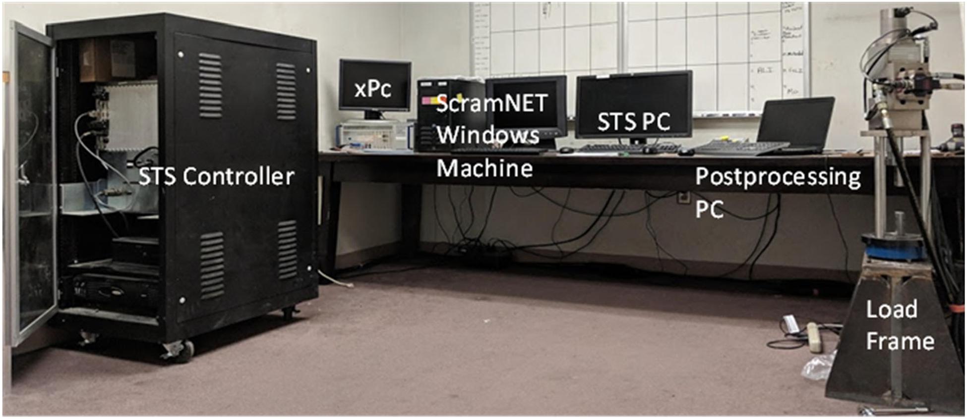
Figure 1. Compact HS/RTHS test setup at UNR.

The small-scale load frame is used for the experimental substructure in this setup with an actuator with 31.14 kN (7 kips) maximum load capacity and ±25.4 mm (±1 in) stroke. The actuator’s peak velocity at no load is 338.84 mm/s (13.34 in/s). The isolated hydraulic power supply system includes a pumping capacity of 8.71 lt/min (2.3 gpm), and the reservoir capacity of oil volume is 56.78 lt (15 gallons).

The FEM of the analytical substructures can be modeled in either OpenSees or Simulink. The setup is capable of running both real-time and slow (pseudodynamic) HS experiments. The slow HS case can be conducted using a predictor–corrector algorithm to control different time ranges that is defined in OpenFresco middleware (Schellenberg et al., 2009a, b). The host PC and xPC target machine have a TCP/IP connection to initialize and map the SCRAMNetGT memory locations. The xPC target machine is an environment that connects Simulink and Stateflow models to the physical components. The xPC solves Simulink-based analytical models. For the models other than Simulink, the analytical substructures are run from the host PC. For the applications where OpenSees/OpenFresco architecture is used, the xPC target is used as a middleware that transfers data between the analytical and experimental substructure. The calculated analytical substructure response is sent to the controller through the xPC target machine.

The STS controller has four channels that can control up to four actuators simultaneously, but using the current setup in Figure 1, only one channel is used to control one actuator. Displacement control is preferred for the actuator where computed displacement input controls the actuator, and the force feedback is measured and fed back to the physical substructure. It is important to mention that all HS components have SCRAMNetGT card, which uses shared memory locations with fiber optic communications to transfer data in real time. More details about the HS system development and verification where FEM is used can be found in Bas et al. (2020b).

In this research, this setup is used first with a simplified ML model, which is straightforward enough to model directly in Simulink. Therefore, no additional communication other than what is explained above is necessary. When a more complex ML model is introduced, some modifications and/or developments were sought on the communication side as explained later in Communication Development and Verification.

Modeling Assumptions and Training Dataset

A one-story, one-bay steel concentrically braced frame (CBF) with diagonal brace configuration was selected for the verifications and evaluations in this study. CBFs are convenient for the substructuring where the columns and beams of CBFs can be modeled with high accuracy, i.e., form the analytical substructure. Meanwhile, braces are better tested physically to accurately capture complex behavior such as buckling, and in turn, braces make the experimental substructure. A single small-scale brace can be tested as the experimental substructure in the used HS setup and can be combined with a prototype steel frame at full scale for the analytical substructure. For the sake of this study, a linear analytical model is first used, and then a heavily non-linear analytical substructure is considered for the advanced ML modeling. In both cases, no physical braces were used, and instead, a multiplier of the actuator’s actual achieved displacement is fed back to the RTHS loop to represent a hypothetical linear elastic test specimen as explained later. In other words, a non-linear experimental behavior was not considered in this study to make it simpler for verification purposes.

Figure 2 shows the CBF substructuring for HS testing. The analytical substructure involves two columns (W14 × 311), which are fixed at the base and a beam (W36 × 150) that has moment connections to the columns. The brace, on the other hand, has a pinned connection at both ends, where it works as an axial element. The bay width and the height of the frame are about 3.7 m. For this section, both columns and the beam are considered to be linear elastic. The mass and the damping are also considered to be a part of the analytical substructure. For simplicity in the validation and modeling purposes, the CBF is simplified as a single degree of freedom model. The mass of the system is selected to be 1.75 kN-s²/mm. The frame stiffness (analytical substructure stiffness) is calculated to be 176.75 kN/mm, where the axial brace stiffness is 1,224.1 kN/mm. The natural period of the system is calculated to be 0.294 s. A 2% Rayleigh damping is assumed to be the inherent damping of the structure. The pure analytical model of the overall system is developed in Simulink. The explicit integration algorithm provided by Chang (2009) is used to solve the equation of motion with 1/2,048-s time step. This explicit algorithm is unconditionally stable for linear systems and any instantaneous stiffness softening systems and conditionally stable for instantaneous stiffness hardening systems. Here, the time step of the controller and the integration algorithm are selected to be the same to synchronize the data transfer. The 1940 El-Centro ground motion acceleration (Figure 3A) was selected to be used for both training and HS testing purposes in this study.

FIGURE 2

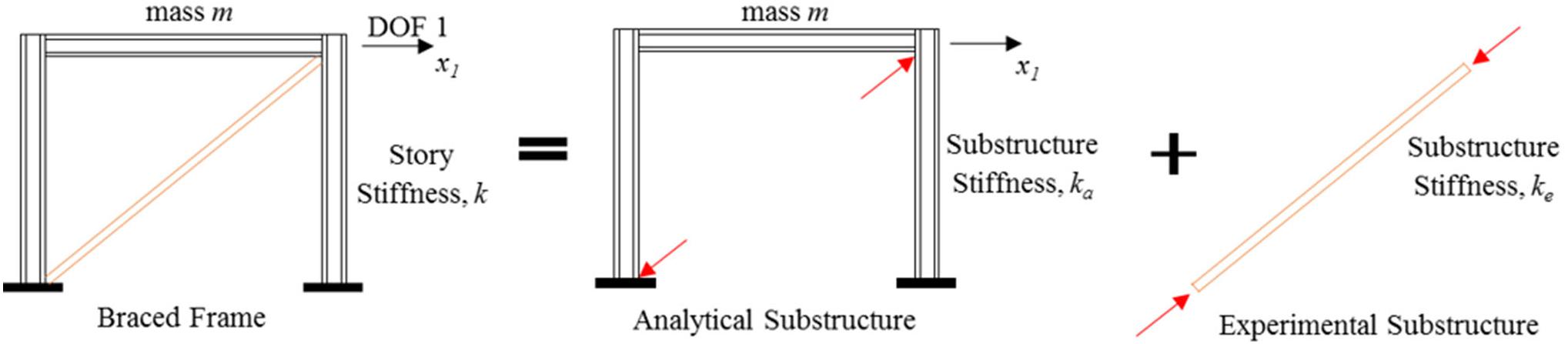
Figure 2. Model and substructuring of diagonal CBF for HS testing.

FIGURE 3

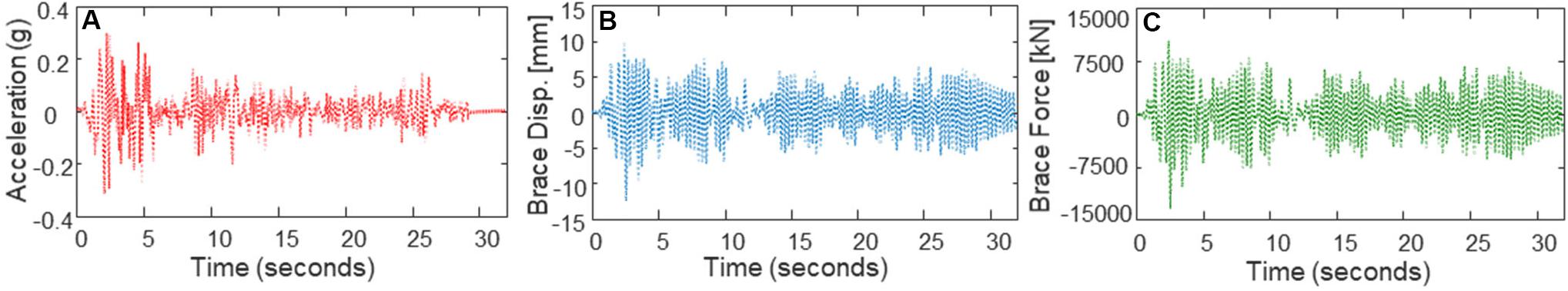
Figure 3. Datasets used for LR model training: (A) El-Centro ground motion acceleration, (B) brace displacement history, and (C) force history, both in local brace coordinates as obtained from the pure analysis.

As mentioned earlier, an LR method is used as a simplified metamodel for the first part of this study, which was trained by using a pure analytical solution of the CBF. An LR is one of the simplest ML algorithms that perform a task to make predictions based on the weighted sum of the input values and a bias term as a constant (Géron, 2017). The general equation is shown in Eq. 1, where $\widehat{\text{y}}$ is the predicted value, n is the number of the features, x_i is the i^th feature, and θ_j is the j^th model parameter (θ₀ is the bias term, where θ₁,θ₂,…,θ_n are the feature weights).

$\widehat{y}={\mathrm{\theta }}_0+{\mathrm{\theta }}_1{x}_1+{\mathrm{\theta }}_2{x}_2+\mathrm{\dots }+{\mathrm{\theta }}_n{x}_n(1)$

The training dataset was obtained from a pure analytical dynamic analysis of the overall system. The brace displacement and force time histories were obtained in local coordinates and used as training datasets in addition to the ground motion acceleration (see Figure 3 for these training components). Because the dataset is provided offline, the model is considered as batch learning. In total, five input features were selected to train the model to predict the output, which would be the command displacement of the experimental substructure of the HS system. The training features were selected to be (i) ground motion acceleration, (ii) displacement feedback value of the brace (from experimental substructure), (iii) force feedback value of the brace (from experimental substructure), (iv) one previous step of the predicted displacement, and (v) two previous steps of the predicted displacement. Because the pure analytical solution is used for the training dataset, an estimated 28-time-steps delay has also been considered to better represent the feedback that should come from the experimental substructure. However, to obtain a more accurate delay estimation better than the assumed 28-time steps, the trained model was run in the HS setup first without including the actuator’s feedback, which were obtained to be used in the next training phase. Then, a more refined model was generated by using these “real” displacement and force feedback data with the other three features.

A brief overview of how the LR training was conducted is as follows. In this study, the “Regression Learner” app in MATLAB, which is under the ML group, was used to train the LR algorithm. First, the predictors and response were defined, and then a validation method was selected. The cross-validation with five folds was selected to protect the model against overfitting by partitioning the datasets into folds and estimating the accuracy of each fold. A session was started next for training, and an LR model was selected. Afterward, the model training was done, and the model root mean square error (RMSE) values were checked. Once the model was trained, the model was exported to the workspace to obtain the LR parameters to make new predictions. After getting the parameters, a Simulink model was generated to represent the HS case where at every step the predicted displacement is calculated, and the determined force feedback is fed back to the system to make new predictions.

RTHS Test Results

Once the model is trained for the features explained above, a Simulink model with MATLAB function was prepared to represent the LR model but was first assessed against the pure analytical FEM solution. The developed LR model formulation is shown in Eq. 2, where x is represented as displacement of the brace, F is the force of the brace, and ẍ_g is the ground motion acceleration. Table 1 shows the model parameters that belong to the trained model.

TABLE 1

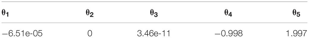
Table 1. LR model parameters.

$$\begin{array}{c}{x}_{prediction,i+1}=f({\stackrel{\mathrm{..}}{x}}_g,x_{feedback,i},F_{feedback,i},x_{prediction,i},\\ x_{prediction,i-1})\\ ={\text{θ}}_1{\stackrel{\mathrm{..}}{x}}_g+{\text{θ}}_2{x}_{feedback,i}+{\text{θ}}_3{F}_{feedback,i}\\ +{\text{θ}}_4{x}_{prediction,i}+{\text{θ}}_5{x}_{prediction,i-1}\end{array}(2)$$

The brace displacement response of the FE model and the prediction from the LR metamodel were compared as the two alternative pure analytical solutions. The FE model response was considered to be the exact solution, and in turn, a normalized RMSE (NRMSE) was calculated to evaluate the comparison. It should be noted that for the pure analytical response, because there is no feedback from the actuator included yet, the displacement feedbacks are generated using 28-time-steps delay as discussed earlier. Figure 4 shows the comparison between the pure analytical brace displacement response of the FE model and the LR model. The NRMSE value was calculated as 0.15%, which confirms that the LR prediction can be used further.

FIGURE 4

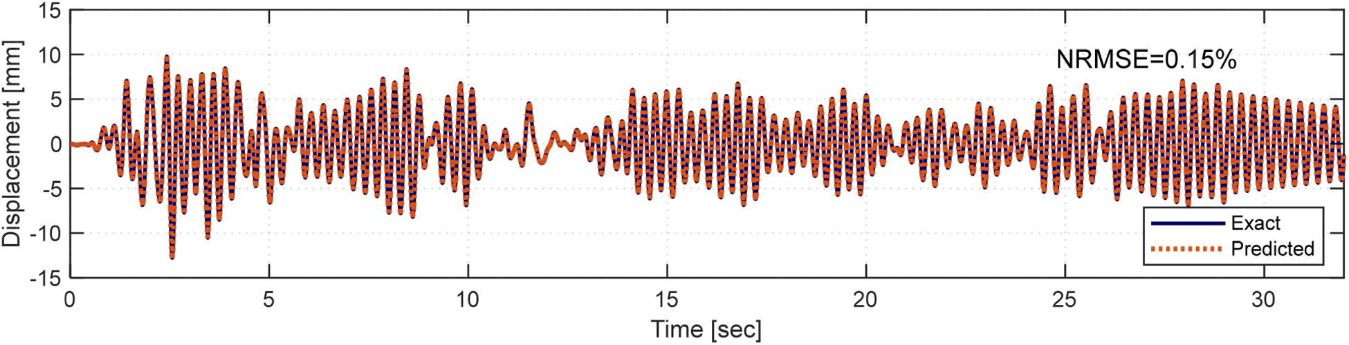
Figure 4. Comparison of the brace displacement time histories from FE model and LR metamodel.

Moreover, for complete evaluation of using the LR model, RTHS validation tests were conducted using the LR model and compared to the pure analytical FE solution. The validation tests were considered for a hypothetical linear elastic experimental specimen where the displacement command was multiplied with the constant stiffness value of the specimen to represent a force feedback value. The verified MATLAB-based LR metamodel explained above was then compiled in the xPC Target machine. Two types of RTHS tests were conducted, namely, offline and online RTHS tests. The offline test is where the feedback from the experimental model is taken from the command of the system’s controller, i.e., without actually moving the actuator. For the offline RTHS test, again, instead of using the actual actuator’s feedback, the command displacement value was used with a 28-time step delay from the predicted displacement value. Figure 5A shows the brace displacement time history comparison for the pure analytical model and from offline RTHS with the LR metamodel. The NRMSE value was calculated as 0.15%, which is very reasonable given the simplicity of the problem and test.

FIGURE 5

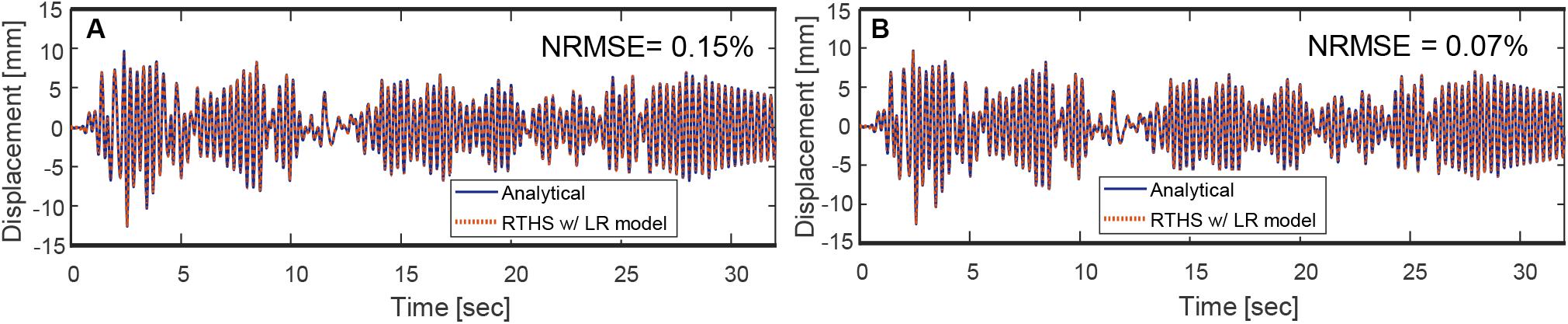
Figure 5. Results from (A) offline and (B) online RTHS with the LR metamodel and validation against pure analytical solution.

Next, an online test was considered where the hydraulic system is turned on and the actuator was moved, and the actual feedback was fed into the analytical model. This is to test the capability of the metamodel to derive the actuator in the closed loop RTHS setting. The displacement value was obtained from the actual actuator displacement, and again the force feedback was obtained from a constant stiffness to mimic a linear elastic specimen. For such tests, the ATS compensator mentioned above (Chae et al., 2013) was used to compensate for the actuator delay. Figure 5B shows the online RTHS results for brace displacement comparison with the pure analytical model. The NRMSE value was calculated to be 0.07%, which verifies the acceptable performance of the metamodel-driven system. It is noted that the conducted test considered linear elastic analytical and hypothetical experimental substructures. Thus, the dynamic response was accurately obtained from pure analytical solutions and in turn accurately trained the LR metamodel. So, the low error is not meant to assess the quality of LR metamodel predictions, but rather confirm the performance of the overall RTHS hardware and communication system.

Such simple linear elastic case was possible to easily model with the LR algorithm, which was also simple enough to code using MATLAB and Simulink functions and directly compile it into the RTHS hardware. However, the modeling capacity of LR models is rather limited and cannot be used for complex non-linear systems. Thus, more complicated ML algorithms are likely to be used to push the boundaries of future RTHS testing, which motivated the next part of the study. More complex ML algorithms such as deep learning were considered, which required integrating Python into the RTHS loop. Developing the ML models for the next phase of validation is the focus of the next section, which is then followed by the communication schemes development and verification for RTHS with Python-based complex ML models.

Advanced ML Techniques for RTHS

This section provides first a brief overview of more complex ML models, which includes the LSTM model used in this study. The section also provides more details on LSTM model features, training sets used for this study, and sensitivity analysis to understand the performance of the model as it pertains to the structural modeling problem in hand.

One of the subgroups of ML methods is deep learning, which uses neural networks with many layers. Deep learning studies deep neural networks, which is a form of stacking several layers of ANNs. The most straightforward architecture of ANN is the perceptron, which takes the weighted sum of the inputs and then multiplies this sum with an activation function and outputs the result. The perceptrons are not capable of learning complex patterns; thus, multilayer perceptron (MLP), which is a stacked version of multiple perceptrons, is suggested to improve some of the limitations. This type of ANNs contains one input layer, one or more hidden layers, and an output layer. For these models, the input-to-output flow is only one way, which represents a feedforward neural network. An ANN has simple architecture and is used for both classification and regression problems. However, more advanced models developed recently, such as CNN and RNN, offer more opportunities while modeling non-linear structural responses due to their impressive feature extraction (Zhang et al., 2019b).

Convolutional neural networks are a family of deep learning, which is mostly used for image classification. However, they are also capable of handling long sequence data for regression analysis (LeCun and Yoshua, 1995). The architecture of CNN is inspired by the brain’s visual cortex, which uses the function of pattern connectivity function that the brain has. CNN has two different layers than the regular ANN, which are convolutional layers and pooling layers. The most critical difference in CNN is the convolutional layer, where the previous layer’s inputs are only connected to their receptive fields, which defines the neurons’ weight. By using this feature, the network hierarchically splits the input features, and each neuron analyzes the small region of the image. On the other hand, the pooling layer aims to subsample the image, which also reduces the computational load and the possible overfitting. These advances separate CNN from other deep neural networks because it is beneficial on large inputs by reducing the connections and correspondingly the training parameters.

The other crucial neural network is RNN, which has connections to the previous input points. The difference of the RNN from previously defined neural networks is these backward connections where the previous ones are feedforward neural networks. The architecture of the RNNs includes a recurrent neuron which receives the output from the previous time step with the input. This allows this type of network to be capable of time-series forecasting. Although it is successful in sequence datasets, the method has two main disadvantages for longer sequences: (i) unstable gradients and (ii) utilizing a very limited short-time memory (Bengio et al., 1994). To overcome these problems, the LSTM cell was proposed, which can detect long-term dependencies, rapidly converge, and perform better (Hochreiter and Jürgen, 1997).

In this study, the LSTM networks were selected and used for the purpose of modeling and dynamic response prediction of the analytical substructures needed for the sought communication schemes development and RTHS demonstration. The modeling assumptions, training, and model tuning are explained in detail in the following sections.

LSTM Networks

The LSTM networks were developed, especially to answer the need in long sequence datasets. Figure 6A shows a typical deep LSTM network, with input, hidden, and output layers. The architecture of an LSTM cell is shown in Figure 6B. In particular, an LSTM cell includes h_(t) and c_(t) apart from inputs (x_(t)) and outputs (y_(t)), which are representing short- and long-term states, respectively.

FIGURE 6

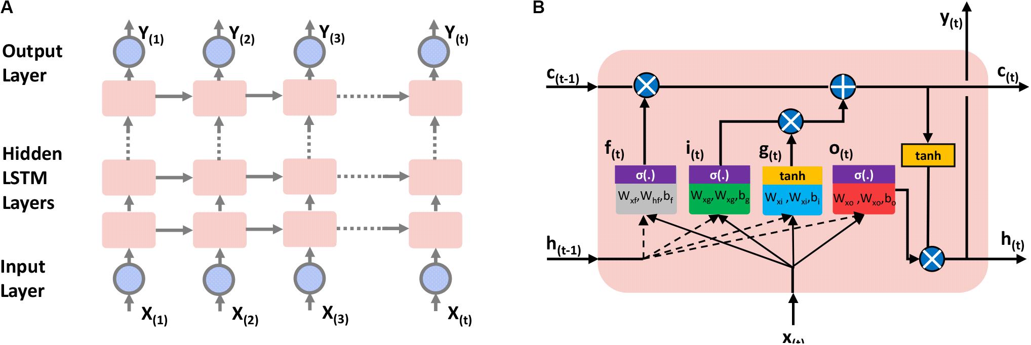
Figure 6. (A) A deep LSTM network through time, (B) LSTM cell architecture.

In each time step, the LSTM cell receives two input vectors that are the current time step input vector x_(t) and previous time step output vector h_(t–1) (which is also y_(t–1)) and fed into four different fully connected layers. The output of g_(t) analyzes these two inputs, which is the weighted sum of the inputs followed with an activation function (tanh function). A regular RNN cell only has this feature, which directly gives the output. However, in the LSTM cell, three other layers, which are the gate controllers, help control the memory information. These three gates use logistic function, σ(.), as an activation function where the output changes from 0 to 1. The forget gate (output of f_(t)), is where the unnecessary parts of the long-term state are erased. On the other hand, the input gate (output of i_(t)), controls the parts of g_(t) to be added in the long-term state. Lastly, the output gate manages the parts of the long-term state that should be read and output to both h_(t) and y_(t). The LSTM computations are briefly outlined and given in Eqs 3 through 8. In these equations, the input vector of the current state x_(t) in each layer is connected with the weight matrices of each layer W_xi, W_xf, W_xf, and W_xf, where the previous short-term state vector h_(t–1) is connected to their layers with the weight matrices of W_hi, W_hf, W_hf, and W_hf. In each layer, b_i, b_f, b_o, and b_g are the bias terms. Lastly, ⊗ is the element-wise multiplication. It should also be noted that, as suggested by Jozefowicz et al. (2015), the bias term of the forget gate (b_f) is initialized as “1”s to prevent forgetting everything at the beginning of the training.

${\mathbf{\text{i}}}_{\left(t\right)}=\mathrm{\sigma }\left({\mathbf{\text{W}}}_{xi}^T{\mathbf{\text{x}}}_{(t)}+{\mathbf{\text{W}}}_{hi}^T{\mathbf{\text{h}}}_{(t-1)}+{\mathbf{\text{b}}}_i\right)(3)$

${\mathbf{\text{f}}}_{\left(t\right)}=\mathrm{\sigma }\left({\mathbf{\text{W}}}_{xf}^T{\mathbf{\text{x}}}_{(t)}+{\mathbf{\text{W}}}_{hf}^T{\mathbf{\text{h}}}_{(t-1)}+{\mathbf{\text{b}}}_f\right)(4)$

${\mathbf{\text{o}}}_{\left(t\right)}=\mathrm{\sigma }\left({\mathbf{\text{W}}}_{xo}^T{\mathbf{\text{x}}}_{(t)}+{\mathbf{\text{W}}}_{ho}^T{\mathbf{\text{h}}}_{(t-1)}+{\mathbf{\text{b}}}_o\right)(5)$

${\mathbf{\text{g}}}_{\left(t\right)}=tanh\left({\mathbf{\text{W}}}_{xg}^T{\mathbf{\text{x}}}_{(t)}+{\mathbf{\text{W}}}_{hg}^T{\mathbf{\text{h}}}_{(t-1)}+{\mathbf{\text{b}}}_g\right)(6)$

${\mathbf{\text{c}}}_{\left(t\right)}={\mathbf{\text{f}}}_{\left(t\right)}\otimes {\mathbf{\text{c}}}_{\left(t-1\right)}+{\mathbf{\text{i}}}_{\left(t\right)}\otimes {\mathbf{\text{g}}}_{\left(t\right)}(7)$

${\mathbf{\text{y}}}_{\left(t\right)}={\mathbf{\text{h}}}_{\left(t\right)}={\mathbf{\text{o}}}_{\left(t\right)}\otimes tanh\left({\mathbf{\text{c}}}_{\left(t\right)}\right)(8)$

Briefly, an LSTM cell can observe the input importance, remember the long history of time series while storing them in the long-term state, and store longer information as long as it is needed and remove whenever it is unnecessary. Therefore, even if the problem is highly non-linear, the LSTM is capable of capturing long-term patterns in the time series (Zhang et al., 2019b).

Training Datasets

A similar one-story, one-bay steel braced frame as discussed in Simplified Machine Learning Model for RTHS, but with some modifications, was selected for this part of the study for generating training datasets. The analytical substructure was designed to be non-linear for the RTHS tests where this non-linear analytical substructure is to be represented with an advanced ML model. Again, the main goal of this fundamental study is to explore validity of using ML modeling for RTHS and develop/verify the needed communication schemes. Hence, the experimental element was selected to be linear elastic so that it can be still combined with the non-linear analytical substructure to obtain pure analytical solutions for validating the RTHS tests.

The pure analytical model of the overall system was modeled in OpenSees (McKenna et al., 2000), which offers a wide range of material models, elements, and solution algorithms. The columns (W36 × 150) and beam (W14 × 311) elements were defined using fiber sections with non-linear material behavior as illustrated in Figure 7. The non-linear material behavior was defined with Steel02 material in OpenSees (Figure 7C), which is uniaxial Giuffre–Menegotto–Pinto steel material with isotropic strain hardening (Filippou et al., 1983). The implicit Newmark method was used for all the conducted analysis to obtain the training dataset, and the parameters were set as γ = 0.50 and β = 0.25.

FIGURE 7

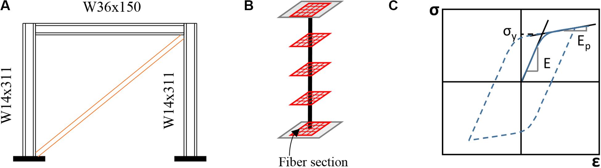
Figure 7. (A) Pure analytical model of the CBF, (B) distributed plasticity with fiber sections for non-linear elements, (C) steel 02 model stress–strain relationship.

The yield stress of the material was selected to be 345 MPa with modulus of elasticity of 200 GPa. On the other hand, the brace, which is the experimental substructure in the RTHS tests, was modeled to be linear elastic with axial stiffness of 278 kN/mm. The choice of the brace stiffness allowed the CBF to experience larger displacements and higher non-linearities to provide a wider range of behavior for training the ML model. The mass of the system was selected to be 1.75 kN-s²/mm. The natural period of this CBF system was calculated to be 0.47 s. A 2% Rayleigh damping was assumed for modeling the inherent damping of the structure.

The non-linear time history analysis of the pure analytical model of the overall system was obtained using the implicit Newmark method (average acceleration), which is considered the “correct” solution for the further investigation and validation in this study. A proper convergence study was carried out, and the time step for the integration was selected to be 0.02 s, which is also equal to the ground motion time step. The 1940 El-Centro earthquake was selected again for this part. While the duration of the earthquake record is 31.2 s, the analyses were carried out for full 32 s, which generated 1,600 data points for each response.

The training dataset for the deep LSTM model of the non-linear analytical substructure was selected to be the ground motion acceleration and brace force time histories. The brace axial displacement in local coordinates, i.e., the scaled actuator command in the used substructured test setup shown in Figure 2, was selected to be the output for the model training purposes. This is to be later sought as the ML model output or prediction when in the RTHS loop. Thus, the ML model used two inputs to give the brace displacement command prediction to the experimental substructure. It should be noted that, during an online RTHS test, the system is a closed-loop one, and the brace force is dependent on the predicted brace displacement. This dependence between the input and output brings a high level of uncertainty, and the model can become unstable even in the pure analytical examination of the model.

Moreover, the experimental setup can also bring addition sources of errors and uncertainties due to the nature of the servo hydraulic system. Therefore, a systematic error, which is referred to as bias here for simplicity, was introduced to expand the training environment. This bias is added only to the brace force time history and is meant to account for unforeseen experimental errors and metamodel non-linearity due to input output correlation. For instance, the ML model is trained to predict, for example, a 25-mm displacement output value for 25-kN force feedback input and 0.25-g ground motion excitation. However, the actual force feedback looped back to the ML model during the RTHS test and needed to make the next prediction for the 0.25-g ground motion acceleration could be 26 kN instead of 25 kN because of the experimental errors. Thus, for the ML model to still predict the intended 25-mm displacement, it needs to have been trained that at 0.25-g ground motion input, the force could be 25 or 26 kN or something else. For this purpose, additional force histories where generated using ± 5, ± 10, ± 15% of the brace force and were added to create the biased dataset.

The original dataset along with the six conceived datasets with the added bias were stacked together for the overall training dataset. This required the same ground motion to be repeated seven times to go with the seven cases of force input to prepare the ML model that, for a given ground motion input, the force could have one of seven possible values based on the devised bias. This training scheme resulted in a total of 11,200 data points for the force input and the seven-times repeated ground motion input. The stacked ground motion acceleration, i.e., Input 1, and the stacked force time history of the brace, i.e., Input 2, are shown in Figures 8, 9, respectively. The stacked brace displacement dataset obtained from the OpenSees analysis and used to represent the output of the training is shown in Figure 10.

FIGURE 8

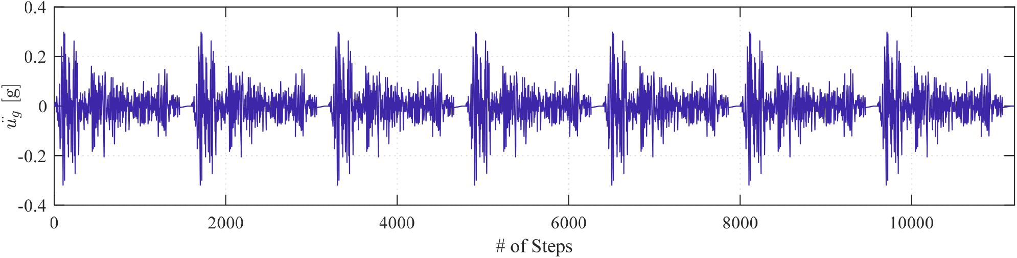
Figure 8. Stacked ground motion acceleration dataset (Input 1).

FIGURE 9

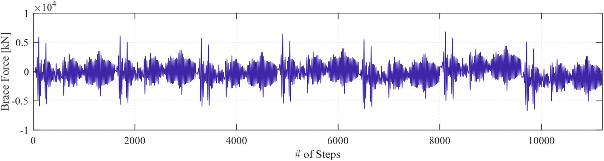
Figure 9. Stacked brace force dataset (Input 2).

FIGURE 10

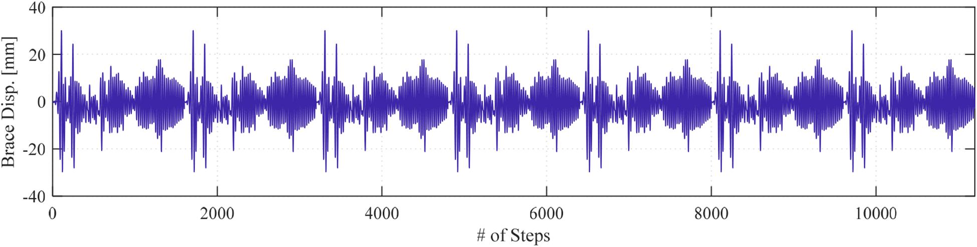
Figure 10. Stacked brace displacement dataset (output).

Once the training dataset is generated, it should be modified and reshaped to be able to train the LSTM model. The input sequences of LSTM networks are formatted to be three-dimensional (3D) arrays, as in other time-series prediction models (Géron, 2017) and as illustrated in Figure 11. The first dimension is the batch size or the number of samples of the dataset. The second dimension is the lookback, which defines how many past time steps that the model should get. Finally, the third dimension is the size of the input dimension or number of features. The lookback parameter is one of the key parameters that should be tuned carefully as it makes LSTMs more reliable because it allows the algorithm to look back in the past time steps to make better future predictions. Although it extends the used information, it might increase the memory requirements. On the other hand, the output shape can be either 2D or 3D arrays, which depends on the return sequences. Generally, in between the layers of the deep LSTM network, the return sequence is set to be true except for the last layer, which means the final output contains a single output value per time step. For this study, the 2D data format was considered for the output shape of the model.

FIGURE 11

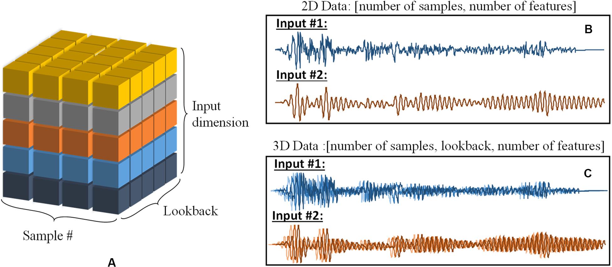
Figure 11. (A) Schematic representation of 3D data format, (B) input dataset in 2D format, and (C) input dataset when reshaped into 3D format.

Figure 11A shows a schematic representation of the 3D data format, where each color represents different input feature (input dimension). In this study, the number of features is two, i.e., Input 1 and Input 2, as mentioned earlier. In Figure 11B, these two inputs are represented in 2D data shape, and Figure 11C presents the reshaped version of the data. For simplicity, only one ground motion and corresponding brace force time history are shown in the figure instead of a full stack of the input datasets.

Implementation Methodology and Sensitivity Analysis for LSTM Model

The deep LSTM model used in this study was trained and generated in the Python environment using Tensorflow 2.0 framework, which is a high-performance computing library introduced by Google (Abadi et al., 2015). Tensorflow offers many packages and features, and one of the most popular ones it supports is Keras (Chollet, 2015). Keras is a high-level Application Program Interface that is highly attractive for building and training deep learning models. Generating workflows in Keras is simple because there are several standalone modules, such as neural layers, optimizers, cost functions, and user-defined modules. Thus, one can easily connect and stack these modules to generate an ML model. The inputs and output training datasets were fed into the deep LSTM models to tune the hyperparameters, i.e., size of the hidden layer, number of layers, number of neurons, batch size, lookback size, number of epochs, learning rate, etc. To train a large deep neural network, a faster optimizer should be used because the training time can take longer. The Adam (Adaptive Moment Estimator) optimizer was selected to train for the models used in this study, with a learning rate of 0.001, because it is computationally efficient and well-suited for problems with large datasets (Kingma and Ba, 2015). The number of epochs was set to be 10³. Moreover, the model was trained to minimize the cost function defined in Eq. 9, which is mean square error (MSE) between the given displacement values (x_n) and the predicted displacement values (${\widehat{x}}_n$).

$J\left(\mathrm{\theta }\right)=MSE=\frac{1}{N}\sum _{n=1}^N{\left(x_n-{\widehat{x}}_n\right)}^2(9)$

In this study, several layer numbers with different sizes of hidden layers were evaluated. The models had an input layer, four LSTM layers with 30 units in each layer, and one dense layer, which is a fully connected layer that outputs the prediction. For these models, different lookback values, i.e., 1, 5, 10, 15, and 20, were selected to select and fine-tune the most accurate model to be used as computational substructure in the RTHS loop. Moreover, 70% of the dataset was set to be the “training” part of the dataset, and the rest was used as the “test” dataset. The brace displacement response prediction values from the LSTM models with different lookback values were compared against the pure analytical model response. The performance of the model prediction was evaluated using the NRMSE, normalized energy error (NEE), and maximum amplitude error (MAE) given in Eqs 10 to 12. The NRMSE is an adequate way of evaluating the overall model performance, whereas the NEE and MAE are more focused on amplitude errors between the datasets.

$\text{NRMSE}=\frac{\sqrt{\frac{1}{N}{\sum }_{n=1}^N{\left(x_n-{\widehat{x}}_n\right)}^2}}{\max \left(\widehat{x}\right)-\text{min}\left(\widehat{x}\right)}(10)$

$\text{NEE}=\left|\frac{{\sum }_{n=1}^N{\left(x_n\right)}^2-{\sum }_{n=1}^N{\left({\widehat{x}}_n\right)}^2}{{\sum }_{n=1}^N{\left({\widehat{x}}_n\right)}^2}\right|(11)$

$\text{MAE}=\left|\frac{\text{max}(\left|x\right|)-\text{max}(\left|\widehat{x}\right|)}{\text{max}(\left|\widehat{x}\right|)}\right|(12)$

For the pure analytical assessment of the metamodel response, there was no real feedback from the actuator. That is because the brace force used as input for the model at a given time step was obtained from multiplying the predicted displacement response from previous step by the axial stiffness of the brace. Table 2 summarizes the performance evaluation of the deep LSTM models with different lookback values. It can be seen from the error calculations and the plots that the model trained with only one lookback data has the worst performance compared with the others. When this value was increased to five, the model performed slightly better in terms of amplitude; however, the prediction resulted in a very noisy signal. The models trained and evaluated with 10, 15, and 20 performed relatively close to each other. However, the model with 15 lookbacks stood out for best performance. The LSTM models with 15 and 20 lookbacks, referred to as Model 1 and Model 2, respectively, were selected and used for the validation and demonstration RTHS tests.

TABLE 2

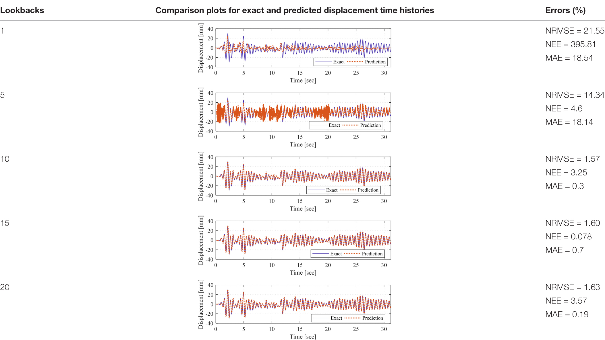
Table 2. Deep LSTM model comparison for different lookback values.

Communication Development and Verification

One of the critical aspects of HS/RTHS is the proper data communication between the analytical substructure and experimental substructure. The UNR setup components and configuration information are given above in HS System Components. As mentioned earlier, the analytical substructure of the HS/RTHS tests can be modeled in either Simulink directly or in an FE software such as OpenSees along with a middleware such as OpenFresco (Schellenberg et al., 2009a). OpenFresco is a software that connects FE models to the controllers and data acquisition systems in laboratories to enable HS. It allows interfacing different computational drivers. In this study, a novel communication scheme was developed to connect the Python-based models to the HS/RTHS loop via OpenFresco as a middleware. The authors have previous experience in developing and verifying new HS communication schemes that also used OpenFresco (Moustafa and Mosalam, 2015a, b).

To assess the online performance of the LSTM models in providing a prediction and in anticipation of future models that could be more complex and larger in size, two scenarios for calling the LSTM models were considered and tested. The first case used a local PC that was physically part of the RTHS, and the second considered a high-performance computing cluster. The communication details for Python-based metamodel substructures when located in local PC (host PC) are presented first.

Figure 12 shows the hardware components and the communication details schematically. In this configuration, Python is located at the host PC, where the xPC connection and the SCRAMNetGT initializations are made. Python can be run either from the command prompt (i.e., python.exe) or Anaconda prompt or Jupyter notebook. The OpenFresco architecture for Python connection is the “client&middle-tier server,” where OpenFresco serves as a middle-tier server, and Python is the client. At the OpenFresco side, the server is started by opening a UDP/TCP channel, and the simulation application site is set. On the other hand, Python has a “socket” module to set the connection and send and receive data with either TCP or UDP protocols. In this study, the data communication between Python and OpenFresco is provided with the UDP communication protocol. The experimental site is also connected with this middle-tier server, which is a local experimental site in this study. Moreover, the experimental control, which is the interface with the laboratory hardware system, should be defined. This is where the data to/from the controller through the xPC target are transferred. The connection between the host PC and the xPC Target can be set up with either TCP/IP or SCRAMNetGT connection. The SCRAMNetGT connection was considered here because it provides more stable and faster data transfer.

FIGURE 12

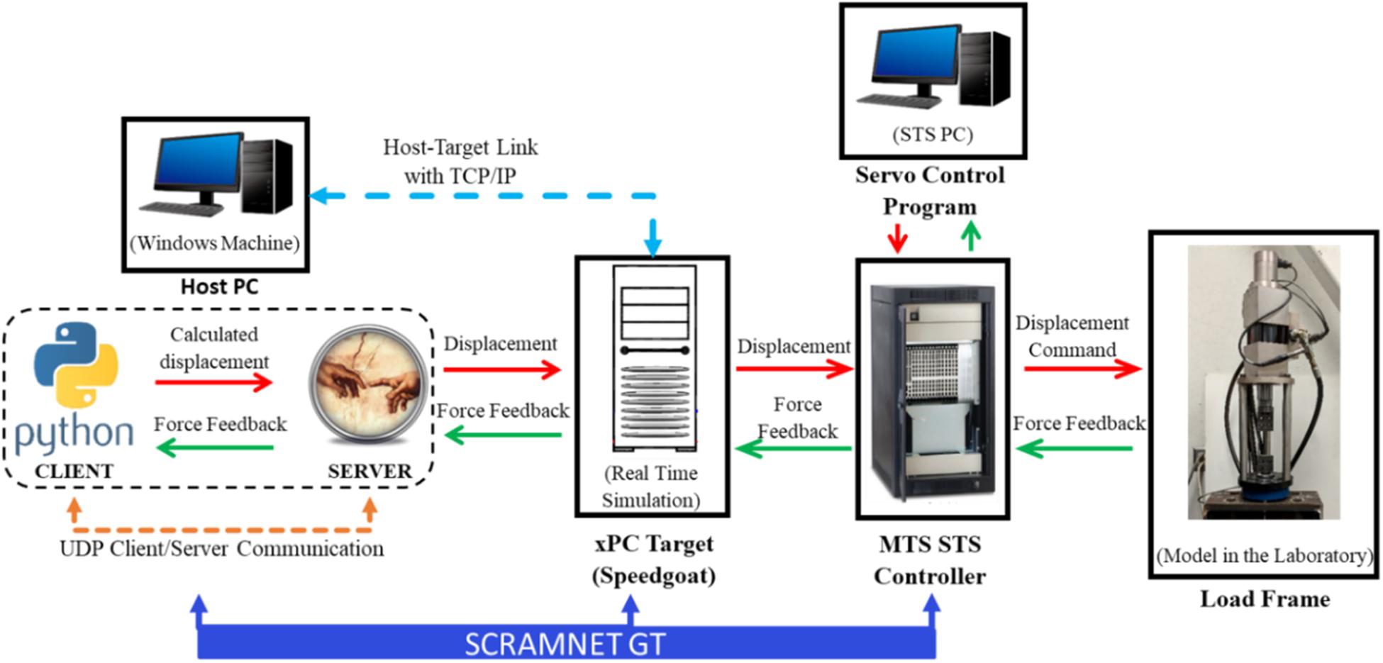
Figure 12. HS/RTHS communication details for Python-based analytical substructure (metamodel) located and called from local PC.

The communication details when a high-performance computer cluster is considered are provided next. The cluster that has been used in this study belongs to UNR’s Department of Computer Science and Engineering and used for teaching and simple research studies. Python packages and modules can be run from a cluster, especially when complicated calculations are needed to be done at high speeds. For this communication, Python models were run in the cluster, while OpenFresco is in the host PC. The cluster and the host PC were connected through the Secure Shell (SSH) network protocol. The data transfer was performed with UDP tunneling through the SSH connection. The schematic communication details of this configuration are shown in Figure 13. Other than this, the data transfer procedure is the same as it is explained for local PC.

FIGURE 13

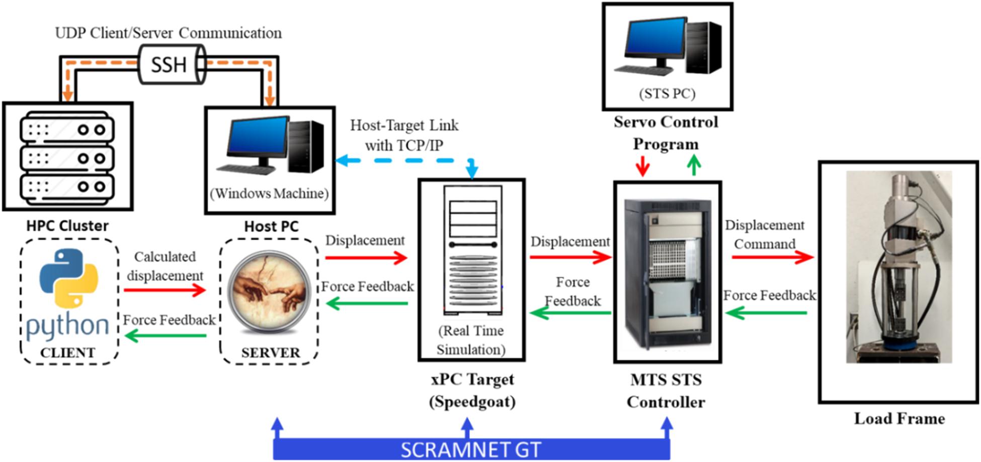
Figure 13. HS/RTHS communication details for Python-based analytical substructure (metamodel) located at and called from high-performance computer.

The overall concept of the data transfer in this RTHS setting is as follows. The trained deep LSTM network model (metamodel), which is the analytical substructure of the RTHS test, runs from Python. Python can be run from either the local PC or the cluster. At each time step, this metamodel calculates the input displacement and sends it as displacement command to the experimental substructure. Then, the experimental substructure sends the measured force from the specimen and feeds it back to the metamodel. OpenFresco has a predictor–corrector algorithm, which is programmed in Simulink and Stateflow, and runs in the xPC target machine to manage the real-time environment, which synchronizes the integration time step, the simulation time step, and the controller time step (Schellenberg et al., 2009b). The predictor–corrector algorithm generates smooth command signals at the same rate as the control system base clock frequency, and this allows generating displacement targets from the non-deterministic rate numerical models (Serebanha et al., 2019). For real-time tests, the simulation time step should be equal to the integration time step. During the RTHS, the numerical model solves the new target displacement, and the predictor–corrector algorithm generates command displacements based on polynomial forward prediction. The new target displacement should be calculated and sent within 60% of the simulation time step to allow the remaining time frame for data transfer for RTHS. If this is not satisfied at a single point, then the predictor–corrector provides a solution with slowing down the command displacement until the new target is received (Serebanha et al., 2019). In the proposed system with metamodels, i.e., no integration for the equation of motion is needed, the integration time becomes the prediction time step. The prediction time step was set to be 0.02 s, which was the same as the training time step.

The validation for the aforementioned communication scheme is first tested between the computer and controller and checked against the pure analytical case. For this validation scenario, offline RTHS tests were conducted while the hydraulic system was off. Because no actual actuator feedback was available yet, the force feedback was obtained from the command of the system, where the stiffness multiplier was applied to the displacement command, as opposed to the actual actuator feedback in online tests. It is noted again that for all tests considered in this study, a linear elastic experimental substructure was considered through the stiffness multiplier to make it possible to compare with pure analytical cases for verification. The offline RTHS test results are presented in Figures 14A,B for the deep LSTM network model with 15 and 20 lookbacks, i.e., Model 1 and Model 2, respectively, located at the local PC. Moreover, Figure 15 shows the same comparisons for the RTHS tests that were conducted from the cluster. The RTHS test results, i.e., brace displacement, were compared with the pure analytical response to estimate NRMSE, NEE, and MAE. All error values from for both experiments are provided in the figures. The figures show that Model 2 with 20 lookbacks had overall less NRMSE and MAE values than Model 1. However, for all cases, the RTHS results were very comparable to the pure analytical solutions, which verifies the real-time communications for both host PC and the cluster.

FIGURE 14

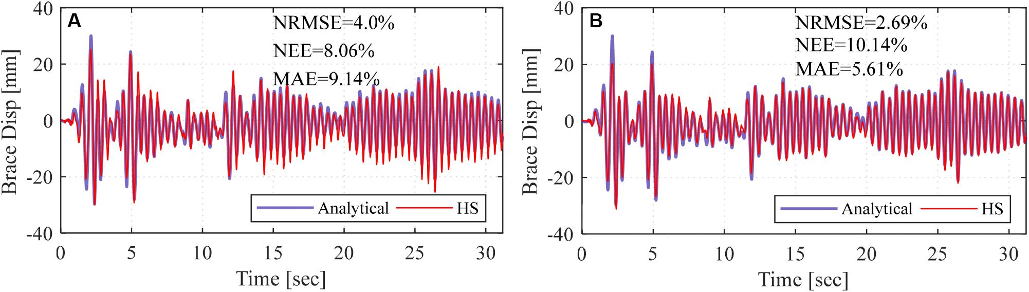
Figure 14. Brace response from pure analysis and offline RTHS tests with deep LSTM network model located at local PC and trained using (A) 15 and (B) 20 lookbacks.

FIGURE 15

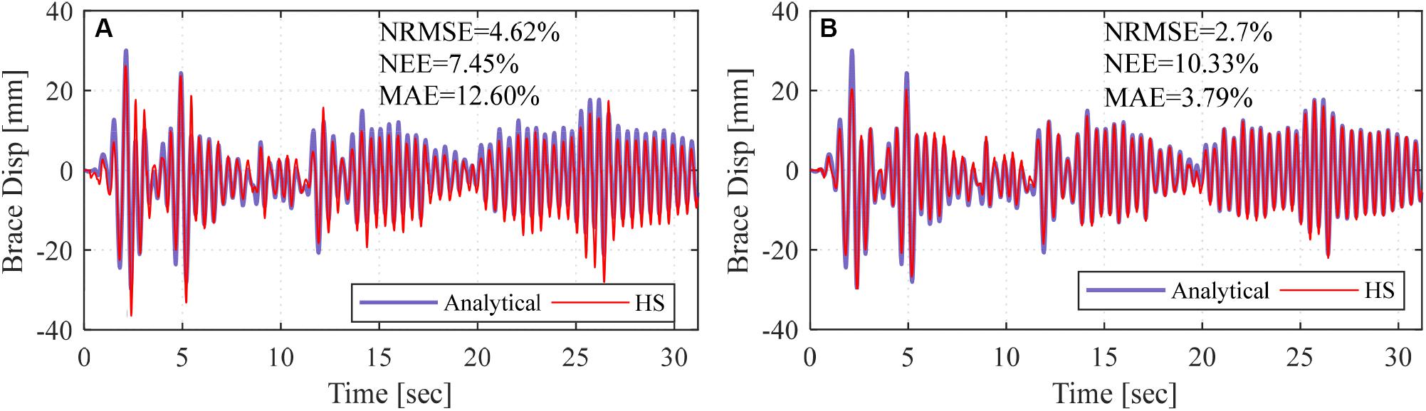
Figure 15. Brace response from pure analysis and offline RTHS tests with deep LSTM network model located at high-performance computer cluster and trained using (A) 15 and (B) 20 lookbacks.

Online RTHS Tests

In this section, the deep LSTM network models with lookbacks 15 and 20 are further used to evaluate the ML-based RTHS approach and communication among different components using full online tests. Thus, for all the RTHS tests that are presented and discussed in this section, the hydraulic system was on with the actuator free to move, and in turn, actual feedback from the actuator was obtained and fed into the analytical substructure. At each time step, the actual achieved actuator’s displacement was modified using the constant brace stiffness multiplier to feedback an equivalent, yet representative, force feedback of a linear elastic experimental substructure. Different geometric scales (S_L) were considered for the mock experimental specimen to test the RTHS system and ML-driven actuator at wide range of displacements and velocities for better assessment. The relevant considered scale factors were S_L for length and S_L² for the force values, and these scale factors are controlled through Simulink blocks that are compiled in xPC Target. Several tests were conducted, and the respective discussion is presented in three subsections to make proper comparisons. First, results from online RTHS with conventional non-linear FE models are presented to serve as reference for ML-based tests verification. Next, computational time is evaluated and compared for RTHS test results with the ML model located at local PC and cluster to explore whether there are benefits in using cluster as opposed to local PC. Finally, the RTHS tests that used local PC are discussed further through comparisons against both RTHS tests with FE models and the pure analytical solution. A total of 40 different online RTHS were conducted with different geometric scales, varying LSTM models, and with or without using a dedicated time delay compensator. Selected results are shown, but all error calculations (NRMSE, NEE, and MAE) for the 40 tests are summarized and discussed in the last subsection.

Online RTHS With FE Model

Conducting RTHS with large or heavily non-linear analytical substructure models could be challenging and has limitations that could be mostly associated with insufficient computational time within the RTHS loop. For example, when both stiffness and strength degradation are considered, direct integration methods were found to have some limitations, only for RTHS (Bas and Moustafa, 2020). The idea of using an ML approach or metamodels could eliminate such limitations, which is the motivation behind this study. Thus, the system capabilities and online RTHS tests are first evaluated with the FE model. For these tests, OpenSees was used to model the analytical substructure. The model properties and modeling assumptions were the same as given in Training Datasets. For the experimental substructure, several length scale factors were considered at 5, 10, 15, 20, and 25. All tests were conducted in real time where both the integration and simulation time steps were set to 0.02 s. The integration algorithm was selected to be the explicit KR-α (Kolay et al., 2015). Two sets of tests were conducted with and without using the ATS compensator to correct for the actuator delay. The KR-α integration and ATS compensator initial parameters that were used in the RTHS tests are listed in Table 3. A side convergence study was conducted to obtain the best input value for one of the integration parameters, i.e., ρ_∞, as illustrated in Figure 16. The brace displacement time histories were obtained for different ρ_∞ values, and the NRMS errors were calculated for assessment. Although there were no significant differences between 0.75 and 1.0, the ρ_∞ was assigned to be 1.0 because this was the case that corresponded to the least error. All tests were compared against the pure analytical solution of non-linear CBF, which used implicit integration methods and considered to be the “correct” solution when only the brace is considered linear elastic as explained before.

TABLE 3

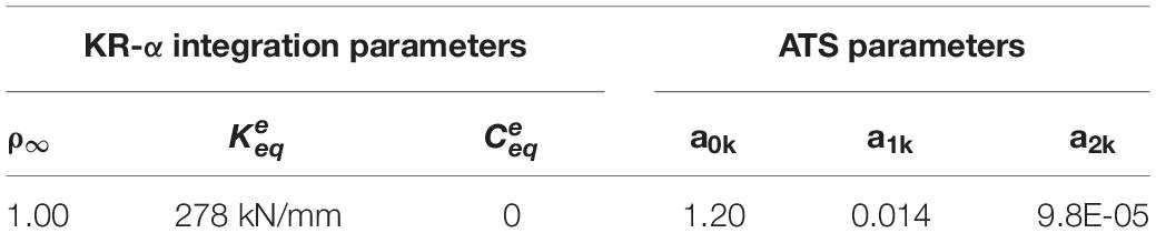
Table 3. Initial parameters for defining KR-α integration and ATS compensator for RTHS tests.

FIGURE 16

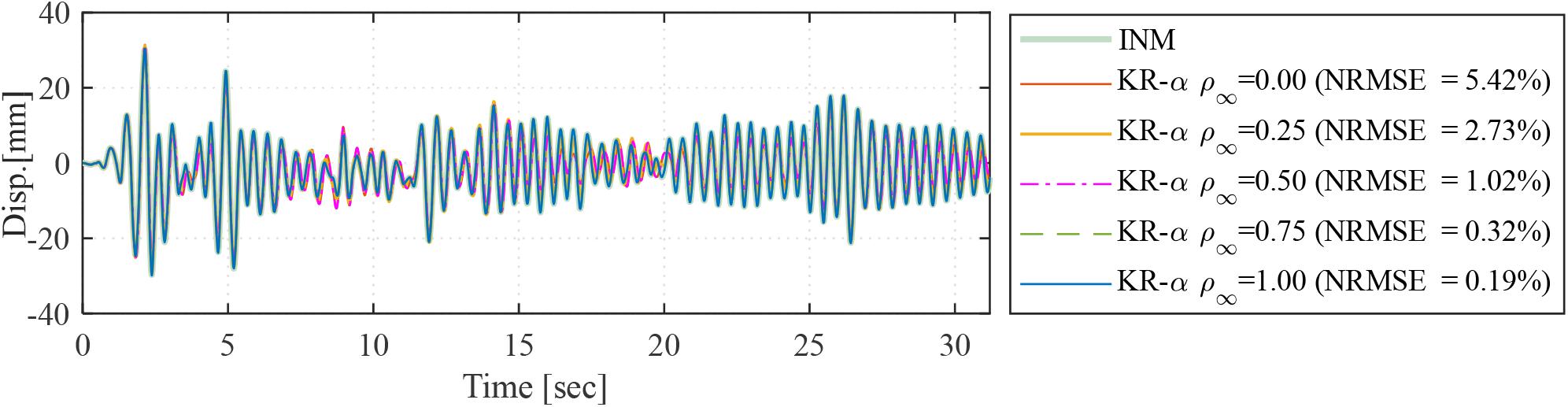
Figure 16. Brace displacement response time histories for different ρ∞ parameter values along with NRMS errors with respect to the implicit Newmark method.

Figure 17 shows the test results from the online RTHS with FE model and without using ATS compensator. Five tests with different geometric scales are shown and compared against the pure analytical solution. Same tests were conducted but with using the ATC actuator delay compensator, and results are shown in Figure 18. For all tests, the obtained brace displacements are shown at the prototype scale so that the different scale tests could be compared. From the figures, it shown that the geometric scale of the experimental substructure, i.e., different range of actuator displacements and velocities, did not affect the test results, which demonstrates the capability of the hydraulic system and actuator. However, it can be clearly seen that the delay of the actuator affected the response in terms of phase difference and amplitude. The ATS is shown to significantly improve the test performance and critically needed for RTHS, which might not be the case when ML models are used in lieu of FE models as discussed in the last section.

FIGURE 17

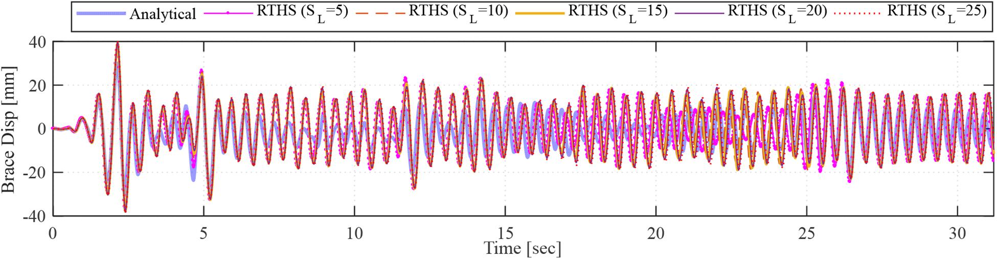
Figure 17. Comparison of brace displacements from online RTHS tests without using ATS compensator (for different geometric scales) against pure analytical solution.

FIGURE 18

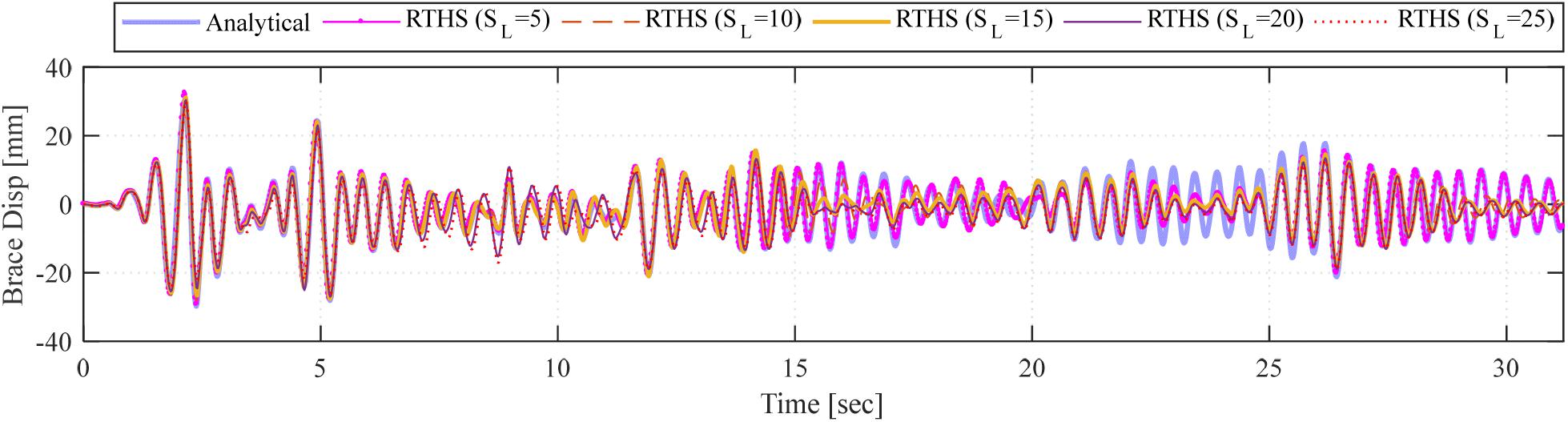
Figure 18. Comparison of brace displacements from online RTHS tests with using ATS compensator (for different geometric scales) against pure analytical solution.

To demonstrate whether the prototype CBF goes non-linear under the 100% scale El Centro ground motion used throughout this study, the force–displacement relationship of the full frame is shown in Figure 19. The figure compares the pure analytical case and one of the online RTHS tests with FE model (with ATS and S_L = 15) as an example. It is shown that even when ATS is used the FE solution for the non-linear model becomes erroneous during online RTHS tests. This error might be attributed to improper estimation of the equivalent initial elastic stiffness or damping matrix for instance. However, such results confirm the need of proper parameters estimation and careful investigation to conduct reliable RTHS tests, which is discussed in detail in Bas and Moustafa (2020). Moreover, to further quantify the performance when non-linear FE model is used for RTHS and to establish a reference case for further ML validations, the NRMSE, NEE, and MAE values were calculated and listed in Table 4. The error values from the cases with and without ATS confirm the importance of using an error compensator for RTHS with FE analytical substructure. The table also confirms that even with ATS, there is still considerable error with respect to the pure analytical solution. Lastly, the error values suggest that system becomes relatively more erroneous at larger geometric scales leading to much smaller actuator displacements.

FIGURE 19

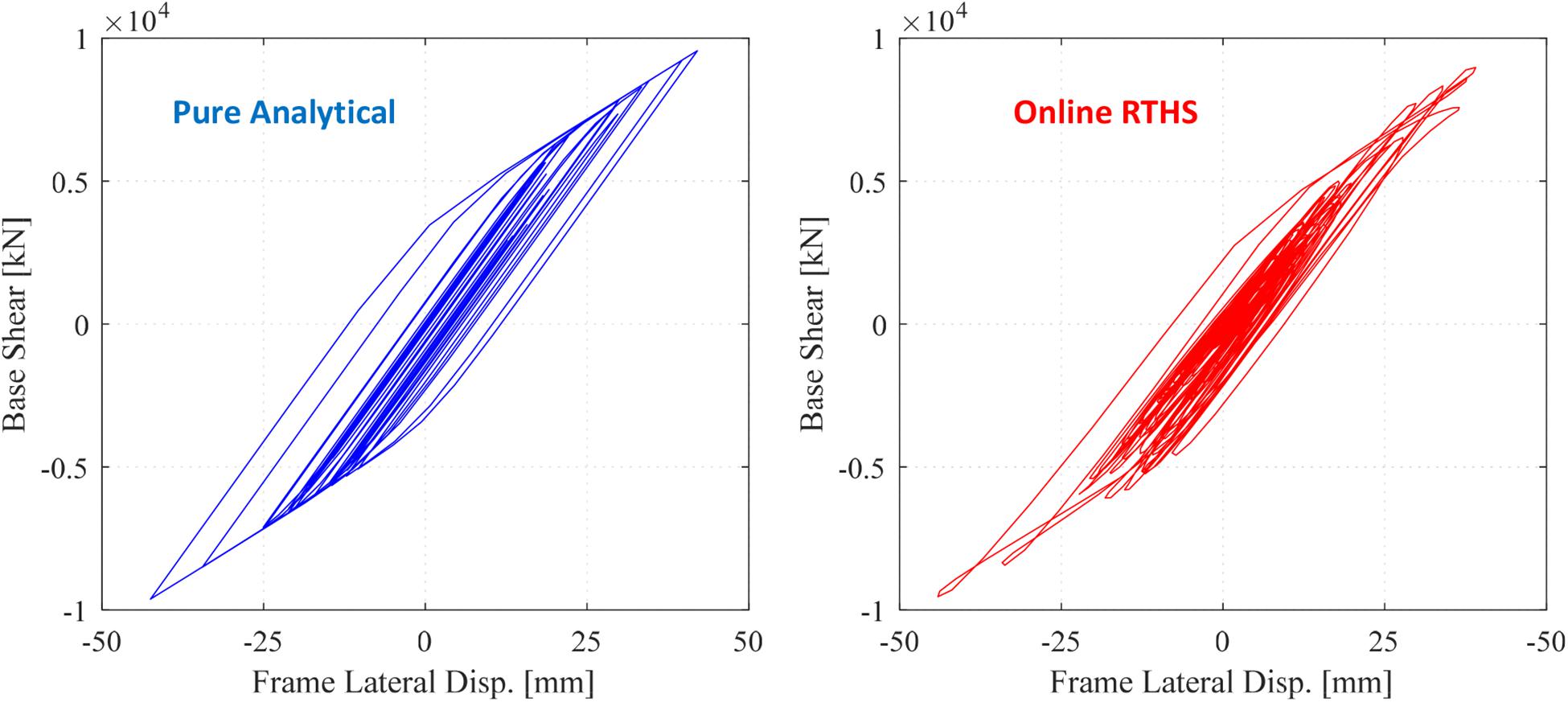
Figure 19. Comparison of global force–displacement relationship for prototype CBF as obtained from pure OpenSees analytical solution and online RTHS with FE model (with ATS and S_L = 15).

TABLE 4

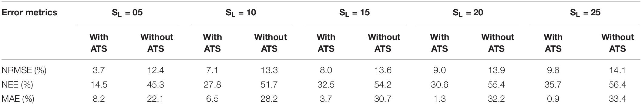
Table 4. Errors (%) in brace displacement response from online RTHS with FE model as compared to the pure analytical solution.

RTHS Testing With ML Models From Local PC and Cluster

As previously mentioned, two ways of running the LSTM ML models have been considered. The data communication is possible when the Python model is run from a high-performance computer or the local computer (i.e., host PC in the UNR setup). In this section, the computational time at each analysis step is presented for both ways of conducting the ML-based RTHS tests. The considered time steps included the time spent for the ML model to evaluate the prediction, i.e., calculation time, the time spent to receive the data from the experimental substructure, and the total data transfer time. It should be noted that the prediction time step and the simulation time step were set to be 0.02 s.

The computational time spent for the online RTHS where Model 1 (with 15 lookbacks) was used as the computational substructure is shown in Figure 20A for the local computer and Figure 20B for the cluster. The average time spent for the ML prediction is estimated to be 10.2 ms for the local PC and 9.4 ms for the cluster. Moreover, the figure shows the overall data transfer time for each analysis step, which is desired to be 20 ms to satisfy the real-time testing through proper OpenFresco handling. It can be seen from Figure 20A that some of the time steps showed minor spikes that took slightly longer than the simulation time step when the tests were conducted from the host PC. However, the total data transfer time remained less than or equal to 20 ms when cluster communication was provided through the SSH network protocol. Figure 21 shows the same comparison when Model 2 with 20 lookbacks was used. The average calculation time for Model 2 was estimated as 11.8 ms for local PC and 10.7 ms for the cluster. It should be noted that Model 2 has a larger dataset dimension (lookback), which slightly increases the prediction time when Models 1 and 2 are compared. Overall, the observations show that the prediction takes slightly less time for cluster than the local computer for both models. For both configurations, the data transmission is done through the UDP channel. However, the UDP channel is provided through SSH network protocol for the cluster, which provides highly stable communication and ensures the desired simulation time step is achieved.

FIGURE 20

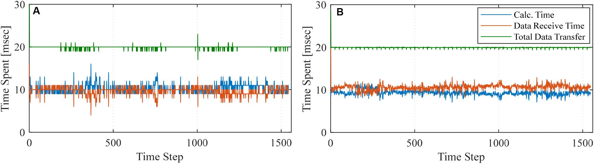
Figure 20. Computational time for RTHS tests with Model 1 located at (A) local PC and (B) cluster.

FIGURE 21

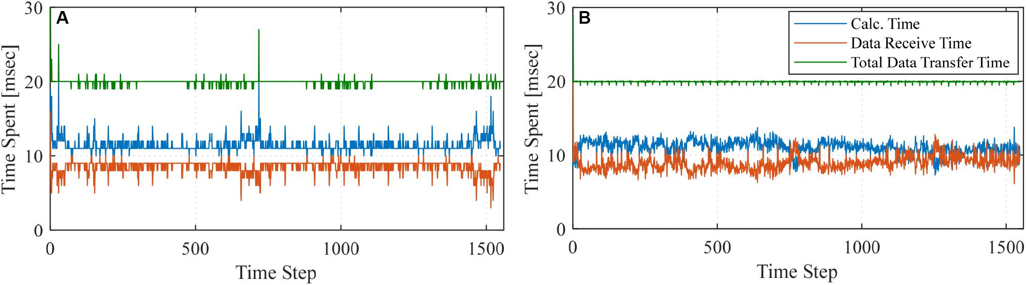
Figure 21. Computational time for RTHS tests with Model 2 located at (A) local PC and (B) cluster.

Validation of RTHS Tests With ML Models and Effect of Delay Compensator

A series of 40 RTHS tests were conducted, which included different ML models and scale factor. The same two advanced LSTM models as before, i.e., Models 1 and 2, were used when located at the local PC, and tests were conducted also at same geometrical scale factors as before, i.e., 5, 10, 15, 20, and 25. Models 1 and 2 were also handled differently to create two more subgroups of models as discussed in the next paragraphs. Additional tests were also conducted using the cluster. However, there was no significant difference in test results when using the local PC and cluster. Therefore, this section only presents the RTHS tests where advanced ML models located and ran from the local PC.

The data shapes of the inputs for Models 1 and 2 are in three dimensions as explained before in Advanced ML Techniques for RTHS. For the RTHS testing, the single value of the force feedback that is obtained from the experimental substructure at each time step is fed into the LSTM model. However, such online value can be used to overwrite, or simply update, one or more of the dimensions of the LSTM lookbacks, i.e., 15 predefined brace force input values, for instance. In this study, two different submodels for both Models 1 and 2 were investigated, which considered two arbitrary dimensions for the update. For first case, the overwritten/updated value was the first row of the 15 or 20 force input lookbacks, which was updated with the online force feedback. The other case considered using the force feedback to update the last row of the lookbacks instead. The two cases are referred to as FIRST and LAST for the remainder of the discussion. For brevity, only few plots from selected RTHS tests are presented, which were obtained for Model 1 with S_L = 15. However, a summary of results from all tests is still provided in terms of error estimation with respect to the pure analytical FE model response.

Figure 22 presents the brace displacement response as adopted from the actuator for RTHS with ML model and with and without using ATS. The figure also compares the RTHS response against the pure analytical solution. The results shown are from a “FIRST”-type case where only the first term on the force input’s lookback dimension was updated with the force feedback obtained from the experimental substructure. The first main and big observation is that RTHS testing with advanced ML model used for non-linear analytical substructure is demonstrated to be a valid approach with very comparable results when compared to analytical solution. The displacement command was predicted well-enough, based on the online received feedback, to conduct the RTHS tests successfully. Results from another test that used the same model but considered the last row of the force input for updating are shown in Figure 23. When the cases with and without ATS are compared in both Figures 22, 23, there is no significant effect on the response. In fact, the feedback that was obtained from the case with ATS was worse and noisier in some cases as in the sample shown in Figure 23, i.e., the actuator became more sensitive to the updated force value when the last term in the lookbacks is overwritten. Nonetheless, even with the added noise in some ML model cases, the response of the actuator remained stable, and the RTHS tests were successfully completed.

FIGURE 22

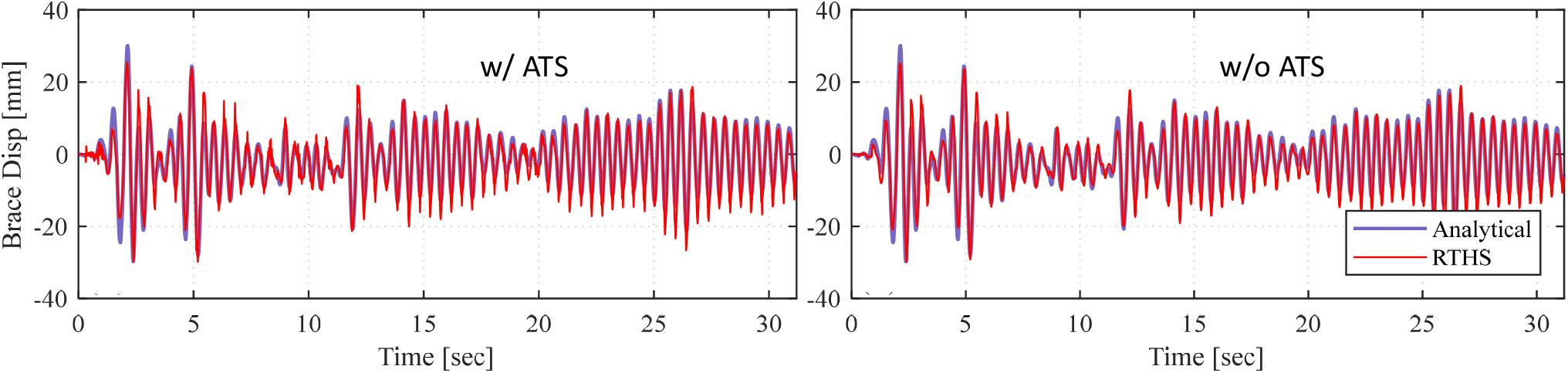
Figure 22. RTHS response comparison with analytical solution for Model 1 (S_L = 15) with and without using ATS when the first row of the force input was selected to be updated.

FIGURE 23

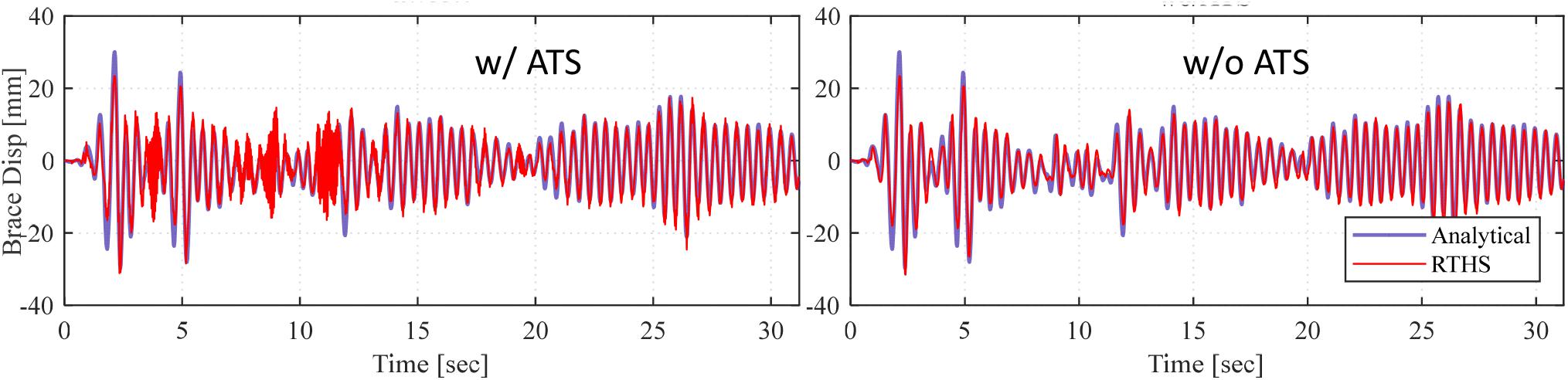
Figure 23. RTHS response comparison with analytical solution for Model 1 (S_L = 15) with and without using ATS when the last row of the force input was selected to be updated.

To comprehensively assess all conducted tests, the NRMSE and NEE values were obtained and summarized in Figure 24 and Table 5. Figure 24 shows the error values for Model 1 for all the RTHS tests with different geometric scales. It can be observed that the effect of the ATS compensator is more pronounced when the last row of the force input is updated with the feedback value from the actuator and at larger-scale factors where smaller actuator displacements were expected. However, this effect of using ATS is even an adverse effect. For instance, using ATS for the case with S_L = 25 led to dramatic increase in error value. Regardless of the ATS effect, it is shown that ML models do not need to be used with actuator delay compensation because of the nature of the model training that indirectly accommodates actuator delays. This preliminary observation is worth further investigation where ML models could be considered to improve actuator control in cases of non-linear dynamic systems.

FIGURE 24

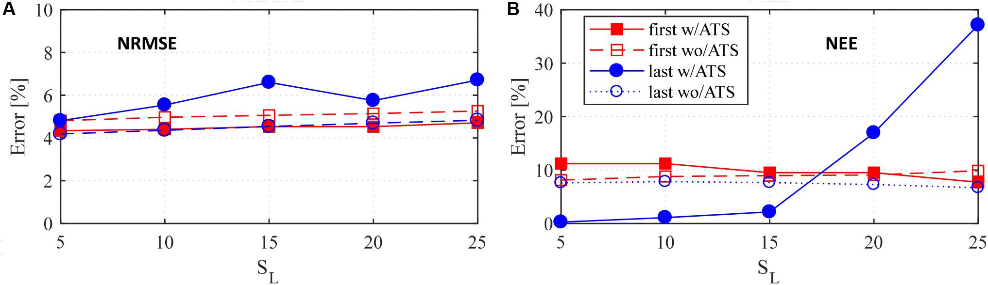
Figure 24. RTHS (A) NRMSE and (B) NEE calculation for Model 1 (all geometric scales).

TABLE 5

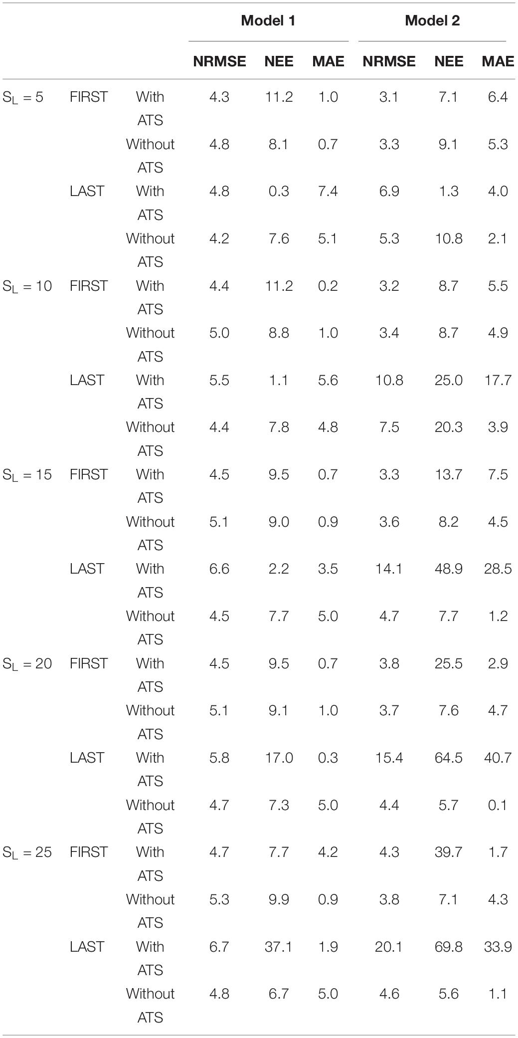
Table 5. Error estimation (%) for all conducted online RTHS tests with different ML models with respect to the pure analytical solution.

Table 5 presents all the error metrics for 40 different RTHS tests with ML models located at host PC. Detailed evaluations for Models 1 and 2 are reported in terms of NRMSE, NEE, and MAE. All RTHS tests were successfully completed for each model and geometric scale factor. In most cases, the RMSE is less than 5%, which is reasonably accurate to confidently validate the proposed concept of using ML models to replace FE models within the RTHS loop. Moreover, Models 1 and 2 do not show any significant differences for most of the considered tests. It is observed that the most problematic cases were observed when the last row of the force input was updated, and larger geometric scales were used with the ATS compensator. However, even for these cases, the tests remained stable, and none of the tests were stopped unlike what was previously reported for using non-linear FE models (Bas and Moustafa, 2020). The results are encouraging in terms of eliminating the need for any delay compensator when ML models are used for RTHS. In summary, this study sets the stage for a new way of conducting RTHS testing in the future. However, the results also show that the hardware, geometric scale, and type of ML model could have significant effect on accuracy of RTHS testing and justify the call for further research studies to identify best ML practices and modeling procedures for future RTHS testing.

Summary and Conclusion

In this article, the idea of using complex ML models to replace FE models for RTHS was validated, and foundational work was provided for RTHS communication development and verification for Python-based deep learning ML metamodels. This study was motivated by the potential for ML-based computational substructures to advance RTHS testing and help explore new research areas in the future. The article touches on ML models sensitivity and performance for time-series prediction, as well as using high-performance computers for running online ML models. The need for commonly used practices in RTHS testing, e.g., actuator delay compensation, was also assessed when ML metamodels are used for the computational substructures. For all ML models and system evaluations, a one-bay, one-story steel braced frame was selected. The columns and beam defined the analytical substructure, whereas the brace defined the experimental substructure for RTHS testing. The key aspects of the study along with the main findings can be summarized as follows.

• A simplified ML model was first generated with LR algorithms for a linear elastic system. The LR model was coded using MATLAB/Simulink and compiled on the xPC machine as part of the RTHS loop. No specific communication scheme was needed, and the simple tests showed that using metamodels to derive the actuator in an RTHS setting is possible.

• For accurate modeling of dynamic response of non-linear braced frames, LR models could not be used, and more advanced ML algorithms were needed. Deep LSTM networks were selected because of their capability of capturing long-term patterns in time series. Python was used to generate the LSTM models using training datasets obtained from analytical OpenSees models. A linear elastic brace was considered along with the non-linear frame, and several ML models were evaluated against the pure analytical FE model response to tune the hyperparameters of the model. Two LSTM metamodels were demonstrated to accurately predict non-linear response and in turn, selected to be used further in the RTHS tests.

• The training domain is crucial and should be devised carefully for a robust ML model. In this study, in order to consider the uncertainties due to force–displacement dependencies and hardware errors (e.g., initial load frame feedback, noise from actuator, etc.), the training domain was expanded using seven episodes of the force input to the LSTM model with introduced bias. Although this approach helped, there is need to devise other different training approaches in future studies to account for wide range of uncertainties.

• In order to use Python as a computational driver for ML-based RTHS tests, a communication scheme that uses OpenFresco was proposed and successfully verified. OpenFresco serves a middle-tier server, and Python is the client in this form of architecture. The data transfer is made through UDP socket between Python and OpenFresco. Data communication from both local PC and high-performance computer cluster was verified. The cluster communication is achieved through UDP socket but under the secure shell portal.

• When comparing the use of local PC versus cluster for running online RTHS Python LSTM models, no significant improvement in computational time is observed for the considered CBF structure. However, it is reported that using the cluster through the secure shell network protocol provides more stable communication than local PC where no data transfer time spikes were observed. The data transfer time for each analysis step was always guaranteed to be equal to or less than the defined simulation time step when the cluster was used.

• Several RTHSs were successfully conducted, and their results were used to assess the performance of the developed communication, as well as the python-based deep LSTM model validity. Several RTHS tests were conducted using non-linear FE to better assess the benefits of the ML modeling approach. It was shown that FE models, in case of non-linearity, could result in relatively more errors and is much more dependent on actuator delay compensators when compared to ML models.

• The preliminary results presented in this study suggest that a dedicated actuator delay compensator might not be needed. Instead, such compensation can be embedded within the ML model, which works with recurrent data, and considered a priori as part of the training. While sufficient evidence and verification are still needed, this observation is worth further investigation to explore the use of ML models to improve actuator control in cases of non-linear dynamic systems.

• Overall, the communication developments for RTHS tests with advanced Python-based ML models are successfully validated for the first time. The goal of the article was not necessarily to present most the accurate or exact ML models for a given non-linear analytical substructure, but rather to demonstrate the concept of using ML algorithms within the HS loop. The study shows the applicability of using robust clusters and calls for future research to consider supercomputers, clusters with GPU, etc., for running ML models for RTHS. One main limitation in this study is not using realistic or non-linear experimental substructures. Thus, future work is recommended to consider new ML methods that can be trained for non-linear specimen response.

Data Availability Statement

The raw data supporting the conclusions of this article will be made available by the authors, without undue reservation.

Author Contributions

EB: system development, testing, data collection and analysis, data and results interpretation, and writing original manuscript. MM: conceptualization, data and results interpretation, reviewing and editing manuscript, and project supervising. Both authors contributed to the article and approved the submitted version.

Conflict of Interest

The authors declare that the research was conducted in the absence of any commercial or financial relationships that could be construed as a potential conflict of interest.

References

Abadi, M., Ashish, A., Paul, B., Eugene, B., Zhifeng, C., Craig, C., et al. (2015). TensorFlow: Large-Scale Machine Learning on Heterogeneous Distributed Systems. Available online at: http://arxiv.org/abs/1603.04467 (accessed June 3, 2020).

Google Scholar

Abbiati, G., Lanese, I., Cazzador, E., Bursi, O. S., and Pavese, A. (2019). A computational framework for fast-time hybrid simulation based on partitioned time integration and state-space modeling. Struct. Contr. Health Monit. 26, 1–28. doi: 10.1002/stc.2419

CrossRef Full Text | Google Scholar

Ahmadizadeh, M., Gilberto, M., and Andrei, M. R. (2008). Compensation of actuator delay and dynamics for real-time hybrid structural simulation. Earthquake Engin. Struct. Dynam. 37, 21–42. doi: 10.1002/eqe.743

CrossRef Full Text | Google Scholar

Bas, E. E., and Moustafa, A. M. (2020). Performance and limitations of real-time hybrid simulation with nonlinear computational subsructures. Exper. Techniq. 2020, 121. doi: 10.1007/s40799-020-00385-6

CrossRef Full Text | Google Scholar

Bas, E. E., Moustafa, M. A., Feil-Seifer, D., and Blankenburg, J. (2020a). Using machine learning approach for computational substructure in real-time hybrid simulation. arXiv 2004:02037.

Google Scholar

Bas, E. E., Mohamed, A. M., and Gokhan, P. (2020b). Compact hybrid simulation system: validation and applications for braced frames seismic testing. J. Earthqu. Engin. 2020, 1–30. doi: 10.1080/13632469.2020.1733138

CrossRef Full Text | Google Scholar

Bengio, Y., Patrice, S., and Paolo, F. (1994). Learning long-term dependencies with gradient descent is difficult. IEEE Transac. Neur. Net. 5, 157–166. doi: 10.1109/72.279181

CrossRef Full Text | Google Scholar

Bonelli, A., and Bursi, S. O. (2005). Predictor-corrector procedures for pseudo-dynamic tests. Engin. Comput. 22, 783–834. doi: 10.1108/02644400510619530

CrossRef Full Text | Google Scholar

Carrion, J. E., and Spencer, B. F. (2007). Model-Based Strategies for Real-Time Hybrid Testing. NSEL Report No. NSEL-006 India: Indian Institute Of Technology.

Google Scholar

Chae, Y., Karim, K., and James, M. R. (2013). Adaptive time series compansator for delay compensation of servo-hydraulic actuator systems for real-time hybrid simulation. Earthquake Engin. Struct. Dynam. 42, 1697–1715. doi: 10.1002/eqe.2294

CrossRef Full Text | Google Scholar

Chang, S.-Y. (2002). Explicit pseudodynamic algorithm with unconditional stability. J. Engin. Mechan. 128, 935–947. doi: 10.1061/(ASCE)0733-9399(2002)128:9(935)

CrossRef Full Text | Google Scholar

Chang, S.-Y. (2009). An explicit method with improved stability property. Int. J. Num. Method. Engin. 77, 1100–1120. doi: 10.1002/nme.2452

CrossRef Full Text | Google Scholar

Chen, C., and Ricles, J. M. (2010). Tracking error-based servohydraulic actuator adaptive compensation for real-time hybrid simulation. J. Struct. Engin. 136, 432–440. doi: 10.1061/(ASCE)ST.1943-541X.0000124

PubMed Abstract | CrossRef Full Text | Google Scholar

Chen, C., Ricles, J. M., Marullo, T. M., and Mercan, O. (2009). Real-time hybrid testing using the unconditionally stable explicit CR integration algorithm. Earthquake Engin. Struct. Dynam. 38, 23–44. doi: 10.1002/eqe.838

CrossRef Full Text | Google Scholar

Chollet, F. (2015). Keras: Deep Learning Library for Theano and Tensorflow. Available online at: https://keras.io/k (accessed June 3, 2020).

Google Scholar

Darby, A. P., Williams, M. S., and Blakeborough, A. (2002). Stability and delay compensation for real-time substructure testing. J. Engin. Mechan. 128, 1276–1284. doi: 10.1061/(ASCE)0733-93992002128:121276

CrossRef Full Text | Google Scholar

Del Carpio, M., Hashemi, M. J., and Mosqueda, G. (2017). Evaluation of integration methods for hybrid simulation of complex structural systems through collapse. Earthquake Engin. Vibr. 16, 745–759. doi: 10.1007/s11803-017-0411-z

CrossRef Full Text | Google Scholar

Filippou, F. C., Popov, E. P., and Bertero, V. V. (1983). Effects of Bond Deteroriation on Hysteretic Behavior of Reinforced Concrete Joints. Report No. UCB/EERC-83/19 California, CA: UCB.

Google Scholar

Géron, A. (2017). Hands-on Machine Learning with Scikit-Learn and TensorFlow. Massachusetts: O’Reilly Media, Inc.

Google Scholar

Hochreiter, S., and Jürgen, S. (1997). Long short-term memory. Neur. Comput. 9, 1735–1780. doi: 10.1162/neco.1997.9.8.1735

PubMed Abstract | CrossRef Full Text | Google Scholar

Jozefowicz, R., Wojciech, Z., and Ilya, S. (2015). “An empirical exploration of recurrent network architectures,” in Proceedings of the 32nd International Conference on Machine Learning (France: ICML).

Google Scholar

Kingma, D. P., and Ba, L. J. (2015). “Adam: a method for stochastic optimization,” in 3rd International Conference on Learning Representations, ICLR 2015 - Conference Track Proceedings (France: ICML), 1–15.

Google Scholar

Kolay, C., James, M. R., Marullo, T. M., Mashvashmohammadi, A., and Sause, R. (2015). Implementation and application of the unconditionally stable explicit parametrically dissipative KR-Alpha method for real-time hybrid simulation. Earthquake Engin. Struct. Dynam. 44, 735–755. doi: 10.1002/eqe.2484

CrossRef Full Text | Google Scholar

Kolay, C., and Ricles, M. J. (2014). Development of a family of unconditionally stable explicit direct integration algorithms with controllable numerical energy dissipation. Earthquake Engin. Struct. Dynam. 43, 1361–1380. doi: 10.1002/eqe

CrossRef Full Text | Google Scholar

Lagaros, N. D., and Manolis, P. (2012). Neural network based prediction schemes of the non-linear seismic response of 3D buildings. Adv. Engin. Soft. 44, 92–115. doi: 10.1016/j.advengsoft.2011.05.033

CrossRef Full Text | Google Scholar

LeCun, Y., and Yoshua, B. (1995). “Convolutional networks for images, speech, and time-series,” in The Handbook of Brain Theory and Neural Networks, ed. M. A. Arbib (Cambridge: MIT Press), 255–258.

Google Scholar

Mai, C. V., Spiridonakos, M. D., Chatzi, E. N., and Sudret, B. (2016). Surrogate modelling for stochastic dynamical systems by combining NARX models and polynomial chaos expansions. arXiv 1604.07627.

Google Scholar

McKenna, F., Fenves, G. L., and Scott, M. H. (2000). Open System for Earthquake Engineering Simulation Pacific Earthquake Engineering Research Center. Belgium: PEER.

Google Scholar

Miraglia, G., Petrovic, M., Abbiati, G., Mojsilovic, N., and Stojadinovic, B. (2020). A model-order reduction framework for hybrid simulation based on component-mode synthesis. Earthquake Engin. Struct. Dynam. 49, 737–753. doi: 10.1002/eqe.3262

CrossRef Full Text | Google Scholar

Moustafa, M. A., and Mosalam, K. M. (2015a). “Development of hybrid simulation system for multi-degree-of-freedom large-scale testing,” in 6th International Conference on Advances in Experimental Structural Engineering (Urbana: University of Illinois).

Google Scholar

Moustafa, M. A., and Mosalam, K. M. (2015b). Structural Behavior of Column-Bent Cap Beam-Box Girder Systems in Reinforced Concrete Bridges Subjected to Gravity and Seismic Loads Part II: Hybrid Simulation and Post-Test Analysis. California: University of California, Berkeley.

Google Scholar

Mucha, W. (2019). Application of artificial neural networks in hybrid simulation. Appl. Sci. 9:4495. doi: 10.3390/app9214495

CrossRef Full Text | Google Scholar

Phillips, B. M., and Spencer, B. F. (2013). Model-based feedforward-feedback actuator control for real-time hybrid simulation. J. Struct. Engin. 139, 1205–1214. doi: 10.1061/(ASCE)ST.1943-541X.0000606

PubMed Abstract | CrossRef Full Text | Google Scholar

Schellenberg, A. H., Kim, H. K., and Mahin, S. A. (2009a). OpenFresco. California: Universtiy of California, Berkeley.

Google Scholar

Schellenberg, A. H., Mahin, S. A., and Fenves, G. L. (2009b). Advanced Implementation of Hybrid Simulation. Report No. PEER 2009/104 California: Berkeley.

Google Scholar

Schellenberg, A., Kim, H. K., Fenves, G. L., and Mahin, S. A. (2009c). OpenFresco Framework for Hybrid Simulation: Simulation Finite Element Adapter Experimental Control Example. Engineering Simulation. California: Berkeley.

Google Scholar

Schellenberg, A., Kim, H. K., Takahashi, Y., Fenves, G. L., and Mahin, S. A. (2009d). OpenFresco Command Language Manual. California: Berkeley.

Google Scholar

Serebanha, A., Schellenberg, A. H., Schoettler, M. J., Mosqueda, G., and Mahin, S. A. (2019). Real-time hybrid simulation of seismically isolated structures with full-scale bearings and large computational models. CMES 120, 693–717. doi: 10.32604/cmes.2019.04846

CrossRef Full Text | Google Scholar

Takanashi, K., Udagawa, K., Seki, M., Okada, T., and Tanaka, H. (1975). Non-linear earthquake response analysis of structures by a computer-actuator on-line system. Transac. Arch. Instit. J. 229, 77–83. doi: 10.3130/aijsaxx.229.0_77

CrossRef Full Text | Google Scholar

Wallace, M. I., Wagg, D. J., and Neild, S. A. (2005). An adaptive polynomial based forward prediction algorithm for multi-actuator real-time dynamic substructuring. Proc. Roy. Soc. A Math., Phys. Engin. Sci. 461, 3807–3826. doi: 10.1098/rspa.2005.1532

Google Scholar

Wang, Y., Chong, W., Hui, L., and Zhao, R. (2009). “Artificial neural network prediction for seismic response of bridge structure,” in 2009 International Conference on Artificial Intelligence and Computational Intelligence AICI 2009, Vol. 2, (Berlin: Springer), 503–506.

Google Scholar

Xie, Y., Sichani, M. E., Padgett, J. E., and DesRoches, R. (2020). The promise of implementing machine learning in earthquake engineering: a state-of-the-art review. Earthquake Spectra 2020, 1–33. doi: 10.1177/8755293020919419

CrossRef Full Text | Google Scholar

Zhang, R., Liu, Y., and Sun, H. (2019a). Physics-guided convolutional neural network (PhyCNN) for data-driven seismic response modeling. arXiv 216:110604.

Google Scholar

Zhang, R., Zhao, C., Chen, S., Zheng, J., Büyüköztürk, O., and Sun, H. (2019b). Deep long short-term memory networks for nonlinear structural seismic response prediction. Comput. Struct. 220, 55–68. doi: 10.1016/j.compstruc.2019.05.006

CrossRef Full Text | Google Scholar

Zhao, J., French, C., Shield, C., and Posbergh, T. (2003). Considerations for the development of real-time dynamic testing using servo-hydraulic actuation. Earthquake Engin. Struct. Dynam. 32, 1773–1794. doi: 10.1002/eqe.301

CrossRef Full Text | Google Scholar