An Examination of the Gust Effect Factor for Rigid High-Rise Buildings

Introduction

The gustiness in wind can be regarded as a combination of eddies of different sizes (Greenway, 1979; Holmes, 2015). For rigid buildings, it is assumed that maximum wind loads acting on the entire structure are caused by well-correlated gusts that envelope the entire structure. For flexible buildings, these wind gusts can introduce dynamic oscillations of the structure, such that maximum loads should also include these load effects. For loads on building components and cladding, maximum loads occur through a combination of the well-correlated large-scale gusts with the smaller scale eddies in the wind and those generated by the building.

For the wind design process, the effects of the wind gusts and structural dynamics are usually characterized by an amplification factor called the gust-response or gust-loading factor. The gust response factor is defined as the ratio of expected maximum response of the structure to the mean response (Holmes, 2015). The concept provides a straightforward approach to estimate the equivalent static wind loads, i.e., the loads that when statically applied to the building will cause the same maximum response (Kareem and Zhou, 2003).

The concept and formulation of the gust loading factor was first proposed by Davenport (1967), but has been further advanced by many scholars (Vickery 1970; Simiu, 1977; Solari 1993a, 1993b; Zhou et al., 1999; Zhou and Kareem, 2001; Piccardo and Solari, 2002). Among them, Solari (1993a, 1993b) developed a general procedure for treating the gust buffeting problem in a unified way, and derived the solutions for peak wind velocity, equivalent pressure on rigid buildings, and the dynamic along-wind response of buildings in a closed form. Zhou et al. (1999), Zhou and Kareem. (2001) developed a more realistic design procedure using the base moment gust loading factor, which can estimate base shears more accurately compared to a displacement gust loading factor. Piccardo and Solari (2002) developed a closed-form solution of the 3-D gust loading factor for uncoupled along-wind, cross-wind and torsional wind-excited responses. Although different formulations of the gust loading factor have been advanced, derivations of the formulations in these studies follow the same framework using a spectral approach with calculations based primarily in the frequency domain (Davenport, 1963; Holmes, 2015). Starting from the wind velocity spectrum, the aerodynamic force spectrum can be obtained by introducing the aerodynamic admittance function (AAF) with the velocity spectrum, based on the quasi-steady theory (Stathopoulos, 1983; Solari, 1993a; Holmes, 2015; Wu and Kopp, 2016). Then, the response spectrum can be obtained by introducing the mechanical admittance to the force spectrum, based on random vibration theory (Holmes, 2015). Finally, the gust loading factor can be calculated using the mean square fluctuating response and a Gaussian peak factor, which are obtained from the integration of the response spectrum and the method developed by Davenport (Davenport, 1964), respectively.

For rigid buildings, the problem becomes relatively simpler, as the structural dynamics are not considered, i.e., the spectral approach only needs to proceed to the step of determining the force spectrum. For this case, only the background response component in the gust loading factor is considered, while the resonant response is neglected. Thus, the equivalent static wind loads reduce to the maximum (peak) wind loads. The remainder of this paper focuses solely on these aerodynamic loads.

Due to instrumentation limitations at the time that these methods were developed, rational peak loads were obtained theoretically from the easier-to-obtain mean loads. However, in this process, many assumptions and approximations were made. For example, the quasi-static assumption, where the fluctuating pressure on a structure follows the variations of upstream wind velocity (squared), is usually the basis for most derivations of peak loads. Based on the quasi-static assumption, the link between the force spectrum and velocity spectrum, (i.e. the AAF) in the above literature usually only includes the spatial correlation of wind speeds. This means that only the effects of non-contemporaneous gust actions over the structure are considered, while the effects of body-generated turbulence are ignored. This may result in certain deviations of the estimated peak values from the true peaks. In addition, based on the quasi-static assumption, the fluctuating pressures are assumed to constitute a Gaussian process following the longitudinal fluctuating wind speed so that a Gaussian peak factor method can be the applied.

The shortcomings of the theoretical approach can be compensated for by experimental approaches, especially with the advances in measurement instrumentation. It is now common to obtain peak values through a combination of accurate measurements and an appropriate extreme value analysis. As well, the distinct approaches to obtain peak loads (gust response factor applied to mean load vs. directly measured peaks) have emerged because the former needs to consider how to rationally include the structural dynamic loads while the latter is usually applied to non-resonant structures. This distinction could also be written as one between the approaches used in design provisions for high-rise buildings (which often need to consider structural dynamics in design) and low-rise buildings (which are usually considered non-resonant). This has played out in ASCE 7 with two distinct methods for determining design loads: 1) Chapter 27, which applies to buildings of all heights, including low-rise buildings, using the gust effect factor approach, and 2) Chapter 28, which only applies to low-rise buildings, uses directly obtained peak loads. These two approaches lead to different design wind loads, which is perhaps unsurprising. The current paper focuses on the role of the gust effect factor in such differences.

In our previous work (Liu et al., 2019), we show that for a series of wind tunnel tests on high-rise buildings, the measured gust effect factor for rigid buildings is significantly higher than in Chapter 27 of ASCE 7–16 for certain cases. In light of this, the objective of this paper is to systematically investigate the gust effect factor in order to determine what is causing this difference. Ultimately, we expect that this could improve the consistency between Chapters 27 and 28 of ASCE 7–16 by developing an improved understanding of the aspects that effect the calculation of peak values via the gust effect factor (Chapter 27) compared to directly measured peak values (Chapter 28). In order to achieve the objective, the derivation of the gust effect factor in ASCE 7–16 is reviewed and examined in detail with recently obtained experimental data from (Liu et al., 2019).

Gust Effect Factor in ASCE 7

Due to the relative simplicity and effectiveness of the gust loading factor method, it has been employed in most wind loading provisions and standards (Kijewski and Kareem, 1998; Zhou et al., 2002; Kareem and Zhou, 2003). ASCE 7–16 (2016) also uses this method, which is mainly based on (Solari, 1993a; 1993b). In order to assess the effects of various assumptions, the derivation of the ASCE 7 gust effect factor for rigid buildings is reviewed in this section.

In ASCE 7–16 (2016), the design wind pressures for the MWFRS of buildings are given by:

$p={\widehat{q}}_{z}G{\overline{C}}_p,(1)$

where p is the equivalent static wind pressure, ${\widehat{q}}_z$ is the peak dynamic pressure, ${\overline{C}}_p$ is the mean pressure coefficient, and G is the gust effect factor. According to Solari and Kareem (1998), the gust effect factor, G, is the gust response factor, G_Y, divided by the gust pressure factor, G_P:

$G=\frac{G_Y}{G_P},(2)$

where G_P is a conversion factor for the dynamic wind pressure from the mean wind speed to the peak wind speed. The 3 s gust wind speed is the basic wind speed in ASCE 7–16. For rigid buildings, the structural dynamics are not considered. In this case, the equivalent static wind pressure is the peak wind pressure, and the gust response factor G_Y in Eq. 2 can be replaced by G_Q, where G_Q is the gust response factor for rigid buildings. This can also be called the gust equivalent pressure factor. Thus, for rigid buildings, Eq. 2 can be written as:

$G=\frac{G_Q}{G_P}.(3)$

Gust Pressure Factor

In the ASCE 7–16 formulations of both the gust pressure factor, G_P, and gust response factor G_Q, Davenport’s method (Davenport, 1964; Solari, 1993a) for estimating instantaneous maxima has been employed. For a stochastic stationary Gaussian process, $E=\overline{E}+e$, where $\overline{E}$ is the time-averaged mean value of E and $e$ is the zero mean fluctuation, the expected instantaneous maximum value, $\widehat{E}$, can be obtained from:

$\widehat{E}=\overline{E}+g_e{\sigma }_e=G_e\overline{E},(4)$

where G_e is the gust factor and g_e is the peak factor, which can be calculated, assuming a stationary Gaussian process, by:

$g_e=\sqrt{2\ln \left[v_{e}T\right]}+\frac{0.5772}{\sqrt{2\ln \left[v_{e}T\right]}}\cong {\left\{1.175+2\ln \left[v_{e}T\right]\right\}}^{1/2},(5)$

$G_E=1+g_e\frac{{\sigma }_e}{\overline{E}},(6)$

$v_e=\frac{1}{2\pi }\frac{{\sigma }_{\dot{e}}}{{\sigma }_e},(7)$

${\sigma }_e^2={\displaystyle {\int }_0^{\infty }{S}_e\left(f\right)}\text{d}f,(8)$

${\sigma }_{\dot{e}}^2={\displaystyle {\int }_0^{\infty }{\left(2\pi f\right)}^2{S}_e\left(f\right)}\text{d}f,(9)$

where σ_e and S_e are the standard deviation and power spectral density of e, respectively, and f is the frequency.

The longitudinal wind velocity can be regarded as a stochastic Gaussian variable. Thus, applying the above method, the gust velocity factor G_U can be obtained by:

$G_U=1+g_u{I}_u\sqrt{P_0},(10)$

$g_u\cong {\left\{1.175+2\ln \left[\tilde{T}\sqrt{\frac{P_1}{P_0}}\right]\right\}}^{1/2},(11)$

$P_0={\displaystyle {\int }_0^{\infty }\frac{S_u\left(f\right)}{{\sigma }_u^2}X\left(f,\tau \right)}\text{d}f,(12)$

$P_1={\displaystyle {\int }_0^{\infty }{\left[\frac{f{L}_u}{\overline{U}}\right]}^2\frac{S_u\left(f\right)}{{\sigma }_u^2}}X\left(f,\tau \right)\text{d}f,(13)$

$\tilde{T}=\frac{T\overline{U}}{L_u},(14)$

$X\left(f,\tau \right)=\frac{{\sin }^2\left(\pi f\tau \right)}{{\left(\pi f\tau \right)}^2},(15)$

where τ is the averaging time of the peak gust and T is duration over which the wind speed is averaged. In ASCE 7, τ = 3 s and T = 1 h; $\overline{U}$ is the mean wind speed, σ_u is the rms (root-mean-square) of the fluctuating wind speed, $I_u$ is the turbulence intensity, $L_u$ is the integral length scale and S_u is the longitudinal velocity power spectral density; X (f, τ) is a τ s moving average filter (Kwon and Kareem, 2014). Following the quasi-steady assumption, the gust pressure factor G_P can be obtained by:

$G_P=\frac{0.5\rho {\widehat{U}}^2}{0.5\rho {\overline{U}}^2}=G_U^2\cong 1+2g_u{I}_u\sqrt{P_0}.(16)$

Gust Response Factor for Rigid Buildings

When estimating the peak wind loads on a rigid building of finite surface area, (i.e. neglecting the resonant response), the correlation of fluctuating wind velocity must be taken into consideration. The imperfect spatial correlation of the upstream wind speed will result in non-contemporaneous gust actions over the entire building surface, reducing the overall peak load compared to directly integrating point peak loads. In simple terms, the peak pressures do not occur simultaneously at every location on the surface. Solari considered this effect by using the equivalent wind spectrum technique (Solari, 1988; Solari, 1993a). Following Solari’s derivation, the gust response factor for rigid buildings, G_Q, can be calculated by:

$G_Q=1+2g_q{I}_u\sqrt{Q_0},(17)$

$g_q\cong {\left\{1.175+2\ln \left[\tilde{T}\sqrt{\frac{Q_1}{Q_0}}\right]\right\}}^{1/2},(18)$

$Q_0={\displaystyle {\int }_0^{\infty }\frac{S_u\left(f\right)}{{\sigma }_u^2}x\left(f\right)X\left(f,\tau \right)}\text{d}f,(19)$

$Q_1={\displaystyle {\int }_0^{\infty }{\left[\frac{f{L}_u}{\overline{U}}\right]}^2\frac{S_u\left(f\right)}{{\sigma }_u^2}}x\left(f\right)X\left(f,\tau \right)\text{d}f,(20)$

$x\left(f\right)=l\left\{\frac{0.4f{C}_{x}B}{{\overline{U}}_h}\right\}l\left\{\frac{0.4f{C}_{z}H}{{\overline{U}}_h}\right\},(21)$

$l\left(\eta \right)=\frac{1}{\eta }-\frac{1}{2{\eta }^2}\left(1-e^{-2\eta }\right),(22)$

where B and H are breadth and height of the building, respectively, h is the reference height, usually h = 0.6H; $C_x$ and $C_z$ are exponential decay coefficients; x(f) was obtained by considering the spatial coherence of wind gusts (Solari, 1988).

Substituting Eqs 16, 17 into Eq. 3, the gust effect factor can be expressed as:

$G=\frac{1+2g_q{I}_u\sqrt{Q_0}}{1+2g_u{I}_u\sqrt{P_0}}.(23)$

It is important to note that, the term x(f) has been introduced into Q₀ and Q₁ (in Eqs 19, 20) in order to describe the effects of imperfect correlations of fluctuating pressures over the building surface. For a structure with a finite surface, the introduction of x(f) will result in a lower value of the numerator compared to the denominator, (i.e. G_Q and G_P, respectively, see Eq. 3); thus, G may have a value less than unity for rigid buildings (with this model). The factor, x(f), modifies the wind spectrum to obtain an effective pressure spectrum considering the spatial extent of the building. In other words, it acts much like the aerodynamic admittance, as discussed further below.

Parametric Analysis of Gust Effect Factor

Based on the model for the turbulence, the following approximations for variables P₀, P₁, Q₀ and Q₁ were made by Solari (1993a):

$P_0=\frac{1}{1+0.56{\tilde{\tau }}^{0.74}},(24)$

$\frac{P_1}{P_0}=\frac{1}{31.25{\tilde{\tau }}^{1.44}},(25)$

$Q_0=\frac{1}{1+0.56{\tilde{\tau }}^{0.74}+0.29{\tilde{L}}_0^{0.63}},(26)$

$\frac{Q_1}{Q_0}=\frac{1}{31.25{\tilde{\tau }}^{1.44}+1.23{\tilde{L}}_1^{1.23}},(27)$

where:

${\tilde{L}}_0=0.42\left(\tilde{B}+\tilde{H}\right)+0.16\sqrt{\tilde{B}\tilde{H}},(28)$

${\tilde{L}}_1=0.04\left(\tilde{B}+\tilde{H}\right)+0.92\sqrt{\tilde{B}\tilde{H}},(29)$

$\tilde{B}=\frac{C_{x}B}{L_{uh}},\tilde{H}=\frac{C_{z}H}{L_{uh}},(30)$

$\tilde{\tau }=\frac{\tau \overline{U}}{L_u},(31)$

Substituting Eqs 24, 26 into Eq. 23 and rearranging yields:

$\begin{array}{l}G=\frac{1+2g_q{I}_u\sqrt{P_0}{Q}_u}{1+2g_u{I}_u\sqrt{P_0}},\\ {\sigma }_u^2=\frac{Q_0}{P_0}=\frac{1+0.56{\tilde{\tau }}^{0.74}}{1+0.56{\tilde{\tau }}^{0.74}+0.29{\tilde{L}}_0^{0.63}}.\end{array}(32)$

According to Solari and Kareem (1998), $\overline{U}/L_u$ usually falls in the range of 0.1–0.3 s⁻¹. Using an average value of $\overline{U}/L_u=0.2{\text{s}}^{-1}$, $\tilde{\tau }$ = 0.6 (τ = 3 s), $\tilde{T}$ = 720 (T = 3,600 s), P₀ = 0.723, P₁/P₀ = 0.0668 and g_u = 3.4. Substituting these values into Eqs 10, 16, 17, one obtains:

$G_U=1+2.9I_u,(33)$

$G_P=1+5.8I_u,(34)$

$G_Q=1+1.7g_q{I}_u{Q}_u,(35)$

Substituting the equations above into Eq. 23 and rearranging, the gust effect factor can be expressed as:

$G=\frac{1+1.7g_q{I}_u{Q}_u}{1+1.7g_u{I}_u},(36)$

By multiplying Eq. 36 by a reduction factor of 0.925, the gust effect formulation used in ASCE 7–16 is obtained:

$G=0.925\cdot \left(\frac{1+1.7g_q{I}_u{Q}_u}{1+1.7g_u{I}_u}\right),(37)$

where the reduction factor is used to adjust the loads to be closer to values obtained from former ASCE 7 versions American Society of Civil Engineers(ASCE). (1993). In addition, for rigid structures, the gust effect factor in ASCE 7 can also be taken as a conservative, (i.e. safe) value of 0.85 for convenience, which will be 0–10% percent higher than the calculated values (American Society of Civil Engineers (ASCE), 2016).

Wind Tunnel Measured Gust Effect Factor

As reported by Liu et al. (2019), simultaneous pressure measurements were carried out in the high-speed test section of Boundary Layer Wind Tunnel Ⅱ at the University of Western Ontario (UWO). An open terrain was simulated at a length scale of 1/200. As can be seen in Figure 1, the measured wind speed profile and turbulence intensity profile fit well with the log law in the ESDU documents (Engineering Science Data Unit (ESDU), 1982, 1985), and the streamwise velocity spectrum also fits well with the von Karman spectrum (Engineering Science Data Unit (ESDU), 1974), where z is the elevation and H is the building roof height; z₀ is the terrain roughness length and α is the power law exponent. There is scatter in the measured integral length scale profile, which may due to the relatively short sampling time of the wind tunnel data. However, overall, the measured values tend to show less scatter than the models in the literature (Solari, 1993a; Engineering Science Data Unit (ESDU), 1974; 1985; Tieleman, 2003), and tend to be bound by the ESDU 74 and Solari models (which is the basis for ASCE 7–16 MWFRS loads), indicating that the current scales are reasonable for the current terrain simulation at a scale of 1/200. The reader is referred to Liu et al. (2019) for further details.

FIGURE 1

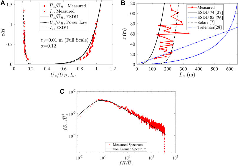
FIGURE 1. (A) Wind speed profile, turbulence intensity profile (B) integral length scale profile (in full scale dimensions) and (C) longitudinal wind velocity spectra at full-scale height, z = 76.2H.

The building model was constructed at a length scale of 1/200, equaling to the length scale of the wind field, with a height of 0.5 m, a width of 0.06 m and lengths in the range of 0.06–0.54 m. These dimensions lead to a maximum blockage ratio of 3.8%, which is lower than the maximum allowable value in ASCE 49–12 American Society of Civil Engineers(ASCE). (2012). The model was constructed with 12 removable sections such that different plan ratio configurations can be obtained by assembling different sections together. Figure 2 shows the plan view of the model (when all sections are assembled together) and the side view, together with the layout of pressure taps. There are 7 levels of pressure taps in the vertical directions in total, at heights of 0.1H, 0.3H, 0.5H, 0.65H, 0.8H, 0.9H and 0.98H, respectively. Surface pressures were measured for these models, which had plan aspect ratios ranging from 0.11 to 9, under different wind directions. Note that for configurations of D/B < 1, the same models were used with D/B ratios of their reciprocals, and measurements were taken by rotating the model, as explained in Liu et al. (2019). The Reynolds number (based on the roof height) was about 5.8 × 10⁴. The photos of the model and the wind tunnel tests can be seen in Figure 3. Other details of the experiments can be found in Liu et al. (2019).

FIGURE 2

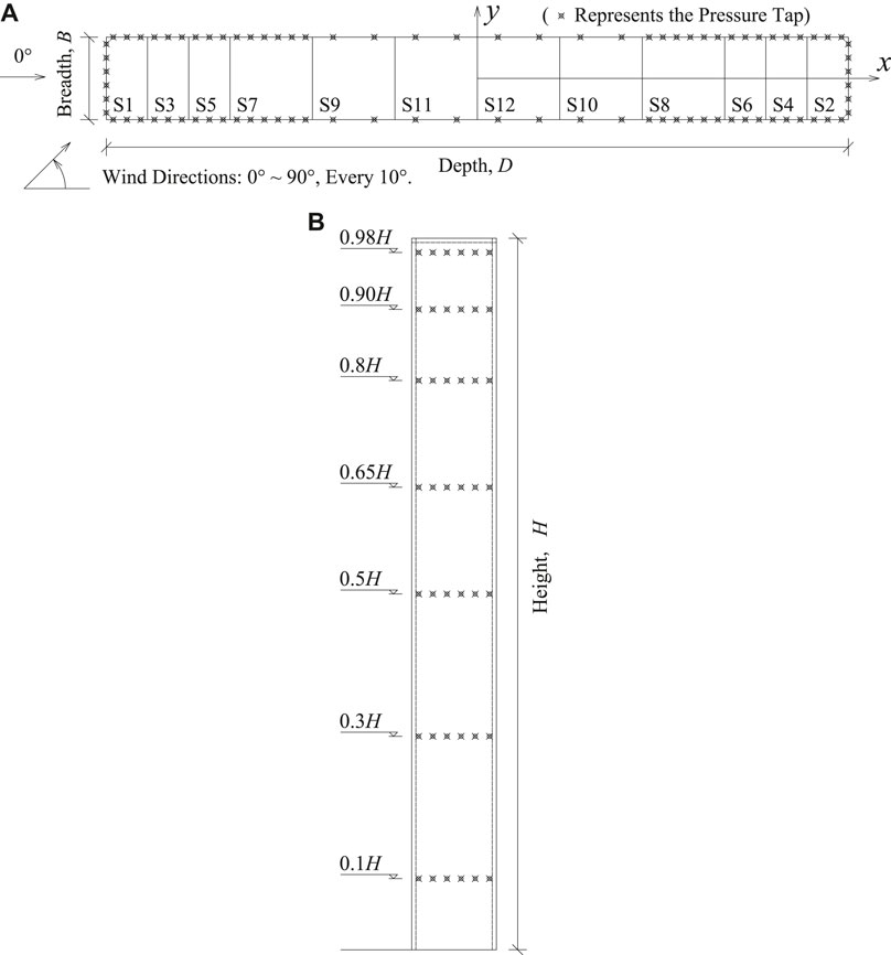
FIGURE 2. (A) Plan view and (B) side view of the model configuration for D/B = 9, including the definition of coordinate system, wind direction, and the layout of pressure taps on each section.

FIGURE 3

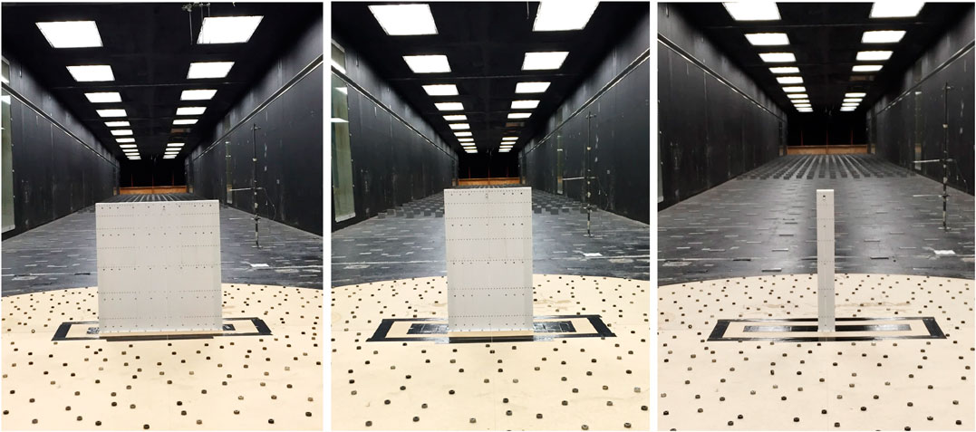
FIGURE 3. Photos of the model and wind tunnel tests.

Pressure coefficients, C_p, are referenced to the dynamic pressure at the roof height, H, following the usual convention in wind engineering. Mean and standard deviation values of C_p are denoted by ${\overline{C}}_p$, ${\sigma }_{Cp}$ (or ${C^{\prime }}_p$), respectively. Peak values, ${\widehat{C}}_p$, are estimated using the Lieblein BLUE method (Lieblein, 1976), involving dividing time series data into 10 equal segments, obtaining and rearranging 10 maxima for each and taking the mean values of Gumbel distribution as the estimated peak values. No filters of the pressure were applied such that all coefficients can be considered to be instantaneous (and, therefore, not associated with any durations beyond those associated with the tubing response).

Area-averaged pressure coefficients are obtained by integrating the pressures on each wall simultaneously, using the tributary area for each tap. Herein, we use the same symbols as for the point pressure coefficients since no point pressure coefficients are presented. In this paper, data for the two orthogonal wind directions are examined in detail. Therefore, the drag, C_d, coefficient is defined as the simultaneous difference of the area-averaged windward and leeward wall pressure coefficients. Peak value statistics of the area-averaged wall and drag coefficients are obtained in the same way as described above.

According to the definition of gust effect factor for rigid buildings in Eq. 3, the wind tunnel measured values of gust effect factor can be obtain from:

$G=\frac{{\widehat{C}}_p}{{\overline{C}}_p}\cdot \frac{0.5\rho {\overline{U}}_H^2}{0.5\rho {\widehat{U}}_H^2},(38)$

${\widehat{U}}_H=G_{ue}\cdot {\overline{U}}_H=\left(1+g_{ue}{I}_{uH}\right)\cdot {\overline{U}}_H,(39)$

where ${\widehat{U}}_H$ is the peak wind speed at roof height H, G_ue and g_ue are the empirical gust and peak velocity factors, respectively. According to Engineering Science Data Unit (ESDU). (1985), the peak factor from mean-hourly wind speed to 3 s gust speed is 3.0, thus, a value of g_ue = 3.0 is used in this paper. This value is close to the value of 2.9 in Eq. 36, which is used in ASCE 7–16.

Figure 4 shows the measured gust effect factors, G, and comparisons with the ASCE 7 value along with the results from Solari’s model (Eq. 36). Figure 5 gives the measured mean and rms (root-mean-square of the fluctuating components) area-averaged pressure coefficients or base drag coefficients along with results from Solari’s model. In Figure 5, Solari’s rms results are calculated by multiplying the rms/mean ($=2I_u\sqrt{Q_0}$; see Eq. 17) by the measured mean coefficients.

FIGURE 4

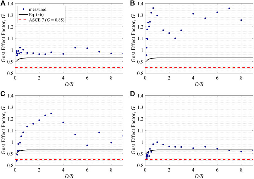
FIGURE 4. Gust effect factors for area-averaged pressure coefficients on the (A) windward wall (B) side wall (C) leeward wall, and for (D) drag coefficients under the orthogonal wind directions.

FIGURE 5

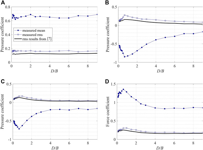
FIGURE 5. Mean and rms area-averaged pressure coefficients on the (A) windward wall (B) side wall (C) leeward wall and (D) drag coefficients under the orthogonal wind direction and comparison with results from Solari (1993a).

From Figure 4 it can be seen that Solari’s results are higher than the ASCE seven value, which is mainly due to the reduction factor of 0.925 in Eq. 37. Values from Eq. 36 tend to be smaller for lower D/B ratios, which is due to the increase of the ratio of the breadth of the building to the integral length scale, i.e., B/L_u, leading to lower values for D/B < 1. Observing the measured G values, it can be seen that, overall, most of the measured values are higher than the ASCE 7 value of 0.85, and higher than many, but not all, of the values from Eq. 36.

On the windward wall, all of the values are fairly constant with D/B ratio, with G = 1.0 ± 0.05 (Figure 4A), while the mean pressure coefficient is 0.65 ± 0.05 (Figure 5A) with a constant rms. value. Comparing to the slight decrease of G from Eq. 36 for D/B < 1, it is difficult to determine whether the measured G shows a similar trend due to the measurement uncertainties, even though the wall area is changing by a factor of 9. In contrast, for the leeward wall, there are significant and systematic changes in the measured G, with variation from 0.95 to 1.35. These values are all larger than those calculated by Eq. 36, which suggests that body generated turbulence is playing a significant role. However, the range of variation indicates complexity in the flow behavior for buildings with different D/B ratios, since the leeward wall pressures depend on the flow separating from the leeward edge of the side wall and on the wake dynamics. The systematic changes in G as a function of D/B are related to 1) the strength of the vortex shedding effects, 2) whether the separated flow from the leading edge reattaches to the side wall, and 3) turbulence generated by the leading and/or trailing edge separations, as discussed in greater detail below. It should be noted that in Figure 5B, the theoretical model results for the fluctuations are quite close to the measured values, indicating that 1) the quasi steady theory still accounts for much of the variation, and 2) the overall mismatch of G values may depend on a mismatch in the peak factors, which is analyzed in detail below. Regarding the side wall, the data are similar to those for the leeward wall, although there are subtle differences in the variation of G with D/B ratio which are related the details in the flow field.

For the drag, in contrast to the side and leeward wall cases, the measurements are significantly closer to results from Eq. 36, although the systematic variations with building geometry are greater than the theoretical model would indicate. As can be seen from Figure 4D, the model is accurate for cases where the mean flow is reattached on the side wall and the pressure is fully recovered by the leeward edge, i.e., D/B ≥ 4 (for a detailed discussion, see Liu et al., 2019). For lower D/B ratios, the theory does not capture the variation, with largest differences between the theory and the measurements of about 8%. For low D/B ratios, Eq. 36 overestimates the data, but underestimates it for 0.5 < D/B < 4. The G = 0.85 in ASCE 7 is not accurate except as D/B tends to 0. However, for D/B between 0.5 and 4, when the separation and vortex shedding effects (see below) are strongest, the theoretical model shows relatively large deviations, as it does not take these effects into account.

As discussed above, the theoretically derived gust effect factor takes into account the effects of non-contemporaneous gust actions over the building surfaces and, thus, has a value of less than 1. In contrast, the measured values indicate that either the reduction due to the non-contemporaneous effects are overestimated or offset by the amplifying effects of body-generated turbulence. Since the derivation is based explicitly on the quasi-steady assumption, only the effects of wind gustiness are taken into account while the effects of body-generated turbulence are neglected. As shown above, the body-generated turbulence appears to increase the values of G in a significant way, which is analyzed in detail in the remainder of the paper.

Aerodynamic Admittance Function

Definitions

As discussed in the previous section, the quasi-steady theory does not always hold due to the effects of non-contemporaneous gust actions over the surface and the existence of body-generated turbulence. In this section, these effects are examined in detail, by examining the aerodynamic admittance function (AAF), ${\chi }^2\left(f\right)$. The AAF is proportional to the ratio of the pressure to wind spectra and is defined via:

$S_q\left(f\right)=\frac{4{\overline{P}}^2}{{\overline{U}}^2}{\chi }^2\left(f\right)S_u\left(f\right),(40)$

where S_q is the power spectral density of the fluctuating wind pressures, and $\overline{P}$ is the mean wind pressure. From a mathematical perspective, one can view ${\chi }^2\left(f\right)$ as a correction factor in the frequency domain that connects the actual pressure fluctuations to the velocity fluctuations. It is independent of the quasi-steady assumption but helps to clarify where the quasi-steady theory holds, viz., when the value is close to 1. Values larger than one indicate the amplification of wind gusts and/or the presence of body-generated turbulence while values less than one indicate an attenuation of the wind gusts.

It can be shown that in the gust effect factor calculation, the AAF is mathematically related to spatial correlation of the wind gusts in Eq. 21. Integrating both sides of Eq. 40 over the frequency domain,

${\displaystyle {\int }_0^{\infty }{S}_q\left(f\right)}\text{d}f=\frac{4{\overline{P}}^2}{{\overline{U}}^2}{\displaystyle {\int }_0^{\infty }{\chi }^2\left(f\right)S_u\left(f\right)}\text{d}f,(41)$

${\sigma }_q^2=\frac{4{\overline{P}}^2}{{\overline{U}}^2}{\sigma }_u^2{\displaystyle {\int }_0^{\infty }\frac{S_u\left(f\right)}{{\sigma }_u^2}{\chi }^2\left(f\right)}\text{d}f,(42)$

i.e.,

${\sigma }_q=2\overline{P}{I}_u\sqrt{A_0},(43)$

$A_0={\displaystyle {\int }_0^{\infty }\frac{S_u\left(f\right)}{{\sigma }_u^2}{\chi }^2\left(f\right)}\text{d}f,(44)$

Similarly,

${\sigma }_{\dot{q}}=2\overline{P}{I}_u\frac{2\pi {\overline{U}}_z}{L_u}\sqrt{A_1},(45)$

$A_1={\displaystyle {\int }_0^{\infty }{\left[\frac{f{L}_u}{{\overline{U}}_z}\right]}^2\frac{S_u\left(f\right)}{{\sigma }_u^2}{\chi }^2\left(f\right)}\text{d}f.(46)$

Comparing Eq. 44 with Eq. 19, one can see that ${\chi }^2\left(f\right)$ and $\chi \left(f\right)$ are synonymous (noting that the moving average filter is not included in Eq. 44). Thus, we use these terms interchangeably, although the physical meaning of the two are somewhat different. To obtain the gust effect factor using the AAF and without the moving average, A₀ replaces Q₀ in Eqs 17, 18, while A₁ replaces Q₁ in Eq. 18. To obtain the gust effect factor using the AAF and with the moving average filter, X (f, τ) is added to Eqs 44, 46.

A commonly used form of the AAF is Vickery’s model (Vickery, 1965):

$\chi \left(f\right)=\frac{1}{1+{\left[\frac{2f\sqrt{A}}{\overline{U}}\right]}^{4/3}},(47)$

where A is the frontal area, which is BH for the current buildings. This model was obtained from drag force data for two-dimensional bluff bodies in contrast to Eq. 21, which was derived based on the spatial correlation of wind speeds and does not consider the effects of body-generated turbulence. Figure 6 provides the AAFs for the area-averaged fluctuating pressures on the side wall, together with Eq. 47 and Eq. 21, the latter of which is used in the ASCE 7 implementation. It is also noted that, while these models may not be expected to hold for single surfaces such as the side walls in Figure 6, the provisions of Chapter 27 in ASCE 7–16 use gust effect factors for single walls to develop the overall loads, so it is of practical importance to understand how well this works.

FIGURE 6

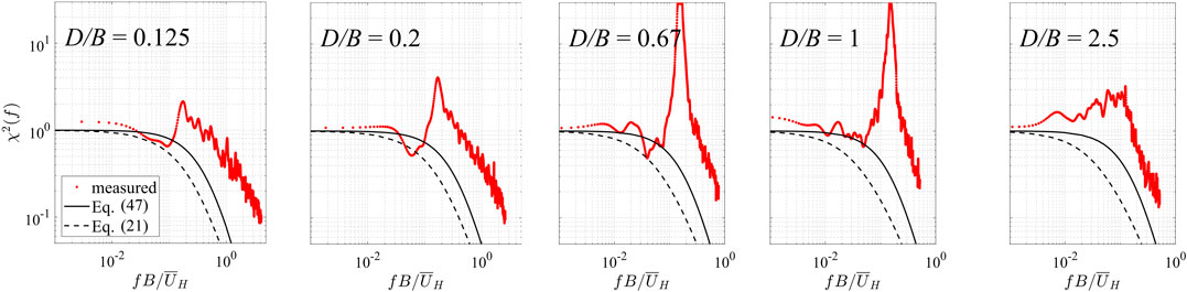
FIGURE 6. Aerodynamic admittance functions for area-averaged fluctuating pressure coefficients on the side wall. Legends: measured, Eq. 47, Eq. 21.

Experimental Results

For the AAF on side walls, as can be seen in Figure 6 there is an obvious peak indicating vortex shedding for D/B < 2.5. The peak reaches its highest energy level for D/B between 0.5 and 1. For lower D/B values, the peak decreases, indicating the relative less separation and vortex shedding effects on the building side walls. For D/B > 1, the after-body, (i.e. the distance from the separation point) is larger and the flow either partially or fully reattaches. In this range, the vortex shedding has relatively more variability as indicated by the broad-band peak. For D/B ≥ 2.5, the mean flow is reattached on the side wall (see Liu et al. (2019), who determined this based on the method given by Akon and Kopp (2016) for elevations between 0.2H–0.8H), and the vortex shedding peak is eliminated. The Strouhal number, St, using the peaks in determined from the side-wall spectra, are shown in Figure 7. Figure 7 also includes data from Liang et al. (2002) and Lander et al. (2016). It can be seen that the Liang et al. (2002) values are smaller than those from current data. However, closer values are obtained for the square prism data (D/B = 1) of Lander et al. (2016).

FIGURE 7

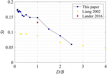
FIGURE 7. Strouhal number as a function of D/B ratio.

FIGURE 8

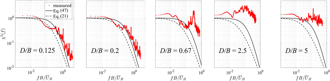
FIGURE 8. Aerodynamic admittance functions for area-averaged fluctuating pressure coefficients on the leeward wall.

As can be seen in Figure 8, for the leeward walls, the vortex shedding peaks remain, although they are significantly reduced in magnitude and are at twice the Strouhal number since the leeward side is influenced by vortices from both sides of the wake. The vortex shedding peak is clearly evident over the range 0.5 ≤ D/B ≤ 2.5. For D/B < 0.5, the vortex shedding peak is not evident and the AAF closely follows Vickery’s model (Eq. 47) while being slightly larger than Solari’s formulation (Eq. 21) at the higher frequencies. For D/B > 2.5, the flow on the side wall is reattached with full pressure recovery by D/B > 4. In this case there is significant energy at higher frequencies, which must be due to the separation of the turbulent boundary layers at the leeward edge. The AAF for drag are depicted in Figure 9. There is little evidence of the vortex shedding on these results, although there is a tendency to significant energy at the higher frequencies, which may be affected by the vortex shedding in the range 0.5 ≤ D/B ≤ 2.5 and the separated turbulent flow for D/B > 2.5. Overall, both Vickery’s and Solari’s model slightly underestimate the data at the higher frequencies.

FIGURE 9

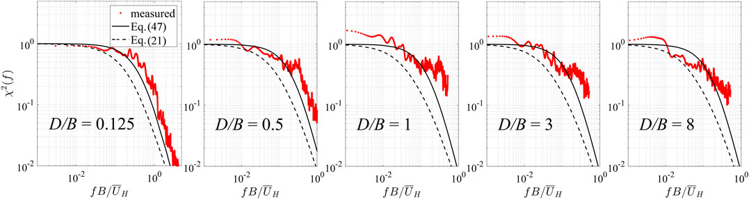
FIGURE 9. Aerodynamic admittance functions for drag coefficients.

As can be seen from analysis above, the AAF reflects some important characteristics of the flow and the fluctuating pressures in the frequency domain, which directly influences the value of G in Eq. 17 through $\sqrt{Q_0}$ in Eq. 19 or $\sqrt{A_0}$ in Eq. 44. However, because of the square-root dependence, small errors in the AAF will not play a significant role in creating errors in G. The empirical model of Vickery (Eq. 47) is slightly more accurate than that based solely on the analysis of the wind field, as developed by Solari (Eq. 21). Thus, the AAF for the drag coefficient would appear to be sufficiently accurate, with larger errors for the individual walls, particularly the side walls where the vortex shedding is strongest. Therefore, the differences between the measured and theoretical gust effect factors depicted in Figure 4D in the range 0.5 ≤ D/B ≤ 4 must be due to other factors in the formulation, e.g., the peak factor, g_q, and the moving average filter, X (f, τ). These are examined in the next two sections, respectively.

Peak factors and moving-average duration of the response

Peak Factors

Figure 10 depicts the measured peak factors, g_q, with comparisons to the theoretical values (Eq. 18). As can be seen from Figure 10, most of the measured peak factors are larger than 3.0. For side wall pressures, as Figure 6 shows, the case which shows strongest separation and vortex shedding effects occurs at D/B = 0.67, with a peak factor of about 4.5. However, for D/B of 0.25–0.5, the peak factor reaches about 5.0. Saathoff and Melbourne (1989) argues that the generation of large negative peak pressures in separated flows is related to unstable intermittent roll-up of the separated shear layers; thus, the increase in peak factors may be caused by relatively more synchronous roll-up of the shear layers over the entire, but smaller, side surface. For D/B < 0.25, the peak factor decreases, which can be mainly attributed to the weaker turbulence effects as the separated shear layer develops. As D/B increases above 1, the flow is partially reattached on the side wall, leading to lower correlations over the surface such that the peak factor decreases. For D/B ≈ 2.5, the mean flow is reattached on the side wall and the peak factor is about 3.5 for lager D/B values.

FIGURE 10

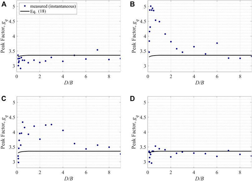
FIGURE 10. Measured and predicted peak response factors, g_q, for area-averaged pressure coefficients on the (A) windward wall, (B) side wall, (C) leeward wall and for (D) drag coefficients under the orthogonal wind direction.

The data are similar for leeward wall pressures where, for D/B ratios between 0.25 and 4, the peak factor is larger than 4.0. For D/B < 0.25, due to relatively weaker turbulence effects, the peak factor is reduced. The peak factor is also reduced for D/B > 4. Overall, for pressures on the side and leeward walls, most of the peak factors are significantly larger than 3.0. However, for windward walls the peak factors are between 3.0 and 3.5, which is also true for the drag.

Comparing the measured peak factors to the theoretical values, as can be seen in Figure 10, estimated values of g_q using Eq. 18, which are all between 3.3 and 3.4, show significant differences from measured values for the side and leeward walls. For D/B smaller than 2.5 on the side wall and for D/B between 0.25 and four on the leeward wall, the measured values are significantly larger than the theoretical values. This is due to Eq. 18 being based on the assumption that the fluctuating pressures constitute a Gaussian process, based on the quasi-steady assumption. However, as can be seen from Figure 11, where some typical probability distributions are given, this assumption does not always hold. For pressures on the side wall, the probability distribution is significantly left-skewed from the Gaussian distribution; while for base drag, the probability is slightly right-skewed from the Gaussian distribution. There have been many studies regarding estimating peak factors for non-Gaussian processes, such as Kareem and Zhao (1994), Kwon and Kareem (2011) and Huang et al. (2013). Many of the studies use skewness and kurtosis of the non-Gaussian process to predict the peak factor. Here, the methods for estimating peak factors are not focused. In the following section, measured g_q values are directly used to calculate G_Q and G values, to focus on the effects of the moving average filter, X (f, τ).

FIGURE 11

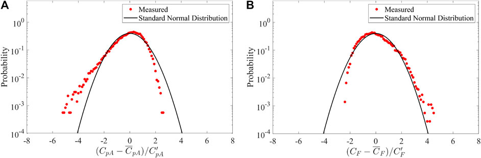
FIGURE 11. Probability distributions for D/B = 1 for (A) area-averaged pressure coefficients on the side wall and (B) drag coefficients.

Moving-Average Duration

In this section, the effects of the moving average filter are examined. Figure 12 shows the measured G values, together with the comparison to the theoretical values. Note that the measured 3 s moving average response is obtained by using Eq. 23 with the measured g_q and Q₀ values. The difference in the measured instantaneous and 3 s duration values represents the load effects of the small-scale turbulence in the wind as well as the body-generated turbulence. The difference between the measured 3 s duration and the theoretical values represent the effects of the other factors in the model including the peak factors and force or pressure spectrum. Several observations can be made, first, for the windward wall, the match between all of the curves is good with generally small cumulative difference in all of the curves. Clearly, the effect of duration is minimal for windward walls where there are limited small-scale turbulence effects after spatial averaging. Second, in contrast, there are clear duration effects on the side wall for D/B between about 0.5 and 2.5, i.e., for plan dimensions where the separated shear layer is playing a dominant role, which is most significant for D/B between about 0.5 and 1. Third, for the leeward wall, the body-generated turbulence also has a significant effect over D/B between about one and 4. Finally, the drag force does exhibit some dependence on the body-generated turbulence, the effects are only slightly larger than those on the windward wall. In fact, the bulk of the difference between the theoretical gust factor and the measured values for the drag are due to body-generated turbulence for 0.5 < D/B < 4 (caused by the leeward walls contribution), while for D/B < 0.5, it is due to the peak factor.

FIGURE 12

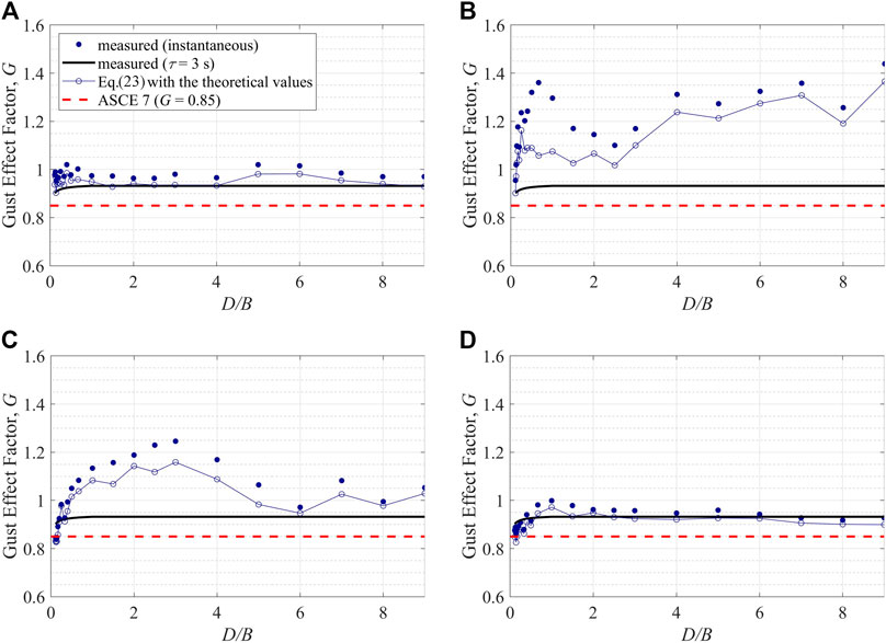
FIGURE 12. Measured and predicted gust effect factor, G, for area-averaged pressure coefficients on the (A) windward wall (B) side wall (C) leeward wall and for (D) base drag coefficients under the orthogonal wind direction.

Conclusion

The objective of the paper is to systematically investigate the gust effect factor for rigid high-rise buildings based on an experimental approach. From the analysis of the data, the following conclusion can be made:

(1) The aerodynamic admittance function (AAF) reflects important characteristics of the fluctuating pressures in the frequency domain and has direct influence on the value of the gust effect factor. For pressures on the windward wall and base drag, AAF decreases with frequency for high frequencies, meaning that the effects of non-contemporaneous gust actions are playing a leading role. This leads to gust effect factors that usually have values less than (or close to) unity. For the side and leeward wall pressures, the combined effects of separation, vortex shedding and reattachment lead to large peaks in AAF causing the gust effect factor to have values larger than unity.

(2) The statistical distributions of the fluctuations affect the peak factors. Non-Gaussian behavior is observed, which significantly affects the side and leeward wall peak factor for 0.5 < D/B < 4. For D/B < 0.5, the side wall area is small and it appears that the vortices in the separated shear layer may not be sufficiently formed to affect the fluctuating pressures substantially. For D/B > 4, the separated shear layers reattach on the side walls and there is sufficient distance for full pressure recovery prior to the leeward edge. Evidently, this also reduces the effects on the peak factors, indicating limited effects of body-generated turbulence.

(3) The effects of moving average time are similar to those of peak factors. For building geometries and surfaces with significant body-generated turbulence, the moving average duration has a significant effect. Thus, for side and leeward walls in the range 0.5 < D/B < 4, there are significant effects. For windward walls and overall drag, the effect of duration is minimal.

(4) Overall, the results in the ASCE 7–16 gust effect factor for rigid buildings are underestimated for many building configurations. The main reasons are: 1) the term in the formulation which characterizes the non-contemporaneous gust actions, i.e. the theoretical AAF, underestimates actual conditions, due to the neglect of the body-generated turbulence effects; 2) the underestimation of the peak factor, due to the limited applicability of the estimating method, which is only suitable for Gaussian processes, while actual conditions usually show significant non-Gaussian characteristics; and 3) the use of the 3 s moving average filter. These lead to significant underestimates for side and leeward walls, while the windward wall is low by less than 5% on average. Overall, the gust factor for the drag force is well-estimated theoretically, except for 0.5 ≤ D/B ≤ 1, where it is low by about 5% due to the effects of body-generated turbulence on the leeward wall. Thus, one can conclude that the gust factor model for rigid buildings works well for the drag but much less well for individual wall-averaged pressure coefficients.

Data Availability Statement

The raw data supporting the conclusion of this article will be made available by the authors, without undue reservation.

Author Contributions

YL developed the hypothesis for the paper, conducted the experiments, analyzed the data, and wrote the first draft of the paper. GK and SC both guided the overall work, the experimental design, and data analyses, and edited the manuscript.

Funding

NSERC Canada funded the experimental portion of the study, under a Discovery Grant held by GK. YL received a scholarship from China Scholarship Council.

Conflict of Interest

The authors declare that the research was conducted in the absence of any commercial or financial relationships that could be construed as a potential conflict of interest.

Acknowledgments

YL gratefully acknowledges financial support from the China Scholarship Council. GK acknowledges financial support for the wind tunnel experiments from the NSERC Discovery Grants program.

References

Akon, A. F., and Kopp, G. A. (2016). Mean pressure distributions and reattachment lengths for roof-separation bubbles on low-rise buildings. J. Wind Eng. Ind. Aerod. 155, 115–125. doi:10.1016/j.jweia.2016.05.008

CrossRef Full Text | Google Scholar

American Society of Civil Engineers (ASCE) (1993). ASCE standard, minimum design loads for buildings and other structures. Reston, VA, United States: ASCE, 7–93.

Google Scholar

American Society of Civil Engineers (ASCE) (2016). ASCE standard, minimum design loads for buildings and other structures. Reston, VA, United States: ASCE, 7–16.

Google Scholar

American Society of Civil Engineers (ASCE) (2012). ASCE Standard, Wind tunnel testing for buildings and other structures. Reston, VA, United States: ASCE, 49–12.

Google Scholar

Davenport, A. G. (1963). The buffeting of structures by gusts. Proceedings of International Conference on Wind Effects on Buildings and Structures, Teddington, Middlesex, United Kingdom, 1963, 358–391.

Google Scholar

Davenport, A. G. (1964). Note on the distribution of the largest value of a random function with application to gust loading. Proc. Inst. Civ. Eng. 28(2), 187–196. doi:10.1680/iicep.1964.10112

CrossRef Full Text | Google Scholar

Davenport, A. G. (1967). Gust loading factors. J. Struct. Div. 93 (3), 11–34. doi:10.1061/jsdeag.0001692

CrossRef Full Text | Google Scholar

Engineering Science Data Unit (ESDU) (1974). Characteristics of atmosphere turbulence near the ground, Part 2: single point data for strong winds (neutral atmosphere) ESDU 74031, London, United Kingdom: ESDU.

Google Scholar

Engineering Science Data Unit (ESDU) (1982). Strong winds in the atmosphere boundary layer, Part 1: mean-hourly wind speeds ESDU 82026, London, United Kingdom: ESDU.

Google Scholar

Engineering Science Data Unit (ESDU) (1985). Characteristics of atmosphere turbulence near the ground, Part 2: single point data for strong winds (neutral atmosphere) ESDU 85020, London, United Kingdom: ESDU.

Google Scholar

Greenway, M. E. (1979). An analytical approach to wind velocity gust factors. J. Wind Eng. Ind. Aerod. 5 (1-2), 61–91. doi:10.1016/0167-6105(79)90025-4

CrossRef Full Text | Google Scholar

Holmes, J. D. (2015). Wind loading of structures. Boca Raton, FL, United States: CRC Press.

Google Scholar

Huang, M. F., Lou, W., Chan, C. M., Lin, N., and Pan, X. (2013). Peak distributions and peak factors of wind-induced pressure processes on tall buildings. J. Eng. Mech. 139 (12), 1744–1756. doi:10.1061/(asce)em.1943-7889.0000616

CrossRef Full Text | Google Scholar

Kareem, A., and Zhao, J. (1994). Analysis of non-Gaussian surge response of tension leg platforms under wind loads. J. Offshore Mech. Arctic Eng. 116 (3), 137–144. doi:10.1115/1.2920142

CrossRef Full Text | Google Scholar

Kareem, A., and Zhou, Y. (2003). Gust loading factor—past, present and future. J. Wind Eng. Ind. Aerod. 91 (12-15), 1301–1328. doi:10.1016/j.jweia.2003.09.003

CrossRef Full Text | Google Scholar

Kijewski, T., and Kareem, A. (1998). Dynamic wind effects : a comparative study of provisions in codes and standards with wind tunnel data. Wind Struct. 1 (1), 77–109. doi:10.12989/was.1998.1.1.077

CrossRef Full Text | Google Scholar

Kwon, D. K., and Kareem, A. (2011). Peak factors for non-Gaussian load effects revisited. J. Struct. Eng. 137 (12), 1611–1619. doi:10.1061/(asce)st.1943-541x.0000412

CrossRef Full Text | Google Scholar

Kwon, D. K., and Kareem, A. (2014). Revisiting gust averaging time and gust effect factor in ASCE 7. J. Struct. Eng. 140 (11), 06014004. doi:10.1061/(asce)st.1943-541x.0001102

CrossRef Full Text | Google Scholar

Lander, D. C., Letchford, C. W., Amitay, M., and Kopp, G. A. (2016). Influence of the bluff body shear layers on the wake of a square prism in a turbulent flow. Physical Review Fluids. 1 (4), 044406. doi:10.1103/physrevfluids.1.044406

CrossRef Full Text | Google Scholar

Liang, S., Liu, S., Li, Q. S., Zhang, L., and Gu, M. (2002). Mathematical model of acrosswind dynamic loads on rectangular tall buildings. J. Wind Eng. Ind. Aerod. 90 (12-15), 1757–1770. doi:10.1016/s0167-6105(02)00285-4

CrossRef Full Text | Google Scholar

Lieblein, J. (1976). Efficient methods of extreme-value methodology, Paris, France: Nuclear Energy Agency.

Google Scholar

Liu, Y., Kopp, G. A., and Chen, S.-f. (2019). Effects of plan dimensions on gust wind loads for high-rise buildings. J. Wind Eng. Ind. Aerod. 194, 103980. doi:10.1016/j.jweia.2019.103980

CrossRef Full Text | Google Scholar

Piccardo, G., and Solari, G. (2002). 3-D gust effect factor for slender vertical structures. Probabilist. Eng. Mech. 17 (2), 143–155. doi:10.1016/s0266-8920(01)00034-0

CrossRef Full Text | Google Scholar

Saathoff, P. J., and Melbourne, W. H. (1989). The generation of peak pressures in separated/reattaching flows. J. Wind Eng. Ind. Aerod. 32 (1-2), 121–134. doi:10.1016/0167-6105(89)90023-8

CrossRef Full Text | Google Scholar

Simiu, E. (1977). Equivalent static wind load for tall building design. Proceedings of the 4th international conference on wind engineering. London, United Koingdom: Cambridge University.

Google Scholar

Solari, G. (1988). Equivalent wind spectrum technique: theory and applications. J. Struct. Eng. 114 (6), 1303–1323. doi:10.1061/(asce)0733-9445(1988)114:6(1303)

CrossRef Full Text | Google Scholar

Solari, G. (1993a). Gust buffeting. I: peak wind velocity and equivalent pressure. J. Struct. Eng. 119 (2), 365–382. doi:10.1061/(asce)0733-9445(1993)119:2(365)

CrossRef Full Text | Google Scholar

Solari, G. (1993b). Gust buffeting. II: dynamic alongwind response. J. Struct. Eng. 119 (2), 383–398. doi:10.1061/(asce)0733-9445(1993)119:2(383)

CrossRef Full Text | Google Scholar

Solari, G., and Kareem, A. (1998). On the formulation of ASCE7-95 gust effect factor. J. Wind Eng. Ind. Aerod. 77-78, 673–684. doi:10.1016/s0167-6105(98)00182-2

CrossRef Full Text | Google Scholar

Stathopoulos, T. (1983). Fluctuating wind pressures on low building roofs. J. Struct. Eng. 109 (1), 266–271. doi:10.1061/(asce)0733-9445(1983)109:1(266)

CrossRef Full Text | Google Scholar

Tieleman, H. W. (2003). Roughness estimation for wind-load simulation experiments. J. Wind Eng. Ind. Aerod. 91, 1163–1173. doi:10.1016/s0167-6105(03)00058-8

CrossRef Full Text | Google Scholar

Vickery, B. J. (1965). On the flow behind a coarse grid and its use a model of atmospheric turbulence in studies related to wind loads on buildings. NPL Aero Report. 1143.

Google Scholar

Vickery, B. J. (1970). On the reliability of gust loading factors, Washington, DC, United States.: Proceedings of Technical Meeting Concerning Wind Loads on Buildings and Structures, 93–104.

Google Scholar

Wu, C. H., and Kopp, G. A. (2016). Estimation of wind-induced pressures on a low-rise building using quasi-steady theory. Frontiers in built environment. 2, 5. doi:10.3389/fbuil.2016.00005

CrossRef Full Text | Google Scholar

Zhou, Y., Kareem, A., and Gu, M. (1999). Gust loading factors for design applications. Copenhagen, Denmark: Proceedings of the 10th International Conference on Wind Engineering, 169–176.

Google Scholar

Zhou, Y., and Kareem, A. (2001). Gust loading factor: New model. J. Struct. Eng. 127 (2), 168–175. doi:10.1061/(asce)0733-9445(2001)127:2(168)

CrossRef Full Text | Google Scholar

Zhou, Y., Kijewski, T., and Kareem, A. (2002). Along-wind load effects on tall buildings: comparative study of major international codes and standards. J. Struct. Eng. 128 (6), 788–796. doi:10.1061/(asce)0733-9445(2002)128:6(788)

CrossRef Full Text | Google Scholar