Motion Design with Efficient Actuator Placement for Adaptive Structures that Perform Large Deformations

Introduction

Sustainability and energy efficiency have become important design requirements for engineering structures. The ability to adapt to changing loading conditions enables adaptive structures to achieve material and energy savings. Through sensing and actuation, adaptive structures are able to counteract deflections and to homogenize the stress under varying loading conditions as shown in Sobek and Teuffel (2001) and Senatore et al. (2018). In so doing significant mass, embodied energy and carbon can be saved compared to conventional passive structures. Since these studies were primarily concerned with adaptive load-bearing structures, adaptation was limited to relatively small shape changes.

Adaptive structures can also adapt to varying usage requirements during service, for example, deployable structures in the form of retractable roofs, folding bridges and adaptive façades (e.g., Knippers and Schlaich 2000; Knippers et al., 2013). In these cases, the structure adapts through a series of geometry configurations that might differ significantly from each other. Transitioning from one geometry configuration to another is typically carried out through articulations such as joints and hinges, or in the case of compliant structures, by a targeted stiffness reduction in the direction of the desired deformation (Kota et al., 2001). Compliant structures (also called morphing structures) are able to deform in required shapes through strategic distribution of stiffness as shown in Hasse and Campanile (2009), and Masching and Bletzinger (2016). Several studies also exist on truss (Inoue 2008; Sofla et al., 2009; Reksowardojo et al., 2019) and tensegrity structures (Wijdeven and Jager 2005; Masic and Skelton 2005) that are able to perform large shape changes.

A critical aspect in structural adaptation is to consider the transition between shapes (i.e., geometry configurations) because changing shape causes stresses and requires energy. The shape change can be realized through different actuation types. Discrete (e.g., linear) and continuous (e.g., piezoelectric, shape-memory alloy) actuators have been employed for shape control (Irschik 2002, Mohd Jani et al., 2014, Senatore et al., 2018). The way the actuators are controlled is important to achieve satisfactory shape-control efficiency. Other approaches combine optimal control with mechanics (Preumont 2011; Ibrahimbegovic et al., 2004) as well as stochastic optimization with path-planning and machine learning (Veuve et al., 2017; Sychterz and Smith 2018).

Optimal actuator placement is a key to shape control efficiency. This is a challenging task i.e., an active field of research. Generally, the better the choice of the actuator locations, the lower the energy for adaptation. Actuator placement has been carried out through numerical optimization formulations in Gupta et al. (2010) with a focus on the use of piezoelectric actuation. In Kwan and Pellegrino (1993), a simplex optimization approach was applied for actuator placement in pre-stressed deployable structures. Actuator placement formulations for discrete truss structures have been given by many. A genetic optimization algorithm was implemented for efficient structural vibration control in Abdullah et al. (2001). A greedy and inverse greedy algorithm was implemented by Wagner et al. (2018) for optimal compensation of external disturbances. In Teuffel (2004), optimal placement was implemented based on a heuristic measure of actuator efficacy for force and shape control. Senatore et al. (2019) and Wang and Senatore (2020) formulated new methods to design minimum energy adaptive structures. Embodied energy in the material and operational energy for control are minimized through combined optimization of structural sizing and actuator placement. Results have shown that minimum energy adaptive structures perform significantly better than conventional passive structures with regard to input material as well as energy and carbon requirements thus reducing adverse environmental impacts. These studies focused on load-bearing structures and thus were based on small strain and small displacement assumptions. Large deformations have been accounted for in Masching and Bletzinger (2016), where actuator locations were optimized based on a measure of control efficiency which is included in the shape optimization of shells. A multi-objective optimization formulation was given in Reksowardojo et al. (2020) to design truss structures that react to loading through shape adaptation accounting for large deformations. The structure is designed to “morph” into shapes that are optimal to take external loads. These target shapes are obtained through shape optimization. The actuator placement is then optimized so that the structure can be controlled into the target shapes. The inverse problem to obtain actuator commands that control the structure into the target shapes is solved through a Newton-Raphson scheme based on a geometrically nonlinear force method. It was shown that optimal shape adaptation enables significant stress homogenization which produces minimum mass structural solutions.

In this publication, heuristic algorithms for actuator placement are combined with an existing method for motion design presented in Sachse and Bischoff (2020) and further extended in Sachse et al. (2021). This method produces optimal deformation paths between two prescribed geometric configurations that might differ significantly from each other to meet varying demands during service. The method of motion design takes large deformations into account. Motion might involve element deformations, deployment through finite mechanisms and a combination of both. The integral of the strain energy over the deformation path is employed as the objective function, which is to be minimized. This objective can be interpreted as the “cost of deformation,” which is similar to the “cost of transport” employed in robotics (e.g., Seok et al., 2013). The “cost of deformation” gives an indication of the energy required to control the structure between two prescribed shapes. In Sachse and Bischoff (2020) this method was investigated for structures that move through finite mechanisms, incorporating instability behavior and inextensible deformations of shells. The optimal motion trajectory is first obtained. Then, actuation forces to realize such motion are back-calculated from equilibrium conditions. As a result, actuation forces may be required for all degrees of freedom, which is a limitation for most practical structures since the actuation system would be too complex. This limitation has been surpassed by adding suitable constraints to the motion design formulation so that resulting deformation paths can be realized through a specific number of external or internal actuators. The constrained motion design formulation is given in Sachse et al. (2021) and is summarized in Motion Design of Structures With Constraints of this paper for completeness. A method for optimal placement of external actuation forces to control the structure into required deformation paths is given in Motion Through External Actuation. In Motion Through Internal Actuation, a similar method is implemented for optimal placement of internal actuators.

In none of the methods presented in this work constraints on material strength and stability (local and global) are considered to ensure that structural integrity is preserved throughout the motion. Applying the formulation presented in this paper to load-bearing structures is not feasible and requires appropriate extensions.

Motion Design of Structures With Constraints

Basic Method of Motion Design

As described in Sachse and Bischoff (2020), the motion design method enables to identify an optimal deformation path between an initial undeformed geometry and a prescribed deformed configuration. Figure 1A shows an illustration of this method. The initial geometry (black), as well as the deformed final geometry (blue) of a two-bar truss, is given and the optimal trajectory of point P (red) is searched for. It is also possible to prescribe only parts of the end-configuration, e.g., only a vertical displacement. The method is developed for quasi-static problems that do not include dynamic effects and for geometrically nonlinear problems accounting for large deformations. The functional J, i.e., the objective function that is to be minimized, is the integral of the strain energy Π_int over the deformation path s

$\mathit{J}\mathrm{=}{\displaystyle \underset{\mathit{s}}{\int }{\displaystyle {\Pi }_{\mathrm{int}}\mathit{ds}\to \min }}.(1)$

Using the Green-Lagrange strain tensor E, second Piola-Kirchhoff stress S and the linear, elastic and isotropic St. Venant-Kirchhoff material law for large deformations with the elasticity tensor C, the strain energy is therein defined as

${\Pi }_{\mathit{int}}\mathrm{=}{\displaystyle {\int }_{\mathit{\Omega }}\frac{\mathrm{1}}{\mathrm{2}}{\mathbf{E}}^{\mathbf{T}}\mathbf{S}\mathit{ }\mathrm{d}\mathit{\Omega }}\mathrm{=}{\displaystyle {\int }_{\mathit{\Omega }}\frac{\mathrm{1}}{\mathrm{2}}{\mathbf{E}}^{\mathbf{T}}\mathbf{CE }\mathit{ }\mathrm{d}\mathit{\Omega }}(2)$

J is a measure for the “cost of deformation.” To solve this problem using variational calculus, two discretizations are introduced. The first is the well-known spatial discretization of the structure, i.e., the discretization with a number of finite elements n_ele. This allows the unknown displacement field to be approximated using n_dof discrete displacement degrees of freedom (i.e., nodal displacements), which are combined in the vector D(s). By using bar elements as in the illustrative example in Figure 1, the structure is already discretized in space by its nature. However, the method can also be used with other finite element formulations in two or three dimensions as well as with other spatial discretizations such as Lagrange and Non-Uniform Rational B-Spline (NURBS-) shape functions. The nodal displacements, i.e., the displacement field, are the variables that are searched for.

FIGURE 1

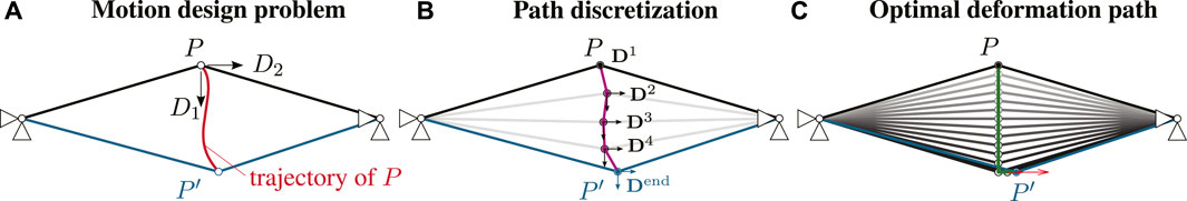
FIGURE 1. Motion design of a two-bar truss. (A) Motion design Problem, (B) Path discretization, and (C) Optimal deformation path.

The nodal displacements are functions of the deformation path, since the displacement field changes throughout the motion. Due to this dependence on the motions, a second discretization of the deformation path is introduced, as illustrated in Figure 1B. This can be compared to space-time finite elements but differs in the fact that the deformation path depends on the displacement field while time is an autonomous value. The deformation path is discretized with ${\overline{n}}_{\text{ele}}$ path elements between the initial configuration and the prescribed end-configuration. For clarity, n_ele denotes the number of structural elements while ${\overline{n}}_{\text{ele}}$ the number of motion-path elements (for brevity path elements). This way the integral in the objective function can be split into a sum over all motion-path elements:

$J=\underset{s}{{\displaystyle \int }}{\text{Π}}_{\text{int}} \text{d}s\approx {\displaystyle \sum }_{e=1}^{{\overline{n}}_{\text{ele}}}\underset{s_e}{{\displaystyle \int }}{\text{Π}}_{\text{int}} \text{d}{s}_e.(3)$

Considering a discretization with ${\overline{n}}_{\text{ele}}$ path elements and associated ${\overline{n}}_{\text{node}}$ path nodes, the total number of degrees of freedom increases to

${\overline{n}}_{\text{dof}}={\overline{n}}_{\text{node}}\cdot n_{\text{dof}}.(4)$

The motion-path nodes are intermediate geometric configurations that are encountered throughout the motion. The relationship between the number of motion-path nodes ${\overline{n}}_{\text{node}}$ and elements ${\overline{n}}_{\text{ele}}$ depends on the employed shape functions. The shape functions in this discretization interpolate the initial, intermediate and end-configuration. Generally, all types of shape functions, which interpolate the different geometric configurations, can be used for the deformation-path discretization, e.g., Lagrange polynomials as well as B-spline functions. Depending on the problem, a suitable discretization method should be chosen. The vector of total displacement degrees of freedom $\overline{\mathrm{D}}$ is extended since it contains degrees of freedom of all geometric configurations throughout the motion and therefore consists of ${\overline{n}}_{\text{node}}$ vectors

$\overline{\mathrm{D}}=\left[\begin{array}{c}{\mathbf{D}}^1\\ {\mathbf{D}}^2\\ \dots \\ {\mathbf{D}}^{{\overline{n}}_{\text{node}}}={\mathbf{D}}^{\text{end}}\end{array}\right](5)$

where ${\mathbf{D}}^1=\mathbf{0}$ and D^end refer to the initial (undeformed) and end-configuration (prescribed target shape), respectively. The constraint of reaching the target shape is included by prescribing the displacement values within the vector D^end. In the example of Figure 1B a motion discretization of four linear elements is employed, which leads to

$\overline{\mathbf{D}}={\left[D_1^1 D_2^1 D_1^2 D_2^2 D_1^3 D_2^3 D_1^4 D_2^4 D_1^{\text{end}} D_2^{\text{end}}\right]}^T.(6)$

The superscripts indicate the geometric configuration throughout the motion while the subscripts indicate the nodal displacement degrees of freedom. Building the variation leads to a nonlinear system of equations that can be solved iteratively through linearization using the Newton-Raphson solution scheme. This way, the deformation path is obtained for all configurations at once rather than incrementally, as is the case in nonlinear structural analysis. As the end-configuration is prescribed, the value of the strain energy at the end of the deformation path cannot be changed. However, the intermediate configurations are varied such that the integral of the strain energy is minimized. The solution of the motion of the two-bar-truss example using 14 linear path elements is illustrated in Figure 1C. A vertical snap-through with a successive motion to the right side causes less integrated strain energy than a linear interpolation between the initial and end-configuration. The solution is not unique because various discretizations may approximate the same curve. As a result, the problem is not well-posed and it has to be regularized by either enforcing equal size of the path elements or by controlling the increment of a chosen degree of freedom throughout the motion (Sachse and Bischoff, 2020).

The resulting motion is realized by applying forces to the structure. Equilibrium conditions have not been considered because equilibrium can be enforced for any resulting optimal deformation path since it is assumed that arbitrary forces can be applied at any degree of freedom. The internal forces are calculated throughout the entire deformation process using the displacement values. For equilibrium, the internal forces are then set as the external actuation forces required to realize the deformation path. In other words, external forces are determined that are in equilibrium with all deformed configurations. In practice, this means that external actuation forces (i.e., point forces at nodes), might need to be applied to all degrees of freedom. This is usually not of concern when the motion is realized through finite mechanisms (e.g., deployable structures). In such cases, considering frictionless finite mechanisms, absence of gravity and no external loading, the external actuation forces are zero. However, if the motion is not realized through finite mechanisms and for structures that are made of many elements, this assumption would lead to prohibitively complex actuation systems. In such cases, it is possible to formulate suitable constraints so that the motion is controlled through a prescribed number of internal or external actuators. This approach has been presented in Sachse et al. (2021) and it is summarized in the following.

Constrained Motion Design With a Prescribed Number of Actuators

Consider the configuration illustrated in Figure 2. In unconstrained motion design, all free degrees of freedom are controlled by forces F₁, F₂, and F₃ as in Figure 2A. In constrained motion design, the deformation path is controlled through a subset of forces, F₁ and F₂ as shown in Figure 2B. Therefore, F₃ is set to zero throughout the motion. This is a constraint on the solution and can be introduced in the functional by different constraint-enforcement techniques such as the Lagrange multiplier method or the penalty method. Using the Lagrange multiplier method, the functional is extended by the product of the Lagrange multipliers λ and the vector of constraints in a residual form g = 0 such as

$\overline{J}=J+{\lambda }^T\mathbf{g}.(7)$

The vector of constraints contains the internal forces that must not contribute to motion and, therefore, are enforced to be zero during the entire deformation process. Enforcing this constraint also means that not all prescribed end-configurations can be reached using the available forces.

FIGURE 2

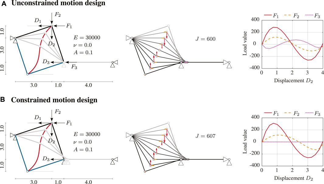
FIGURE 2. An illustrative example for unconstrained and constrained motion design. (A) Unconstrained motion design and (B) Constrained motion design.

Depending on the prescribed end-geometry, two different processes may be required:

• If only a part of the end-geometry is prescribed, the rest of the deformed geometry can adjust to meet equilibrium conditions. However, the maximum number of prescribed displacement degrees of freedom must be smaller than the number of allowed actuation forces.

• If the complete end-geometry is prescribed, then such configuration must be in equilibrium with the allowed actuation forces. If this is not possible, a new end-configuration is calculated through shape optimization before starting the motion design process. The objective of this shape optimization process is to obtain an end-configuration i.e., as close as possible to the desired end-configuration (minimizing the norm of the difference of node positions) subject to equilibrium constraints with the allowed actuation forces.

Figure 2B shows the solution obtained when no constrain on forces is applied. The motion path so obtained requires a total strain energy of J = 600. When only F₁ and F₂ are employed, the optimal deformation path so obtained requires a total strain energy of J = 607, which is larger compared to the unconstrained motion solution. When only one force is applied, no design variable (i.e., the relation between available actuation forces) is left for optimization, and thus the optimal deformation path reduces to that obtained from nonlinear structural analysis.

In addition to external actuation, which is modeled through external point forces, also internal actuation is considered by using linear actuators installed in series with structural elements (Sachse et al., 2021). An actuator element formulation is employed that is based on a bar element (tension/compression) but includes an additional parameter for the length change. A linear actuator can expand and contract its length. The total strain E_d of an actuator element is divided into two parts: the elastic strain E_el and the actuation strain E_act:

$E_d=E_{el}+E_{act}.(8)$

The actuation strain is not calculated from displacement values, but on the basis of a length change.

$l_{\alpha }=\left(1+\alpha \right)L.(9)$

The parameter α indicates the percentage of actuator length change, i.e., a value of α = 0.5 results in 50% elongation for an actuator with free-free boundary conditions.

Motion Through External Actuation

In the constrained motion design method outlined in Motion Design of Structures With Constraints, the locations of actuation forces are predetermined. Reducing the number of actuation forces to control the structure deformation path, generally, results in an increase of the integrated strain energy. An optimization problem is formulated to minimize such an increase of the integrated strain energy through optimal placement of external actuators. In this context the actuation forces are external point forces applied to the structure, i.e., the actuators are not included in the structure.

Efficient Placement of External Actuators

The calculation of an optimal set of actuation force locations is a discrete optimization problem. Due to a large number of possible combinations, a brute force approach is often not feasible. Depending on the problem formulation, various optimization methods could be applied to obtain a solution, such as genetic algorithms, mixed-integer programming, heuristic algorithms and gradient-based optimization algorithms of first and second order. The focus of this work is not on obtaining a global optimum of the actuator placement problem but rather a heuristic that can be conveniently employed with the constrained motion design method. A simple inverse greedy method that was first introduced in Kruskal (1956) and later used in Wagner et al. (2018) is adopted. The objective is to identify a feasible set of actuation force locations to control the structure through an optimal deformation path obtained by motion design. This inverse greedy algorithm is a robust heuristic that can be implemented with little effort. However, this algorithm cannot guarantee global optimality. Since the examples presented in this work are simple, solution quality can be assessed through a brute force search.

All possible actuation force locations are first considered, i.e., an unconstrained motion design is performed. The resulting unconstrained optimized motion serves as a predictor for a subsequent application of constrained motion design. Using the inverse greedy algorithm, the point forces are removed one by one and a constrained motion design is carried out for each force removal. The point force that causes the smallest increase of the objective function (strain energy integrated over the motion path) is removed from the set of applied actuation forces. Enough actuators are assumed to be available in order to reach the prescribed end displacement values exactly. This process is repeated until the desired number of actuation forces is reached. A flowchart of the actuator placement optimization process is given in Figure 3.

FIGURE 3

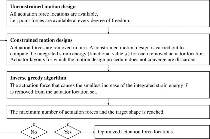
FIGURE 3. Flowchart of the actuator placement optimization algorithm.

An illustrative example of a statically indeterminate extended two-bar truss is given in Figure 4A. Two shallow arches are connected by a stiff element that is modeled with a larger cross-section area. The upper midpoint is to be moved downwards, i.e., its vertical displacement is prescribed. There are four free degrees of freedom in total, the horizontal and vertical degrees of freedom located at the upper and lower midpoint, respectively. First, an unconstrained motion design is carried out and an optimized motion path is obtained that requires integrated strain energy of J = 1,617. In this case, the upper node first rotates around the lower node and is then further moved downwards. This way, the large stiffness element is subjected to minimum strain, which avoids a significant increase of integrated strain energy. This deformation path requires all four actuation forces, as seen in Figure 4B1. It can be noted that although the problem description is symmetric, unsymmetric motion is obtained minimizing the integrated strain energy.

FIGURE 4

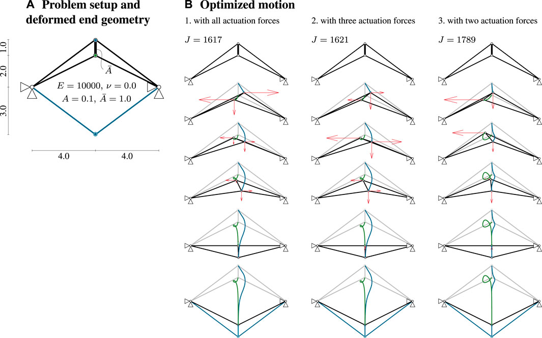
FIGURE 4. External actuation force placement in an extended two-bar truss. (A) Problem setup amd deformed end geometry. (B) Optimized motion, 1) with all actuation forces, 2) with three actuation forces, and 3) with two actuation forces.

Applying the inverse greedy algorithm, each actuation force is removed separately and a constrained motion design is carried out for each removal. The actuation force that causes the least deterioration of the functional value is then removed from the available actuation locations. In this example, the vertical force at the lower node has the least influence on the strain energy. By removing this force location, the integrated strain energy increases from J = 1,617 to J = 1,621, which is less than a 1% difference. The resulting motion is illustrated in Figure 4B2. The motion and the trajectory of both midpoints during deformation do not change significantly although only three forces instead of four forces are applied. This process repeats for the three remaining actuation force locations. In this second iteration, a more significant change can be observed in the trajectory of the two moving points, as shown in Figure 4B3. Also, the integrated strain energy increases to J = 1789 by approximately 11% compared to the unconstrained motion design. However, the overall motion path remains similar. The prescribed displacement values are reached exactly as their number is less than or equal to the number of actuation forces.

This example has shown that through the inverse greedy algorithm it is possible to identify the location of external actuation forces to perform an efficient motion between two prescribed geometries. This way, it is possible to further reduce the integrated strain energy compared to that required for a motion obtained with a predefined set of actuation force locations (as in Sachse et al., 2021).

Influence of the Prescribed End-Geometry

As explained in Motion Design of Structures With Constraints, it is possible to either fully prescribe the end-geometry or only parts of it. This choice has a significant influence on the actuator placement solution. Consider the simply supported truss example shown in Figure 5A. The structure is modeled with bar elements (black). The objective is to move the free top-chord nodes upwards. The end-geometry is defined as the deformed configuration that is computed through geometrically nonlinear analysis by applying a force F = 200 to each free top-chord node simultaneously.

FIGURE 5

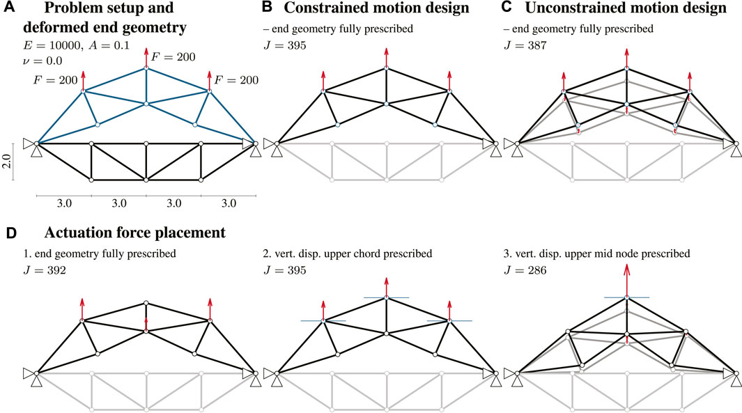
FIGURE 5. Influence of the end-geometry on actuator placement. (A) Problem setup amd deformed end geometry. (B) Constrained motion design. (C) Unconstrained motion design. (D) Acuation force motion, 1) end geometry fully prescribed, 2) vert. disp. upper chord prescribed, and 3) vert. disp. upper mid node prescribed.

A motion path discretization with eight linear elements is chosen and the vertical displacement of the upper mid node is controlled. In order to obtain reference solutions, a constrained motion design and an unconstrained motion design with a specification of the entire end-geometry are performed. The solution obtained through constrained motion design using three vertical forces involves a simultaneous increase of the actuation forces during motion (see Figure 5B) and requires an integrated strain energy J = 395. This motion path is similar to that obtained through a nonlinear analysis during which the force applied to each node is increased simultaneously. In the unconstrained motion design (Figure 5C), the same end-configuration is reached. This happens because the end-configuration is fully prescribed and has been determined through analysis. However, additional forces are applied during the deformation process to enable a more efficient motion that requires lower strain energy. Accordingly, before reaching the end-geometry, the deformation path goes through an intermediate configuration where additional actuation forces are applied. This leads to a reduction of integrated strain energy from J = 395 for the constrained motion design solution to J = 387 for the unconstrained motion design solution.

To study the influence of the prescribed end-geometry, three different cases are investigated that differ in the number of prescribed displacement values.

1. Figure 5D1: the end-geometry is fully prescribed. In this case, since the number of prescribed displacements is higher than the number of actuators, it is in general not possible to reach equilibrium in the target shape. For this reason, shape optimization is carried out before motion design (see Constrained Motion Design With a Prescribed Number of Actuators). Through shape optimization, a deformation state is obtained that is close to the desired end-geometry and in equilibrium with the current actuation forces. This leads to slightly modified end-geometries for each inverse greedy step. As a result, the final end-geometry can be realized through different actuation forces as those initially considered and it requires integrated strain energy J = 392, which is slightly lower than that required for case B.

2. Figure 5D2: only a part of the end-geometry is prescribed, in this case the vertical position of the upper chord nodes. The same actuation forces as in case B result from actuation placement optimization. The strain energy required in this case is identical to that for case B. In this case, the number of prescribed displacements and actuation forces is identical. As only some displacements are prescribed and not the entire end-geometry, these values are strictly enforced. Hence, actuation forces in other locations cannot control the structure into the prescribed end displacements and thus the solution is identical to that for case B.

3. Figure 5D3: a lower number of displacements than actuation forces is prescribed. In this case, only the vertical displacement of the upper mid node is specified. This way, further end-geometry variations and thus actuation force combinations are possible. A different end-geometry that requires significantly lower integrated strain energy J = 286 is obtained.

As expected, the prescribed end-geometry strongly influences the resulting actuation forces. In general, when more displacement values than available actuation forces are prescribed, shape optimization is employed to obtain a slightly different but feasible end-configuration that might require different actuation force locations compared to those initially assigned (Figure 5D1). When the prescribed number of displacements is equal to or lower than the available number of actuators, the prescribed end-configuration can be met exactly (Figure 5D2). Depending on design requirements, in order to reduce the integrated strain energy, the lowest number of displacements should be prescribed.

Morphing Cantilever

A morphing cantilever example is taken into consideration. The initial state is a hook-shaped configuration. The objective is to identify an efficient deformation path so that the free end-nodes reach the prescribed locations, as illustrated in Figure 6A. Motion is controlled through four actuation forces. The cantilever, which is fixed at the bottom, is modeled with 16 displacement-based plane four-node elements. The path is discretized with 18 linear elements.

FIGURE 6

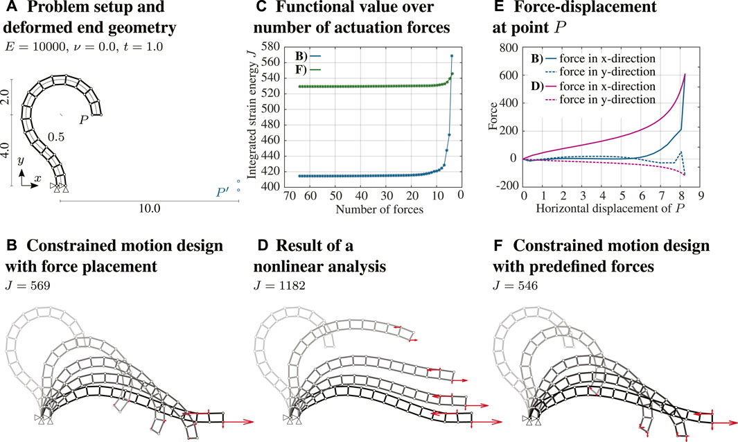
FIGURE 6. Motion design and actuation force placement for a morphing cantilever. (A) Problem setup amd deformed end geometry. (B) Constrained motion design with force placement. (C) Functional value over number of actuation forces. (D) Result of non-linear analysis. (E) Force displacement point P. (F) Constrained motion design with predefined forces.

First, an unconstrained motion design is carried out, whereby a deformation path is obtained so that the end-shape matches with the prescribed end-displacements. At this stage, all actuation forces are applied (Basic Method of Motion Design). The solution of this first process is given as starting point, i.e., a predictor motion, for a subsequent application of constrained motion design (Constrained Motion Design With a Prescribed Number of Actuators). In this second step, the motion is controlled through only four actuation forces, and therefore equilibrium constraints must be enforced throughout. The actuation force locations are identified through the placement method based on the inverse greedy algorithm (Efficient Placement of External Actuators). The solution of this second step is the location of the actuation forces as well as the deformation path enabled through such forces, as illustrated in Figure 6B. The four actuation forces are located at two nodes. The evolution of these four actuation forces throughout the deformation process is an output of motion design. The integrated strain energy required for this motion path is J = 569. The diagram in Figure 6C shows how the integrated strain energy varies as the actuation forces are removed (inverse greedy algorithm). This solution is compared to the result of a geometrically nonlinear analysis that is carried out by applying the same actuation forces obtained in B. Although the end-geometry is identical in both cases, the deformation path is dissimilar (cf. Figure 6D) because actuation forces are applied differently throughout the motion. In a geometrically nonlinear analysis, all forces are increased simultaneously and uniformly, whereas, through motion design, actuation forces are varied independently or simultaneously as required. This effect can be observed in the force-displacement diagram shown in Figure 6E, where the horizontal and vertical forces at point P are plotted over the horizontal displacement. When the end-geometry is reached, the force-displacement curves come together to the same point. The deformation caused by a uniform increase of forces results in integrated strain energy J = 1,182, which is significantly larger than that required through motion design.

Another approach to identifying efficient actuation force locations is to consider the location set that requires the lowest strain energy in the deformed end-state. This approach does not consider the entire motion, but it minimizes the strain energy in the end-configuration. Consequently, another set of actuation forces is obtained. This solution is illustrated in Figure 6F. The motion path is similar to that of case B. Although the end-geometry varies slightly, the prescribed two free end-node locations are satisfied. The strain energy required in this case is lower than the energy required by the solution of motion design in case B. To compare both approaches, the evolution of integrated strain energy as the point forces are successively removed (in an inverse greedy algorithm scheme) until the prescribed set of four forces remains, is illustrated in Figure 6C. The end-geometry in this second approach requires lower strain energy. However, all other force location combinations that include more than four actuators, require larger strain energy for case F (cf. Figure 6B). Owing to the inability of the inverse greedy algorithm to guarantee solution optimality, the location of some of the forces considered in case F has been removed during the optimization process, which explains the larger integrated strain energy for case B when the number of actuator forces is reduced to four. That being said, both approaches give a good estimation of an efficient motion design and actuation force placement.

Motion Through Internal Actuation

Elastic and Actuation Energy

In previous examples, the motion path has been controlled through external actuation forces. However, also internal actuators can be employed. Internal actuator elements are modeled using the formulation given in Sachse et al. (2021) that has been summarized in Constrained Motion Design With a Prescribed Number of Actuators. In this formulation, the intended actuator length change is treated as an additional variable of the motion design process. The actuator length changes are varied to control the structure into the required deformation path. The optimal deformation path and actuator length changes are outputs of motion design. In previous examples, the objective has been the minimization of strain energy integrated over the deformation path. However, as presented in Sachse and Bischoff (2020), other objectives can be employed, such as integrated stress or strain of the entire structure or only parts of it. The total strain energy is defined as

${\mathrm{\Pi }}_{\mathrm{int}}\mathrm{=}{\displaystyle {\int }_{\mathrm{\Omega }}\frac{\mathrm{1}}{\mathrm{2}}{\mathbf{S}}^{\mathrm{T}}\left({\mathbf{E}}_{\mathrm{el}}\mathrm{+}{\mathbf{E}}_{\mathrm{act}}\right)\mathrm{d\Omega }}\mathrm{=}{\displaystyle {\int }_{\mathrm{\Omega }}\frac{\mathrm{1}}{\mathrm{2}}{\mathbf{E}}_{\mathrm{el}}^{\mathrm{T}}\mathbf{C}\left({\mathbf{E}}_{\mathrm{el}}\mathrm{+}{\mathbf{E}}_{\mathrm{act}}\right)}\mathrm{d\Omega =}{\displaystyle {\int }_{\mathrm{\Omega }}\left(\frac{\mathrm{1}}{\mathrm{2}}{\mathbf{E}}_{\mathrm{el}}^{\mathrm{T}}\mathbf{C}{\mathbf{E}}_{\mathrm{el}}\mathrm{+}\frac{\mathrm{1}}{\mathrm{2}}{\mathbf{E}}_{\mathrm{el}}^{\mathrm{T}}\mathbf{C}{\mathbf{E}}_{\mathrm{act}}\right)\mathrm{d\Omega }}(10)$

where $\mathbf{S}$ is the element stress and E is the total strain which is divided into the elastic strain E_el and the strain due to actuation E_act. The elastic energy is defined as

${\text{Π}}_{\text{int},\text{el}}=\underset{\text{Ω}}{{\displaystyle \int }}\frac{1}{2}{\mathbf{E}}_{\text{el}}^T\mathbf{C}{\mathbf{E}}_{\text{el}}\text{dΩ}(11)$

while the actuation energy is

${\text{Π}}_{\text{int},\text{act}}=\underset{\text{Ω}}{{\displaystyle \int }}\frac{1}{2}{\mathbf{E}}_{\text{el}}^T\mathbf{C}{\mathbf{E}}_{\text{act}}^T\text{dΩ}.(12)$

In practice, even when the actuator moves under no force, a length change requires input energy, which could be included via an extra term in the actuation energy in Equation 12. However, this depends on the type of actuation technology. In the case of external actuation, the elastic energy is the total strain energy. In the general case, both energy shares are integrated over the deformation path and are a measure of the cost of deformation. Depending on the problem and application, either of them may be used.

The actuation energy given in Eq. 12 does not differentiate between positive and negative actuation work. In other words, it is possible that through the deformation path, some of the elastic energy stored in a previous control step is released, because the model allows for energy harvesting. If energy harvesting is not possible, this formulation might lead to an underestimation of the actuation energy that is required to control the structure through the optimal deformation path. To avoid energy gains during motion, the objective function should become a discontinuous function as formulated in Senatore and Reksowardojo (2020), which, in this case, since large deformations are considered, would make the optimization formulation significantly more complex.

To reduce optimization complexity, in this work only the first energy share (elastic) is considered.

Efficient Placement of Internal Actuators

The location of internal actuators is sought to control the structure through the optimal deformation path using minimum elastic energy. For simplicity, only truss structures are investigated. The same example as that described in Influence of the Prescribed End-Geometry (Figure 5) is taken as a case study. The influence of different degrees of static indeterminacy is tested by adding two and four bars, which results in a degree of static indeterminacy of three and five, respectively. The specification of the end-geometry is carried out by prescribing one (as in Figure 5D2) and three end-displacements (as in Figure 5D3). As for the optimization of external actuator forces (Efficient Placement of External Actuators), it is assumed that enough actuators are available to reach the prescribed end-displacements exactly.

There are two ways to model internal actuators. Actuators can be installed in series and parallel with a truss element. With regard to parallel actuation, an actuator element is added in the same location of a truss element. Consequently, both elements are connected at the nodes and when the actuator element changes length, the truss element must also change length through deformation, which creates a resisting force. With regard to serial actuation as considered in this work, the actuator replaces (entirely or partially) a truss element. In this case, the actuator length change does not cause a deformation in a hosting truss element. However, deformation can still occur in the hosting element owing to resisting forces that develop through the stiffness of the rest of the structure.

Referring to the optimization method employed for the placement of external actuators (Efficient Placement of External Actuators), the application of an inverse greedy algorithm for internal actuator placement would require replacing all elements with actuators in the first step. In such a case, assuming that each actuator replaces its hosting element entirely, there would be no resistance from passive elements. Since the objective is the minimization of integrated elastic energy (no actuation energy is accounted for) and no stress/stability constraints are enforced, the motion design problem becomes highly ill-posed i.e., infinite optimal motion paths exist to reach the target geometry. Therefore, to avoid convergence issues, the optimal actuator placement is carried out by adopting a brute force search combined with a greedy algorithm, whereby actuators are added one by one in turn:

- Step 1: The number of actuators is progressively increased and all combinations are tested until the specified end-displacements are met.

- Step 2: If there are enough actuators such that the end-displacement specifications can be met, the combination that requires the lowest elastic energy is selected.

- Step 3: In case more actuators are considered, the solution obtained in step 2 is employed as a basis. The remaining truss elements are replaced by actuators in turn. The actuator location combination that results in the smallest functional value is selected. This step of the greedy algorithm is repeated until the desired number of actuators is reached.

An optimal actuator placement is sought that minimizes the elastic energy integrated over the motion path. Two cases are analyzed in the following. First, the minimum number and location of actuators are determined in order to reach the specified end-geometry through a finite mechanism. Second, an optimal placement of actuators is determined to reach the end-geometry through a deformation path that requires minimum elastic energy.

Minimum Number of Actuators to Enable Motion Through Finite Mechanisms

When a certain number of actuators replace truss elements a motion path through finite mechanisms can be identified that requires minimal (zero) strain energy (energy loss due to friction is not considered). However, whether such finite mechanisms exist depends on the structural topology, the degree of static indeterminacy n_s, the number and location of the actuators as well as the number of prescribed displacements of the end-configuration. The number of actuators required to enable motion through a finite mechanism is calculated within step 1 of the algorithm for efficient placement of internal actuators (Efficient Placement of Internal Actuators). The number of actuators is gradually increased and all combinations are tested until the prescribed end-displacements are reached through a finite mechanism which is identified when the integrated elastic energy is zero. Often there exist several actuator location combinations that enable motion through a finite mechanism. Figure 7 shows finite mechanisms resulting from actuator placement for three different structures, which differ in the degree of their static indeterminacy, n_s = 1, n_s = 3 or n_s = 5.

FIGURE 7

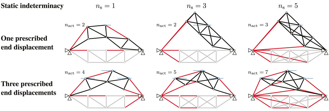
FIGURE 7. Examples of internal actuator locations (marked in red) that enable motion through a finite mechanism. (A) Static indeterminacy. (B) One prescribed end displacement. (C) Three prescribed end displacement.

In all examples, the length of truss elements that are not replaced by actuators remains identical in the initial and end-geometry. Therefore, the elastic energy is zero and thus an elastic-energy-free motion is possible. The minimum number of actuators n_act to enable such a motion depends on the structure topology and the prescribed end-displacements. For example, when only one end-displacement is prescribed, two actuators are needed for the first two topology examples even though the degree of static indeterminacy n_s is different. For the structure with n_s = 5, one additional actuator, i.e., three actuators are needed. In general, the more displacement values are prescribed, the more actuators are required. However, the actuator layout for a specific number of actuators n_act to enable a finite mechanism is not unique. Examples of possible actuator layouts are illustrated in Figure 7. There exist other actuator location combinations that fulfill the defined requirements.

Actuator Placement for Motion Through Deformation

If there are not enough actuators available to enable motion through finite mechanisms, the actuator locations can be selected based on their contribution to control the structure through the required deformation path using minimum elastic energy. The algorithm for efficient placement of internal actuators (Efficient Placement of Internal Actuators) is applied. An illustrative example is given in Figure 8. Three displacement values are prescribed and the degree of statistical indeterminacy is n_s = 3. The result of step 2 is shown in Figure 8A. The end-displacements are reached exactly using three actuators. From all combinations of three actuators (only some combinations are shown in Figure 8), the placement that results in the elastic energy integrated over the motion path (J = 135) is chosen. Starting from this configuration, one additional truss element is replaced by an actuator, and a new actuator layout is obtained which requires lower integrated elastic energy as shown in Figure 8B.

FIGURE 8

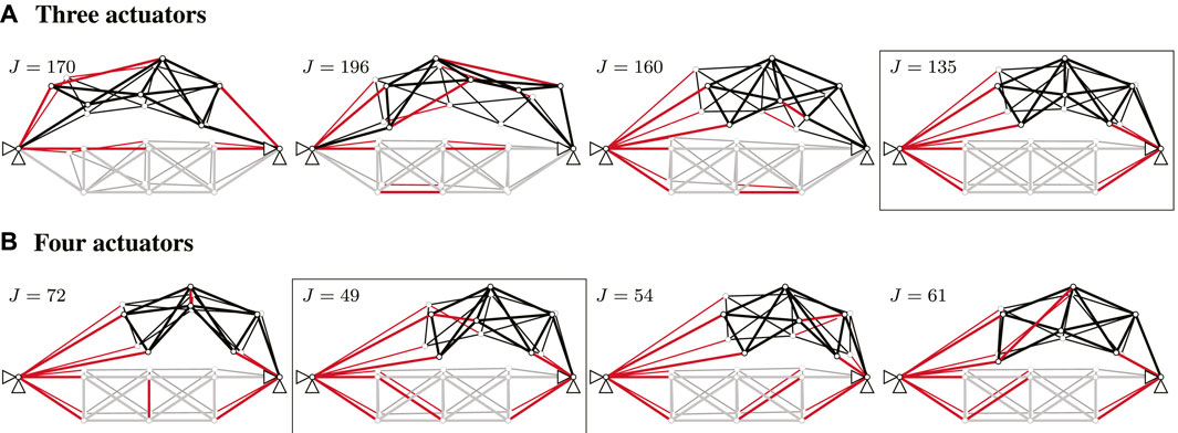
FIGURE 8. Actuator placement for elastic energy minimization. (A) Three actuators. (B) Four actuators.

Discussion

This work has presented an extension of previous methods for motion design through a combination of heuristic algorithms for actuator placement. The methods presented in this paper are useful to identify a subset of external or internal actuator force locations that enable control of the structure through a required motion path between two significantly different geometric configurations. This work has focused on actuator placement through minimization of the elastic energy integrated over the motion path. No quantification of the actuation energy has been investigated. However, minimization of the integrated actuation energy in Eq. 12 can also be used to obtain suitable actuator placements. The choice of objective function depends on the intended application. If large element deformations must be prevented, minimization of the elastic energy should be employed. On the other hand, minimization of actuation energy could be chosen when control of the motion path requires large actuation energy. Future work could look into the quantification of actuator energy and testing different actuation technologies.

An inverse greedy algorithm has been applied to identify optimal locations of external actuators. This algorithm cannot guarantee global optimality, i.e., important actuation force locations may be excluded early in the optimization process. A combination of brute force and a greedy algorithm has been employed for the placement of internal actuators. Similar limitations regarding solution quality apply in this case. Owing to the iterative nature of motion design and its sequential application in combination with the heuristics adopted for actuator placement, the overall procedure has a high computational cost. The overall number of iterations can be reduced by using the solution obtained from a previous motion design as a predictor (i.e., starting configuration) for a subsequent iterative cycle. This reduces the overall computation time compared to a single motion design that starts from a naïve predictor (e.g., linear interpolation). Future work could look into implementing different algorithms that are better suited for large-scale numerical optimization.

The presented work has aimed to evaluate the application feasibility of the proposed motion design method through numerical examples. Making this method more relevant to practical applications will be the subject of future work. Among possible extensions, constraints on actuation could be added, for example, to limit the actuator length changes. In addition, constraints on material strength, structural element stability should be added to ensure that structural integrity is preserved throughout motion. The proposed method is also suitable to identify inextensible deformations of shells, which could be employed to control large geometry changes with low control effort.

Conclusion

The method of motion design has been successfully combined with heuristic algorithms for optimal actuator placement. While the heuristics implemented in this work do not guarantee global optimality, they generally allow the identification of efficient actuator layouts that enable control of the structure through the required motion path.

Constrained motion design is able to identify motion paths that are more efficient than those obtained from intuitive approaches. Numerical simulations have shown that strategically restricting actuation to a limited number of locations (i.e., degrees of freedom) does not significantly change the overall motion path obtained with unconstrained motion design. A naïve proportional increase of actuation forces to control the structure into a given target configuration requires a significantly larger cost of deformation (i.e., indication of control energy) than that required by a motion design solution. This is because the motion design method takes into account the entire deformation process, not only the final configuration. Generally, as expected, the fewer displacement values of the end-geometry are prescribed, the lower the cost of deformation.

Data Availability Statement

The original contributions presented in the study are included in the article, further inquiries can be directed to the corresponding author.

Author Contributions

RS did the development of the method and the investigation under a close guidance by MB and assistance of FG and MV.

Funding

This research work by RS was part of the collaborative project “Bio-inspirierte Materialsysteme and Verbundkomponenten fur nachhaltiges Bauen im 21ten Jahrhundert” (BioElast) funded by the State¨ Ministry of Baden-Wuerttemberg for Sciences, Research and Arts. Furthermore, the contribution of FG was conducted in the framework of the Collaborative Research Center 1244 “Adaptive Skins and Structures for the Built Environment of Tomorrow”/project B01 funded by the Deutsche Forschungsgemeinschaft (DFG, German Research Foundation)—project number 279064222. The authors are grateful for the generous support.

Conflict of Interest

The authors declare that the research was conducted in the absence of any commercial or financial relationships that could be construed as a potential conflict of interest.

References

Abdullah, M. M., Richardson, A., and Hanif, J. (2001). Placement of Sensors/actuators on Civil Structures Using Genetic Algorithms. Earthquake Engng. Struct. Dyn. 30, 1167–1184. doi:10.1002/eqe.57

CrossRef Full Text | Google Scholar

Gupta, V., Sharma, M., and Thakur, N. (2010). Optimization Criteria for Optimal Placement of Piezoelectric Sensors and Actuators on a Smart Structure: A Technical Review. J. Intell. Mater. Syst. Structures 21, 1227–1243. doi:10.1177/1045389x10381659

CrossRef Full Text | Google Scholar

Hasse, A., and Campanile, L. F. (2009). Design of Compliant Mechanisms with Selective Compliance. Smart Mater. Struct. 18, 115016. doi:10.1088/0964-1726/18/11/115016

CrossRef Full Text | Google Scholar

Ibrahimbegovic, A., Knopf-Lenoir, C., Kuerov̌, A., and Villon, P. (2004). Optimal Design and Optimal Control of Structures Undergoing Finite Rotations and Elastic Deformations. Int. J. Numer. Meth. Engng. 61, 2428–2460. doi:10.1002/nme.1150

CrossRef Full Text | Google Scholar

Inoue, F. (2008). “Development of Adaptive Construction Structure by Variable Geometry Truss,” in Robotics and Automation in Construction. Editors C. Balaguer, and M. Abderrahim (London, United Kingdom: InTech)). doi:10.5772/5543

CrossRef Full Text | Google Scholar

Irschik, H. (2002). A Review on Static and Dynamic Shape Control of Structures by Piezoelectric Actuation. Eng. Structures 24, 5–11. doi:10.1016/s0141-0296(01)00081-5

CrossRef Full Text | Google Scholar

Jani, J. M., Leary, M., Subic, A., and Gibson, M. A. (2014). A Review of Shape Memory alloy Research, Applications and Opportunities. Mater. Des. (1980-2015) 56, 1078–1113. doi:10.1016/j.matdes.2013.11.084

CrossRef Full Text | Google Scholar

Knippers, J., and Schlaich, J. (2000). Folding Mechanism of the Kiel Hörn Footbridge, Germany. Struct. Eng. Int. 10, 50–53. doi:10.2749/101686600780620991

CrossRef Full Text | Google Scholar

Knippers, J., Jungjohann, H., Scheible, F., and Oppe, M. (2013). Bio-inspirierte kinetische Fassade für den Themenpavillon "One Ocean" EXPO 2012 in Yeosu, Korea. Bautechnik 90 (6), 341–347. doi:10.1002/bate.201300034

CrossRef Full Text | Google Scholar

Kota, S., Joo, J., Li, Z., Rodgers, S. M., and Sniegowski, J. (2001). Design of Compliant Mechanisms: Applications to MEMS. Analog Integrated Circuits Signal. Process. 29, 7–15. doi:10.1023/a:1011265810471

CrossRef Full Text | Google Scholar

Kruskal, J. B. (1956). On the Shortest Spanning Subtree of a Graph and the Traveling Salesman Problem. Proc. Amer. Math. Soc. 7, 48. doi:10.1090/s0002-9939-1956-0078686-7

CrossRef Full Text | Google Scholar

Kwan, A. S. K., and Pellegrino, S. (1993). Prestressing a Space Structure. AIAA J. 31, 1961–1963. doi:10.2514/3.11876

CrossRef Full Text | Google Scholar

Masching, H., and Bletzinger, K.-U. (2016). Parameter Free Structural Optimization Applied to the Shape Optimization of Smart Structures. Finite Elem. Anal. Des. 111, 33–45. doi:10.1016/j.finel.2015.12.008

CrossRef Full Text | Google Scholar

Masic, M., and Skelton, R. E. (2005). Path Planning and Open-Loop Shape Control of Modular Tensegrity Structures. J. Guidance, Control Dyn. 28, 421–430. doi:10.2514/1.6872

CrossRef Full Text | Google Scholar

Preumont, A. (2011). Vibration Control of Active Structures: An Introduction. Solid Mechanics and its Applications. 3 edn. Dordrecht: Springer Netherlands. doi:10.1007/978-94-007-2033-6

CrossRef Full Text

Reksowardojo, A. P., Senatore, G., and Smith, I. F. C. (2019). Experimental Testing of a Small-Scale Truss Beam that Adapts to Loads through Large Shape Changes. Front. Built Environ. 5, 93. doi:10.3389/fbuil.2019.00093

CrossRef Full Text | Google Scholar

Reksowardojo, A. P., Senatore, G., and Smith, I. F. C. (2020). Design of Structures that Adapt to Loads through Large Shape Changes. J. Struct. Eng. 146, 04020068. doi:10.1061/(asce)st.1943-541x.0002604

CrossRef Full Text | Google Scholar

Sachse, R., and Bischoff, M. (2020). A Variational Formulation for Motion Design of Adaptive Compliant Structures. Int. J. Numer. Methods Eng. 122, 972–1000. doi:10.1002/nme.6570

CrossRef Full Text | Google Scholar

Sachse, R., Geiger, F., and Bischoff, M. (2021). Constrained Motion Design with Distinct Actuators and Motion Stabilization. Int. J. Numer. Methods Eng. 122, 2712–2732. doi:10.1002/nme.6638

CrossRef Full Text | Google Scholar

Senatore, G., and Reksowardojo, A. P. (2020). Force and Shape Control Strategies for Minimum Energy Adaptive Structures. Front. Built Environ. 6, 105. doi:10.3389/fbuil.2020.00105

CrossRef Full Text | Google Scholar

Senatore, G., Duffour, P., Winslow, P., and Wise, C. (2018). Shape Control and Whole-Life Energy Assessment of an ‘infinitely Stiff’ Prototype Adaptive Structure. Smart Mater. Structures 27, 015022. doi:10.1088/1361-665x/aa8cb8

CrossRef Full Text | Google Scholar

Senatore, G., Duffour, P., and Winslow, P. (2019). Synthesis of Minimum Energy Adaptive Structures. Struct. Multidisc Optim 60 (3), 849–877. doi:10.1007/s00158-019-02224-8

CrossRef Full Text | Google Scholar

Seok, S., Wang, A., Meng Yee Chuah, M. Y., Otten, D., Lang, J., and Kim, S. (2013). Design Principles for Highly Efficient Quadrupeds and Implementation on the MIT Cheetah Robot, 2013. Karlsruhe, Germany: IEEE International Conference on Robotics and Automation, 3307–3312. doi:10.1109/ICRA.2013.6631038

CrossRef Full Text

Sobek, W., and Teuffel, P. (2001). “Adaptive Systems in Architecture and Structural Engineering,” in Smart Structures and Materials 2001: Smart Systems for Bridges, Structures, and Highways, 4330. Bellingham, Washington: International Society for Optics and Photonics, 36–46.

Google Scholar

Sofla, A. Y. N., Elzey, D. M., and Wadley, H. N. G. (2009). Shape Morphing Hinged Truss Structures. Smart Mater. Structures 18, 065012. doi:10.1088/0964-1726/18/6/065012

CrossRef Full Text | Google Scholar

Sychterz, A. C., and Smith, I. F. C. (2018). Deployment and Shape Change of a Tensegrity Structure Using Path-Planning and Feedback Control. Front. Built Environ. 4, 45. doi:10.3389/fbuil.2018.00045

CrossRef Full Text | Google Scholar

Teuffel, P. (2004). Entwerfen Adaptiver Strukturen. Stuttgart: Ph.D. thesis, University of Stuttgart. doi:10.2749/222137804796302004

CrossRef Full Text

Veuve, N., Sychterz, A. C., and Smith, I. F. C. (2017). Adaptive Control of a Deployable Tensegrity Structure. Eng. Structures 152, 14–23. doi:10.1016/j.engstruct.2017.08.062

CrossRef Full Text | Google Scholar

Wagner, J. L., Gade, J., Heidingsfeld, M., Geiger, F., von Scheven, M., Böhm, M., et al. (2018). On Steady-State Disturbance Compensability for Actuator Placement in Adaptive Structures. at Automatisierungstechnik 66, 591–603. doi:10.1515/auto-2017-0099

CrossRef Full Text | Google Scholar

Wang, Y., and Senatore, G. (2020). Minimum Energy Adaptive Structures - All-In-One Problem Formulation. Comput. Structures, vol. 236, p. 106266. doi:10.1016/j.compstruc.2020.106266

CrossRef Full Text | Google Scholar

Wijdeven, J. v. d., and Jager, B. d. (2005). “Shape Change of Tensegrity Structures: Design and Control,” in Proceedings of the 2005, 4, Portland, OR: American Control Conference. 2522–2527.

Google Scholar