Performance Assessment of Metaheuristic Algorithms for Structural Optimization Taking Into Account the Influence of Algorithmic Control Parameters

1 Introduction

Metaheuristic algorithms are widespread in the literature on discrete and combinatorial optimization. They operate by applying stochastic (as opposed to deterministic) operators to explore the design space and to guide the search toward optimal designs, implying the need for statistical techniques to properly assess their performance. Nowadays, formal statistical analysis is considered a prerequisite for papers on non-deterministic optimization algorithms (Le Riche and Haftka, 2012; Haftka, 2016).

Metaheuristic algorithms are typically controlled by a number of algorithmic parameters, which can be modified to tune the search procedure to the optimization problem at hand. These parameters are referred to as control parameters in this article. The performance of a metaheuristic algorithm depends on three factors: 1) the specific optimization problem at hand, 2) the values of the control parameters, and 3) the random variability inherent to stochastic algorithms.

In the structural optimization community, it is common practice to benchmark newly proposed algorithms against one or more reference algorithms in order to assess their performance. Such benchmark studies are usually based on a simulation in which multiple optimization runs are performed (to compensate for the effect of the random seed) on a series of representative test problems (to compensate for the effect of the optimization problem). However, the effect of the control parameters is mostly ignored: their values are either chosen by intuition or convention, taken from other studies, or motivated by ad hoc experimentation, usually limited to changing one parameter value at a time (Chiarandini et al., 2007). From that moment on they remain fixed, although Bartz-Beielstein (2006) has shown that conclusions regarding algorithm performance do not necessarily apply to other parameter values.

Considering the wide range of metaheuristic algorithms currently in use, it is important to be able to assess their performance in an objective manner. For example, in a benchmarking context it would be fair to tune the control parameter values of all algorithms under consideration—using comparable resources—before moving on to the actual comparison (Eiben and Smit, 2011). Moreover, data on optimal control parameter values across multiple studies might reveal search strategies that work particularly well for a specific kind of optimization problem. In this regard, Hooker (1995) made the distinction between competitive and scientific testing, which, in the context of metaheuristic algorithms, is still very relevant today. Besides finding out which algorithm is better (competitive testing), it is important to investigate why this is the case (scientific testing). Hooker describes the former as “anti-intellectual,” as he believes that the emphasis on competition does not contribute to the sort of insight that will lead to the development of better algorithms in the long run.

Various methods exist to assess the performance of metaheuristic algorithms, including performance profiles (Dolan and Moré, 2002), data profiles (Moré and Wild, 2009), a probabilistic performance metric based on the effect size in statistics (Gomes et al., 2018) and statistical analysis methods by e.g. Charalampakis and Tsiatas (2019) and Georgioudakis and Plevris (2020). However, these methods are rarely used in a structural optimization context and there is no consensus on which method to use instead. A common approach is to perform several independent runs of the algorithm and to summarize the results using descriptive statistics, but the number of different runs and the statistics reported vary from study to study.

There is a trend in metaheuristic optimization to either reduce the number of (external) control parameters, as for example in the Newton metaheuristic algorithm by Gholizadeh et al. (2020), or to develop algorithms that update their parameters on-the-go, although these often have fixed parameters as well (Hutter et al., 2009b). Whether this is beneficial depends on the robustness of the algorithm with respect to the control parameters. An algorithm with many control parameters, whose values have little effect on performance or can be easily selected using rules of thumb, may still be preferable to an algorithm with few control parameters that need careful tuning. Therefore, a good performance assessment method should integrate the sensitivity of the algorithm with respect to its control parameter configuration.

This article presents a new method, designed to assess the performance of a metaheuristic algorithm in relation to the values of its control parameters. The scope is limited to control parameters whose values are constant throughout the optimization. The method is based on Monte Carlo simulation. The general idea is to perform multiple optimization runs, where the values of the control parameters vary randomly. From the resulting dataset, a subset of well-performing runs (e.g. the 10% best) is studied. The occurrence frequency of the various parameter values in this subset indicates which parameter values give rise to good performance. The threshold for “good” performance is gradually tightened, making the results more relevant, but also less accurate, as the well-performing subset will contain fewer samples. An adaptive importance sampling technique is used to sample good parameter values more often, ensuring sufficient accuracy throughout the procedure.

The proposed method is mathematically rigorous and has the advantage of being able to process any number of control parameters, both numerical and categorical, at the same time, presenting the results in a visual and intuitive way. It is intended as a tool to help developers of metaheuristic algorithms to test and benchmark their algorithm. Four possible applications are given below.

• The method can be used to investigate the sensitivity of an algorithm with respect to the control parameters. It identifies parameters that do not have a significant effect on performance and detects well-performing parameter values for the important parameters, helping developers to focus on the relevant parts of their algorithm.

• The method can also be used to select appropriate default values for the control parameters of a new algorithm, similar to the way in which the optimal and the default matlab values are compared for the genetic algorithm in Section 4.

• The method records the probability of achieving different levels of performance when parameter values are randomly selected from a set of user-defined “reasonable” options. The results can be compared with other algorithms to make statements about the overall performance in case no good parameter values would be known and the parameter configuration would be chosen arbitrarily.

• As a by-product, the method may generate new benchmark results for the community, as evidenced by the improvement over the best known solution for two of the test cases in Section 4.

The remainder of the article is structured as follows. Section 2 gives an outline of the state of the art on parameter tuning methods, providing an overview of ways to account for the influence of the control parameters. Section 3 presents the problem definition and describes the proposed methodology. Section 4 presents two numerical experiments, based on the genetic algorithm that is built into matlab, for seven test problems that are commonly used in the structural optimization literature. Section 5 provides final conclusions.

2 State of the Art in Parameter Tuning

Automated parameter tuning is a well-studied problem in the field of computational intelligence and machine learning. The following paragraphs summarize the state of the art.

2.1 Early Work

Research on the influence of control parameters started not long after the introduction of genetic algorithms and was initially mainly theoretical. Examples include Bäck and Schwefel (1993) and Rechenberg (1973). However, such theoretical models were either overly complex or required severe simplifications, making them of limited use in practical settings (Myers and Hancock, 2001). It became customary to study the effect of the control parameters through experimentation, using empirical models to test different parameter settings. Some authors, such as De Jong (1975), attempted to formulate universally valid control parameter configurations, until the No Free Lunch theorems (Wolpert and Macready, 1997) shattered the illusion of finding parameter values that are universally applicable.

2.2 Meta-Optimization

Alternatively, automatic tuning methods have been studied that tune the parameters for a single specific problem. A popular example is meta-optimization, which follows from the observation that choosing control parameters for maximal performance is an optimization problem in itself. In the meta-level problem, the control parameters are the design variables, and the performance of the algorithm is the objective function (often called the performance landscape). Depending on the nature of the control parameters, the meta-level problem is a mixed variable stochastic optimization problem that can be solved for example by iterated local search (ParamILS by Hutter et al. (2009b)) or by another metaheuristic algorithm (Nannen and Eiben, 2007; Ansótegui et al., 2009). The meta-optimizer can be applied either directly to the performance landscape (Grefenstette, 1986) or to a surrogate model of it (Audet and Orban, 2004).

2.3 Design of Experiments, Model-Based Optimization and Machine Learning

A popular class of tuning methods is based on the principles of Design of Experiments (DOE), which aims to maximize the information obtained from experiments in highly empirical fields of science such as biology and psychology. Common approaches include factorial designs, coupled with analysis of variance or regression analysis, e.g. Adenso-Diaz and Laguna (2006), Coy et al. (2001) and Rardin and Uzsoy (2001). The DOE methodology was later replaced by the Design and Analysis of Computer Experiments (DACE) methodology (Sacks et al., 1989), specifically created for deterministic computer algorithms (Bartz-Beielstein et al., 2004). Bartz-Beielstein et al. (2005) introduced Sequential Parameter Optimization (SPO), which uses Kriging techniques to build a predictive model of the performance landscape based on an increasing number of observations that are selected through an expected improvement criterion. Hutter et al. (2009a), Hutter et al. (2010) gave suggestions to further improve the method. Hutter et al. (2011) later introduced Sequential Model-based Algorithm Configuration (SMAC), extending model-based approaches to categorical parameters and sets of multiple problem instances using random forests (collections of regression trees). Independently, Dobslaw (2010) combined the DOE methodology with artificial neural networks as a basis for a parameter tuning framework.

2.4 Model-free Algorithm Configuration

In a separate line of work, statistical hypothesis testing has been used to compare different control parameter settings, for example in Czarn et al. (2004), Castillo-Valdivieso et al. (2002) and Xu et al. (1998). In this approach, evidence is gathered on the basis of experimental runs to test whether the considered parameter settings show a difference in performance that is significant enough to be distinguishable from stochastic noise. Nevertheless, the number of experimental runs that is required for sufficient statistical accuracy is often quite large (Yuan and Gallagher, 2007). Birattari et al. (2002) presented an efficient alternative with the F-Race algorithm, which progressively tests a number of (predefined) parameter configurations on one or more benchmark problems and eliminates inferior ones as soon as significance arises. Balaprakash et al. (2007) presented two improvement strategies for the F-Race algorithm, called sampling design and iterative refinement, and Yuan and Gallagher (2007) proposed a combination of F-Race and meta-optimization. More recently, López-Ibáñez et al. (2016) presented the irace package, offering iterated racing with a restart mechanism to prevent premature convergence and elitist racing to ensure that the best parameter configurations are tested most thoroughly. Li et al. (2017) introduced Hyperband, formulating the parameter tuning problem as an infinite-armed bandit problem, adaptively allocating more resources to promising parameter configurations in order to enhance random search. Falkner et al. (2018) combined Hyperband with Bayesian optimization in the BOHB (Bayesian optimization and Hyperband) method.

2.5 Parameter Tuning in Structural Optimization

In a structural optimization context, research into parameter tuning has received little attention so far. However, there have been several studies on parameter control, where parameter values are updated during the optimization process. For a general overview of parameter control methods, the reader is referred to Karafotias et al. (2015). Examples of parameter control applied to structural optimization include Hasançebi (2008) for evolutionary strategies, Hasançebi et al. (2009) for harmony search, Nickabadi et al. (2011) for particle swarm optimization and Kaveh and Farhoudi (2011) for metaheuristic algorithms in general.

The present authors have recently proposed a new parameter tuning method for structural optimization (Dillen et al., 2018). The method uses Monte Carlo simulation to estimate the distribution of performance of a metaheuristic algorithm under the condition that control parameter x has value y. Although this method is able to correctly reflect the effect of the dominant control parameters, it has difficulty in coping with effects that are due to parameter interactions: if a particular value of one control parameter only performs well in combination with a particular value of another control parameter, this will not be detected by the method.

3 Problem Definition and Methodology

3.1 List of Symbols

Table 1 presents an overview of the symbols that are used in the text. By convention, vectors are represented by bold characters. A function $X\left(\theta \right)$ of θ that is denoted by an upper-case letter represents a random variable. The lower-case equivalent x represents a specific value of X. A hat means that the variable $\widehat{x}$ is an estimate of x. Finally, the subscript k or superscript (k) means that the variable is computed on the basis of the samples from the kth stage in the simulation.

TABLE 1

TABLE 1. List of symbols.

3.2 General Approach

The following paragraphs establish a solid mathematical basis for the performance assessment problem and continue with the derivation of a Monte Carlo estimator and an importance sampling estimator for the statistic of interest. Next, the relevant properties of ratio estimators are briefly discussed. After that, the characteristics of a good importance sampling distribution are described. Finally, a method is given to iteratively update the importance sampling distribution based on adaptive importance sampling.

3.3 Problem Definition

To model the uncertainty in the simulation, we introduce a probability space $\left(\text{Ω},\mathcal{S},\text{Pr}\right)$, where $\text{Ω}$ represents the sample space, $\mathcal{S}$ the set of events, and $\text{Pr}$ a probability measure that assigns probabilities to the events (Kolmogorov, 1956). The elements θ of $\text{Ω}$ are considered to be selected by the true randomness that underlies all natural processes. Each element θ corresponds to a unique state of the random problem.

Suppose we want to assess the performance of a metaheuristic algorithm $\mathcal{A}$ on an optimization problem $\mathcal{P}$. The outcome of a single run of the algorithm depends on the parameter configuration $\mathbf{p}={\left(p_1,p_2,\dots ,p_n\right)}^T$, and a random component $H\left(\theta \right)$ that is inherent to the class of metaheuristic algorithms¹. Each component of the parameter configuration vector $\mathbf{p}$ represents the value of a single control parameter. In this study, the value of $\mathbf{p}$ is considered to be a realization of an n-variate random vector $\mathbf{P}\left(\theta \right)$, where

$\theta \mapsto \mathbf{P}\left(\theta \right)={\left(P_1\left(\theta \right),P_2\left(\theta \right),\dots ,P_n\left(\theta \right)\right)}^T:\text{Ω}\to {\mathrm{ℝ}}^n,(1)$

is a function that maps the sample space $\text{Ω}$ to the set of n-dimensional real vectors ${\mathrm{ℝ}}^n$. Each component $P_i\left(\theta \right)$ of $\mathbf{P}\left(\theta \right)$ is a univariate discrete random variable, whose range $R_{P_i}=\left\{p_{i,1},p_{i,2},\dots ,p_{i,n_i}\right\}$ is the set of $n_i$ possible values that the corresponding control parameter can take. If the parameter is continuous, it is assumed to be discretized in a finite number of representative values.² For the sake of readability, the event that $P_i\left(\theta \right)=p_{i,j}$ will be referred to as $S_{ij}\in \mathcal{S}$ in the sections that follow, for all $i=\mathrm{1,2},\dots ,n$ and $j=\mathrm{1,2},\dots ,n_i$.

In order to proceed with the assessment, an appropriate performance measure is required. This is typically a scalar that is a function of either the objective function value, the number of function evaluations, or a combination of both, see e.g. Eiben and Smit (2011). Let “perf$(\cdot )$” be the function that determines the performance measure, and write $M=\text{perf}\left(\mathcal{A}\left(\mathbf{P},H\right),\mathcal{P}\right)$, where a low value of M corresponds to good performance. In the case where both the algorithm $\mathcal{A}$ and the optimization problem $\mathcal{P}$ are given, the performance measure is denoted more briefly as $M=\text{perf}\left(\mathbf{P},H\right)$.

We proceed by defining the statistic of interest, which we call $r_{ij}$. The objective is to perform multiple independent runs of the algorithm with random values for the control parameters, and to study the distribution of parameter values in the subset of results where performance is good. Let $m^{\text{*}}$ denote the threshold for “good” performance. The statistic of interest $r_{ij}$ is formally defined as the probability that parameter $P_i$ has value $p_{i,j}$ in the case where performance is better than the threshold value $m^{\text{*}}$. It is computed using Bayes’ theorem:

$r_{ij}\equiv \text{Pr}\left(S_{ij}|M\le m^{\text{*}}\right),(2)$

$=\frac{\text{Pr}\left(M\le m^{\text{*}}|S_{ij}\right)\text{Pr}\left(S_{ij}\right)}{\text{Pr}\left(M\le m^{\text{*}}\right)}.(3)$

This equation can be interpreted as a Bayesian inference problem, where an initial guess for good control parameter values $\text{Pr}\left(S_{ij}\right)$ (the prior) is updated on the basis of data from a simulation $\text{Pr}\left(M\le m^{\text{*}}|S_{ij}\right)$ (the likelihood) to obtain a better understanding of the distribution of parameter values in case of good performance $\text{Pr}\left(S_{ij}|M\le m^{\text{*}}\right)$ (the posterior). If there would be any prior knowledge on good parameter values (e.g., from previous experiments) it can be included in the prior distribution. In the absence of such knowledge, one can simply use a uniform prior distribution that makes all parameter values equally likely, following the principle of indifference (Jaynes, 2003). This is equivalent to simple random sampling.

3.4 Monte Carlo Estimator

We proceed by deriving a Monte Carlo estimator for the denominator $\text{Pr}\left(M\le m^{\text{*}}\right)$ in Eq. 3. Let $f_{\mathbf{P}}\left(\mathbf{p}\right)$ and $f_H\left(h\right)$ denote the probability mass functions of $\mathbf{P}$ and H, respectively. Assuming both variables are statistically independent, their joint probability mass function $f\left(\mathbf{p},h\right)$ is given by

$f\left(\mathbf{p},h\right)=f_{\mathbf{P}}\left(\mathbf{p}\right)\times f_H\left(h\right).(4)$

with $R_H$ and $R_{\mathbf{P}}$ denoting the range of H and $\mathbf{P}$, the denominator in Eq. 3 can be written as

$\text{Pr}\left(M\le m^{\text{*}}\right)={\displaystyle \sum }_{h\in R_H}{\displaystyle \sum }_{\mathbf{p}\in R_{\mathbf{P}}}{1}_{m\le m^{\text{*}}}\left(m\right)f\left(\mathbf{p},h\right),(5)$

where $m=\text{perf}\left(\mathbf{p},h\right)$ and $1_{m\le m^{\text{*}}}\left(m\right)$ is the indicator function that equals 1 when $m\le m^{\text{*}}$ and 0 otherwise. The right-hand side of Eq. 5 corresponds to the definition of the expected value of $1_{m\le m^{\text{*}}}\left(M\right)$, making it equivalent to

$\text{Pr}\left(M\le m^{\text{*}}\right)={\mathcal{E}}_f\left\{1_{m\le m^{\text{*}}}\left(M\right)\right\},(6)$

where ${\mathcal{E}}_f$ denotes mathematical expectation with respect to $f\left(\mathbf{p},h\right)$. It is not possible to evaluate this expression directly, but it is possible to construct a Monte Carlo estimate of the form

${\widehat{\mu }}_{\text{den}}={\widehat{\mathcal{E}}}_f\left\{1_{m\le m^{\text{*}}}\left(M\right)\right\},(7)$

$=\frac{1}{N}{\displaystyle \sum _{l=1}^N{1}_{m\le m^{\text{*}}}\left(M_l\right)},(8)$

where $M_l=\text{perf}\left({\mathbf{P}}_l,H_l\right)$ and $\left\{\left({\mathbf{P}}_l,H_l\right):l=\mathrm{1,2},\dots ,N\right\}$ is a set of N independent and identically distributed (i.i.d.) samples drawn from f (Hammersley and Handscomb, 1964). The Monte Carlo estimator is unbiased and asymptotically normally distributed, with mean value ${\mu }_{\text{den}}={\mathcal{E}}_f\left\{1_{m\le m^{\text{*}}}\left(M\right)\right\}$ and variance

${\sigma }_{\text{den}}^2=\frac{1}{N}\left({\mathcal{E}}_f\left\{1_{m\le m^{\text{*}}}{\left(M\right)}^2\right\}-{\mathcal{E}}_f{\left\{1_{m\le m^{\text{*}}}\left(M\right)\right\}}^2\right),(9)$

$=\frac{1}{N}\left({\mu }_{\text{den}}-{\mu }_{\text{den}}^2\right).(10)$

The relative accuracy of the estimator is given by its coefficient of variation (c.o.v.), which is defined as the standard deviation relative to the mean:

$\text{c}.\text{o}.\text{v}.=\frac{{\sigma }_{\text{den}}}{{\mu }_{\text{den}}}=\sqrt{\frac{1}{N}\left(\frac{1}{{\mu }_{\text{den}}}-1\right)}.(11)$

For different sets of samples, the value of the Monte Carlo estimate ${\widehat{\mu }}_{\text{den}}$ will fluctuate around its true value ${\mu }_{\text{den}}$, and its accuracy will increase as the size of the sample set increases. However, when ${\mu }_{\text{den}}$ is small (which is the case when the performance threshold $m^{\text{*}}$ is strict) the c.o.v. will be large, requiring a large number of samples to obtain sufficient accuracy.

3.5 Importance Sampling

The accuracy of the estimator can be improved by importance sampling, a variance reduction technique in which samples are drawn from a probability distribution other than the original distribution. The term “importance sampling” derives from the idea that it is better to concentrate the samples where they are most important to the target function, rather than spreading them out evenly (Hammersley and Handscomb, 1964). The mismatch between the original and the new sampling distribution is corrected by assigning importance weights to the individual samples, in order to avoid bias in inferences based on the simulation.

Let $g\left(\mathbf{p},h\right)$ denote the new sampling distribution (usually called the proposal distribution) and $w\left(\mathbf{p},h\right)=f\left(\mathbf{p},h\right)/g\left(\mathbf{p},h\right)$ the importance weights. Eq. 5 can be modified in the following way:

$\text{Pr}\left(M\le m^{\text{*}}\right)={\displaystyle \sum _{h\in R_H}{\displaystyle \sum _{\mathbf{p}\in R_{\mathbf{P}}}{1}_{m\le m^{\text{*}}}\left(m\right)\frac{f\left(\mathbf{p},h\right)}{g\left(\mathbf{p},h\right)}g\left(\mathbf{p},h\right)}},(12)$

$={\mathcal{E}}_g\left\{1_{m\le m^{\text{*}}}\left(M\right)w\left(\mathbf{P},H\right)\right\},(13)$

as long as $g\left(\mathbf{p},h\right)>0$ when $1_{m\le m^{\text{*}}}\left(m\right)f\left(\mathbf{p},h\right)\ne 0$. The associated importance sampling estimator is:

${\widehat{\mu }}_{IS,\text{den}}=\frac{1}{N}{\displaystyle \sum _{l=1}^N{1}_{m\le m^{\text{*}}}\left(M_l\right)w\left({\mathbf{P}}_l,H_l\right)},(14)$

with $\left({\mathbf{P}}_l,H_l\right)$ this time drawn i.i.d. from g (Owen and Zhou, 2000). As before, the estimator is unbiased and asymptotically normally distributed, with the same mean value ${\mu }_{IS,\text{den}}={\mu }_{\text{den}}$ as the regular Monte Carlo estimator, and variance

${\sigma }_{IS,\text{den}}^2=\frac{1}{N}\left({\mathcal{E}}_g\left\{1_{m\le m^{\text{*}}}{\left(M\right)}^{2}w{\left(\mathbf{P},H\right)}^2\right\}-{\mu }_{\text{den}}^2\right),(15)$

$=\frac{1}{N}\left({\mathcal{E}}_f\left\{1_{m\le m^{\text{*}}}\left(M\right)w\left(\mathbf{P},H\right)\right\}-{\mu }_{\text{den}}^2\right),(16)$

where the expectation $\mathcal{E}$ is first taken with respect to g and then with respect to f. The expressions for the variance of the regular and the importance sampling estimator are identical except for the factor w in Eq. 16. In order for the variance of the importance sampling estimator to be lower, the proposal distribution g should be chosen such that w is on average smaller than one whenever $1_{m\le m^{\text{*}}}\left(M\right)=1$. The problem of choosing a good proposal distribution is not trivial and will be addressed in Section 3.7.

3.6 Ratio Estimator

From the previous Section we have obtained an unbiased estimator for the denominator of the statistic of interest in Eq. 3. The estimator for the numerator $\text{Pr}\left(M\le m^{\text{*}}|S_{ij}\right)\text{Pr}\left(S_{ij}\right)$ can be derived analogously. Using the definition of conditional probability, it is reformulated as

$\text{Pr}\left(M\le m^{\text{*}}|S_{ij}\right)\text{Pr}\left(S_{ij}\right)=\text{Pr}\left(M\le m^{\text{*}}\cap S_{ij}\right).(17)$

This is further elaborated as follows:

$\text{Pr}\left(M\le m^{\text{*}}\cap S_{ij}\right)={\displaystyle \sum _{h\in R_H}{\displaystyle \sum _{\mathbf{p}\in R_{\mathbf{P}}}{1}_{m\le m^{\text{*}}}\left(m\right)1_{S_{ij}}\left(\mathbf{p}\right)f\left(\mathbf{p},h\right)}},(18)$

where $1_{S_{ij}}\left(\mathbf{p}\right)$ equals 1 when $P_i=p_{i,j}$ and 0 otherwise. The associated importance sampling estimator is computed as

${\widehat{\mu }}_{IS,\text{num}}=\frac{1}{N}{\displaystyle \sum _{l=1}^N{1}_{m\le m^{\text{*}}}\left(M_l\right)1_{S_{ij}}\left({\mathbf{P}}_l\right)w\left({\mathbf{P}}_l,H_l\right)},(19)$

with $\left({\mathbf{P}}_l,H_l\right)$ again drawn i.i.d. from g. Combining the estimators for the numerator and denominator yields estimators ${\widehat{r}}_{ij}$ for the statistic of interest $r_{ij}$, for all $i=\mathrm{1,2},\dots ,n$ and $j=\mathrm{1,2},\dots n_i$. As these new estimators are computed as the ratio of the means of two random variables, they are usually called ratio estimators. The ratio estimators for the statistic of interest are defined as:

${\widehat{r}}_{ij}=\frac{{\widehat{\mu }}_{IS,\text{num}}}{{\widehat{\mu }}_{IS,\text{den}}}.(20)$

The estimators are well-defined everywhere except when ${\widehat{\mu }}_{IS,\text{den}}=0$, in which case no samples fall in the well-performing region, meaning that either the sample size N should be increased or the performance threshold $m^{\text{*}}$ should be relaxed. Two areas of concern remain: 1) ratio estimators are biased, and 2) there is no exact formula to compute the variance of a ratio estimator, which we would like to know in order to formulate confidence bounds.

3.6.1 Bias Correction

Ratio estimators are biased, even if the estimators in the numerator and denominator are not. Methods that correct for this bias are readily available, examples of which include Beale’s estimator (Beale, 1962) and the jackknife estimator (Choquet et al., 1999). However, the bias will asymptotically approach 0 as $N\to \infty$, making ratio estimators approximately unbiased for large sample sizes (Ogliore et al., 2011). Based on the numerical experiments in this study, it was concluded that the bias is not decisive, motivating the use of uncorrected ratio estimators in the following.

3.6.2 Variance Approximation

There is no exact expression for the variance of a ratio estimator. The following approximation is commonly used (Stuart and Ord, 1994):

$\widehat{V}\left({\widehat{r}}_{ij}\right)=\frac{1}{N}\left[\frac{s_{\text{num}}^2}{{\widehat{\mu }}_{\text{den}}^2}-2\frac{{\widehat{\mu }}_{\text{num}}{s}_{\text{num},\text{den}}^2}{{\widehat{\mu }}_{\text{den}}^3}+\frac{{\widehat{\mu }}_{\text{num}}^2{s}_{\text{den}}^2}{{\widehat{\mu }}_{\text{den}}^4}\right],(21)$

where $s_{\text{num}}^2$ and $s_{\text{den}}^2$ denote the sample variance of the data points in the numerator and the denominator, respectively, and $s_{\text{num},\text{den}}^2$ is the sample covariance. The sample variance and covariance are computed as

$s_{\text{num}}^2=\frac{1}{N-1}{\displaystyle \sum _{l=1}^N{\left(X_{ij,l}-{\widehat{\mu }}_{\text{num}}\right)}^2},(22)$

$s_{\text{den}}^2=\frac{1}{N-1}{\displaystyle \sum _{l=1}^N{\left(Y_l-{\widehat{\mu }}_{\text{den}}\right)}^2},(23)$

and

$s_{\text{num},\text{den}}^2=\frac{1}{N-1}{\displaystyle \sum _{l=1}^N\left(X_{ij,l}-{\widehat{\mu }}_{\text{num}}\right)\left(Y_l-{\widehat{\mu }}_{\text{den}}\right)},(24)$

where $X_{ij,l}=1_{m\le m^{\text{*}}}\left(M_l\right)1_{S_{ij}}\left({\mathbf{P}}_l\right)w\left({\mathbf{P}}_l,H_l\right)$ and $Y_l=1_{m\le m^{\text{*}}}\left(M_l\right)w\left({\mathbf{P}}_l,H_l\right)$ denote the sample values in the numerator and denominator, for all sample points $l=\mathrm{1,2},\dots ,N$.

3.7 Choosing an Appropriate Proposal Distribution

The effectiveness of the importance sampling approach depends directly on the choice of proposal distribution. The proposal distribution will be chosen to minimize the variance of the estimator in the denominator, as this is the same for all parameter/value combinations. Let the true value of the denominator be denoted by μ. The theoretical optimum for the proposal distribution is

$g^{\text{*}}\left(\mathbf{p},h\right)=1_{m\le m^{\text{*}}}\left(m\right)f\left(\mathbf{p},h\right)/\mu ,(25)$

which gives ${\sigma }_{IS}^2=0$ and makes the importance sampling estimator in Eq. 14 exact (Hammersley and Handscomb, 1964). When restated as

$g^{\text{*}}\left(\mathbf{p},h\right)=\{\begin{array}{cc}f\left(\mathbf{p},h\right)/\mu & \text{for}m\le m^{\text{*}}\\ 0& \text{elsewhere}\end{array},(26)$

it becomes clear that the optimal proposal distribution has mass only at those values $\left(\mathbf{p},h\right)$ for which the performance measure $m=\text{perf}\left(\mathbf{p},h\right)$ falls below the threshold $m^{\text{*}}$. Unfortunately, this equation can not be used in practice, since it is not known in advance which parameter configurations $\mathbf{p}$ give rise to good performance. The equation does however state that a good proposal distribution must be similar to $1_{m\le m^{\text{*}}}\left(m\right)f\left(\mathbf{p},h\right)$, which equals the integrand in Eq. 5. In other words, the samples that are generated early on in the simulation can be used to construct increasingly better approximations to the optimal proposal distribution, which is the core concept of adaptive importance sampling (Cornuet et al., 2012).

The optimal proposal distribution $g^{\text{*}}\left(\mathbf{p},h\right)$ has mass only in the region of good performance. Good approximations to $g^{\text{*}}\left(\mathbf{p},h\right)$ will favor good control parameter values over bad ones. Consequently, the proposal distribution $g\left(\mathbf{p},h\right)$ should be a probability mass function that is uniform in the dimension of h and has relatively more mass near good parameter configurations $\mathbf{p}$. Since the dataset from the Monte Carlo simulation will in general not contain a sample point for all possible vectors in $R_{\mathbf{P}}$, a way is needed to fill in the absent data. One way would be to compute $g\left(\mathbf{p},h\right)$ through multivariate kernel density estimation, but the resulting distribution would depend heavily on the chosen bandwidth. Instead, $g\left(\mathbf{p},h\right)$ is approximated as the product of the (univariate) marginal distributions of its components, an approach due to Lepage (1978):

$g\left(\mathbf{p},h\right)=g_{\mathbf{P}}\left(\mathbf{p}\right)f_H\left(h\right),(27)$

$=\left({\displaystyle \prod _{i=1}^n{g}_{P_i}\left(p\right)}\right)f_H\left(h\right).(28)$

In this equation, $g_{P_i}\left(p\right)$ is the probability of the value p being sampled for control parameter $P_i\left(\theta \right)$, which is computed as

$g_{P_i}\left(p\right)=\{\begin{array}{cc}\text{max}\left({\widehat{r}}_{ij},g_{\text{min}}\right)& \text{for}p=p_{i,j}\in R_{P_i}\\ 0& \text{elsewhere}\end{array},(29)$

with ${\widehat{r}}_{ij}$ the estimator from Eq. 20, calculated from previous samples, and $g_{\text{min}}$ a small lower bound that prevents $g_{P_i}\left(p\right)$ from becoming zero in the range of $P_i$. A high value of $g_{\text{min}}$ makes the proposal distribution deviate more from the optimum, slowing down convergence, but a low value of $g_{\text{min}}$ might cause disproportionately high importance weights when a parameter value that is considered bad performs much better than suggested by the proposal distribution (which is an estimate), affecting the variance estimate. In this study, a lower bound of $g_{\text{min}}=0.03$ is used. Due to the introduction of $g_{\text{min}}$ it is possible that ${\displaystyle {\sum }_{p\in R_{P_i}}{g}_{P_i}\left(p\right)}$ becomes greater than 1, in which case $g_{P_i}\left(p\right)$ should be properly normalized.

The proposal distribution is used to compute the importance weights for the individual samples. The value of the importance weight $w\left(\mathbf{p},h\right)$ represents the probability of the observed control parameter configuration $\mathbf{p}$ being sampled from f, relative to the same configuration being sampled from g:

$w\left(\mathbf{p},h\right)=\frac{f\left(\mathbf{p},h\right)}{g\left(\mathbf{p},h\right)}=\frac{f_{\mathbf{P}}\left(\mathbf{p}\right)f_H\left(h\right)}{g_{\mathbf{P}}\left(\mathbf{p}\right)f_H\left(h\right)}={\displaystyle \prod _{i=1}^n\frac{f_{P_i}\left(p\right)}{g_{P_i}\left(p\right)}}.(30)$

The factors $f_H\left(h\right)$ in the numerator and the denominator cancel each other out. If a given parameter value is twice as likely to be sampled from g as compared to f, the sample’s contribution to the estimator will be halved. As a result, the mean value of the estimator remains the same, but its variance decreases.

3.8 Updating the Proposal Distribution

Several updating schemes may be adopted for the proposal distribution g. It can be updated every time a sample is drawn, but then the samples will not be i.i.d., which means that no variance estimates can be computed. Alternatively, the simulation can be subdivided into multiple stages, where g is updated at the end of each stage. In the initial stage, the proposal distribution g is equal to the original distribution f. From then on, g is computed based on the samples in all previous stages. Within each stage k, the samples are i.i.d., and can be used to calculate in-stage estimates ${\widehat{r}}_{ij}^{\left(k\right)}$ for the statistic of interest, as well as estimates for the variance $\widehat{V}\left({\widehat{r}}_{ij}^{\left(k\right)}\right)$. The accuracy of the in-stage estimates grows with k, due to the proposal distribution becoming increasingly better.

This article uses a variant of the latter approach, as it allows the performance threshold value $m^{\text{*}}$ to be updated according to a continuation scheme. In the first stage of the simulation, there is no threshold on performance. In the stages that follow, the threshold is gradually tightened, making the results more and more relevant as the simulation progresses. Although this approach causes the statistic of interest (and thus the optimal proposal distribution) to vary from stage to stage, the samples from the initial stages will still provide a solid basis for calculating g later in the simulation, as long as m^* does not change too abruptly.

The method proceeds as follows. First, let ${\widehat{r}}_{ij,m^{\text{*}}}^{\left(k\right)}$ denote the estimator corresponding to the performance threshold value $m^{\text{*}}$, computed from the samples in stage k. The kth value in the continuation scheme for $m^{\text{*}}$ is indicated by $m_k$. In the first stage of the simulation, samples are drawn from f, which are used to compute the estimates ${\widehat{r}}_{ij,m_1}$ (for all parameter/value combinations) along with estimates for the variance. Samples continue to be drawn until all estimators have a variance lower than some predefined threshold:

$\underset{i}{\text{max}} \underset{j}{\text{max}}\widehat{V}\left({\widehat{r}}_{ij,m_1}\right)\le {\sigma }_{\text{max}}^2,(31)$

after which the first stage is completed. Next, the samples from stage 1 are used to compute a rough estimate ${\widehat{r}}_{ij,m_2}$, which is plugged into Eq. 29 to obtain the proposal distribution for the second stage. In the second stage, additional samples are drawn from the new proposal distribution to improve the estimate ${\widehat{r}}_{ij,m_2}$, which is now computed as the weighted sum of the in-stage estimates in stages 1 and 2:

${\widehat{r}}_{ij,m_2}={\displaystyle \sum _{k=1}^K{W}_k{\widehat{r}}_{ij,m_2}^{\left(k\right)}},(32)$

where $K=2$ denotes the index of the current stage, and $W_k$ are weight factors that satisfy ${\displaystyle {\sum }_{k=1}^K{W}_k=1}$. The variance of the resulting estimator is approximated by

$\widehat{V}\left({\widehat{r}}_{ij,m_2}\right)={\displaystyle \sum _{k=1}^K{W}_k^2\widehat{V}\left({\widehat{r}}_{ij,m_2}^{\left(k\right)}\right)},(33)$

(Owen and Zhou, 1999). As soon as this estimate is sufficiently accurate, a rough estimate ${\widehat{r}}_{ij,m_3}$ is computed from the samples in stages 1 and 2, which in turn is used to obtain the proposal distribution for stage 3, and so on, until all stages have been completed.

The continuation scheme for the performance threshold is based on percentile values, where $m_k$ equals the value of the performance measure that corresponds to the ${\alpha }_k$-th performance percentile (of the initial probability distribution f), with ${\alpha }_k$ the kth element from the set $\left\{\mathrm{100,50,20,10,5,2,1}\right\}$. Following this approach, in the first stage all algorithm runs are considered, in the second stage only the 50% best-performing runs are considered, then the 20% best-performing runs, and so on. The performance percentile values are computed from the samples in the simulation as $m_k=F_M^{-1}\left({\alpha }_k/100\right)=\text{inf}\left\{m:F_M\left(m\right)\ge {\alpha }_k/100\right\}$, where $F_M\left(m\right)={{{\displaystyle \sum }}^{\text{}}}_{k=1}^K{W}_k{F}_M^{\left(k\right)}\left(m\right)$ is the cumulative distribution function of M, which is calculated according to Eq. 14, and $F_M^{-1}\left(\alpha \right)$ is the generalized inverse distribution function of M for any $\alpha \in \left[\mathrm{0,1}\right]$.

The optimal way to combine the in-stage estimates is to use weight factors $W_k$ equal to

$W_k=\frac{1/V\left({\widehat{r}}_{ij}^{\left(k\right)}\right)}{{\displaystyle {\sum }_{h=1}^{K}1/V\left({\widehat{r}}_{ij}^{\left(h\right)}\right)}},(34)$

which will minimize the variance of the final estimator (Owen and Zhou 1999). However, the true variance of the in-stage estimates is unknown, and plugging in approximations might introduce bias. Instead, Owen and Zhou (1999) recommend to use the square root rule, a deterministic weighting scheme with weight factors proportional to $\sqrt{k}$, for which performance is nearly optimal when the number of samples is the same in all stages. For the case where the number of samples is different in each stage, we propose the following variant:

$W_k=\frac{\sqrt{k}{N}_k}{{\displaystyle {\sum }_{h=1}^K\sqrt{h}{N}_h}},(35)$

in which $N_k$ represents the number of samples in stage k. The efficiency of this weighting scheme is comparable to the original square root rule, as is shown in Supplementary Appendix SA. When the estimators ${\widehat{r}}_{ij}$ are undefined, the corresponding stage is disregarded. This typically occurs at the beginning of a stage, where the denominator in Eq. 20 is zero. Additionally, the variance approximation of the estimator $\widehat{V}\left({\widehat{r}}_{ij}\right)$ might be undefined for poorly performing parameter values, as these will have little or no samples in the well-performing region. Stages that end prematurely due to inaccurate variance approximations are avoided by the stopping criterion in Eq. 31, which uses the maximum variance across all parameter/value combinations, including the well-performing ones where variance approximations are more important and where they will be accurate.

4 Numerical Experiments and Discussion

As a test case, the new method is used to assess the performance of the genetic algorithm (GA) that comes with matlab R2018b. We consider six control parameters in total: four parameters specific to the GA (PopulationSize, EliteCountFraction, CrossoverFraction, and FitnessScalingFcn), one penalty parameter κ that determines the degree to which infeasible designs are penalized (following the approach by Rajeev and Krishnamoorthy (1992), see Supplementary Appendix SB)) and one Dummy parameter that has no effect and serves as a reference. Note that it is not required to know how the control parameters work in order to interpret the results, which is one of the strengths of the method. The GA starts by randomly creating an initial population (which is not necessarily feasible) and stops when the relative change of the objective function value over the last 50 generations becomes smaller than the tolerance value of 10⁻⁶ (both are default values), or when a user-defined limit on number of function evaluations is exceeded. If the final solution is feasible, the performance measure is taken as the objective function value reported by the algorithm. If the final solution is infeasible, the performance measure is set to infinity, preventing the run from being included among the well-performing results.

As test cases, we consider seven discrete truss sizing optimization problems for which the objective is to minimize structural weight. These are the 10-, 15-, 25-, 47-, 52-, 72-, and 200-bar truss problem, all of which have been used as test cases in the literature before, e.g. in Rajeev and Krishnamoorthy (1992), Camp and Bichon (2004), Lee et al. (2005), Ho-Huu et al. (2016), and Degertekin et al. (2019). Their respective problem formulations are given in Supplementary Appendix SB. All problems are subjected to constraints on member stresses and nodal displacements.

In the following subsections, three numerical experiments are discussed. The first experiment investigates whether well-performing values for the control parameters depend on the computational budget that is given to the GA, which corresponds to the maximum number of function evaluations (structural analyses) it is allowed to perform within a single run. The second experiment compares the best-performing control parameter values for similar optimization problems of different sizes, and investigates whether any trends can be observed. In both experiments, the estimators ${\widehat{r}}_{ij}$ are accurate up to ${\sigma }_{\text{max}}=0.025$. The third and final experiment compares the performance of the GA with default and optimized parameter values.

4.1 Impact of the Computational Budget

The first experiment investigates the impact of the computational budget of the GA when applied to the 10-bar truss problem. Three Monte Carlo simulations are performed, in which the algorithm is given a computational budget of 10⁴, 10⁵, and 10⁶ function evaluations. The results are presented as heat maps in Figures 1–3. Each heat map represents the sequence of probability distributions, corresponding to the different stages in the simulation, for a single control parameter. The rows of the heat map show the distribution of control parameter values within a single stage, where the top 1% of results (highlighted in red) will be most representative of the optimum. The mode of this distribution (darkest in color) is the parameter value that occurs most often in this subset. The parameter value that is most likely to give good performance has the highest probability of occurring in the well-performing subset, the value that is second most likely has the second highest probability, and so on. When applicable, the matlab default values are shown in bold.³ The width of the 95% confidence interval equals four times the standard deviation ${\sigma }_{\text{max}}=0.025$ of the estimators—assuming that the sample is large enough for asymptotic normality to hold. If the confidence intervals of two bars are non-overlapping, the difference is statistically significant, but the converse is not necessarily true (McGill et al., 1978).

FIGURE 1

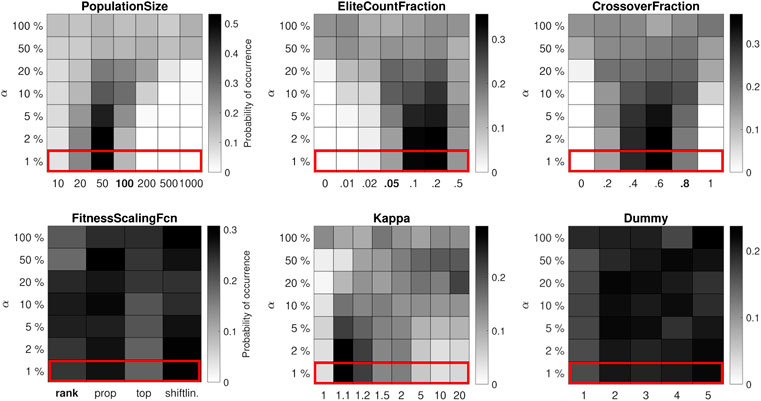
FIGURE 1. Distribution of control parameter values for the 10-bar truss test problem, where each run of the algorithm has a relatively low budget of 10⁴ function evaluations. The performance of the GA is significantly affected by the control parameter values.

The results for the low-budget case (10⁴ function evaluations) are shown in Figure 1. The GA finds the best known solution to the problem in 2% of runs, making the results for the top 1 and 2% identical. The best-performing value for the PopulationSize is 50, which corresponds to a maximum of 200 generations. The best-performing EliteCountFraction (the fraction of good designs that is maintained between generations) is somewhere in the range of 0.1–0.2, and the best-performing value for the CrossoverFraction is 0.6. All probability distributions in the top 1% appear to be unimodal, with the mode of the distribution for the PopulationSize being the most distinct. The distribution of values for the penalty parameter has a sharp peak near $\kappa =1.1$, which is in line with findings by e.g. Richardson et al. (1989) who argue that penalties that are too low unjustly promote infeasible designs, whereas penalties that are too high discard useful information from designs that are only slightly infeasible. No significant conclusions can be drawn for FitnessScalingFcn, although the second and fourth options seem to perform slightly better than the others, or for the Dummy parameter, which is to expected as it has no effect on the GA. The variability still present here shows the extent to which the algorithm has converged, illustrating the difference between control parameters that do have an effect and those that do not.

For the medium-budget case (10⁵ function evaluations) in Figure 2, the best-performing value for the PopulationSize is 500, which again corresponds to a maximum of 200 generations. The mode of the other parameter value distributions is similar to the low-budget case, but the variance is generally larger: the best-performing values are the same, but the GA is less sensitive to the control parameters. The same goes for the high-budget case (10⁶ function evaluations) in Figure 3, where it is better to use a PopulationSize of 1,000 (and maybe larger), which still allows the algorithm to run for up to 1,000 generations. Unsurprisingly, a clear trade-off is observed between the size of the population on the one hand and the maximum number of generations on the other. Furthermore, the results confirm that the impact of the control parameters is largest when the computation budget is small and less pronounced otherwise, in line with classic (theoretical) proofs that many metaheuristic algorithms are guaranteed to find the global optimum if one lets them run indefinitely (Rudolph, 1994).

FIGURE 2

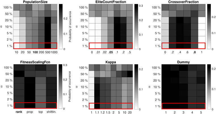
FIGURE 2. Distribution of control parameter values for the 10-bar truss test problem, where each run of the algorithm has a medium budget of 10⁵ function evaluations. The performance of the GA is less affected by the control parameter values.

FIGURE 3

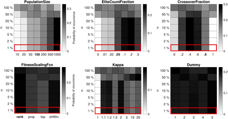
FIGURE 3. Distribution of control parameter values for the 10-bar truss test problem, where each run of the algorithm has a high budget of 10⁶ function evaluations. Apart from a few extremes, the effect of the control parameter values is less important.

It should be noted that parameter dependencies cannot be read directly from the figures. However, the relevant dependencies (those that give rise to good performance) are implicitly included in the well-performing subset of results from the Monte Carlo simulation. Limiting inferences to this subset prevents unimportant parameter interactions from obscuring the conclusions.

The performance threshold values $m_k$ in each stage k of the low-, medium- and high-budget case are shown in Table 2. The best design obtained during the experiment has an objective function value of 5490.74 lb, equaling the best known solution to this problem in the literature. For the low-budget case, the GA will achieve this objective function value in 2% of runs, when parameter values are randomly drawn from f. For the medium-budget case, the GA will achieve this value in 10% of runs, and for the high-budget case even in 20% of runs, showing that the GA is quite robust for its control parameters (for this problem) if the computational budget is large enough. The results in Table 2 can be used to compare the GA with other algorithms once a set of plausible parameter values is defined, which of course is still somewhat subjective.

TABLE 2

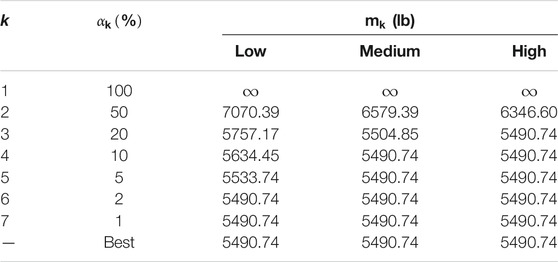
TABLE 2. Performance threshold values in stage k for a low, medium and high computational budget.

4.2 Comparison Between Multiple Test Problems

The second experiment compares the best-performing control parameter values for all seven test problems and aims to determine whether any general conclusions can be drawn. In all test problems, the GA is limited to 10⁵ function evaluations per run. The results for the 10-bar truss problem have already been presented in Figure 2. The results for the 25-, 52-, 47-, and 200-bar truss problems are shown in Figures 4–7, in order of increasing number of design variables. The Dummy parameter is omitted. At the end of the section, the results for the complete set of test problems are analyzed for trends regarding well-performing parameter values.

FIGURE 4

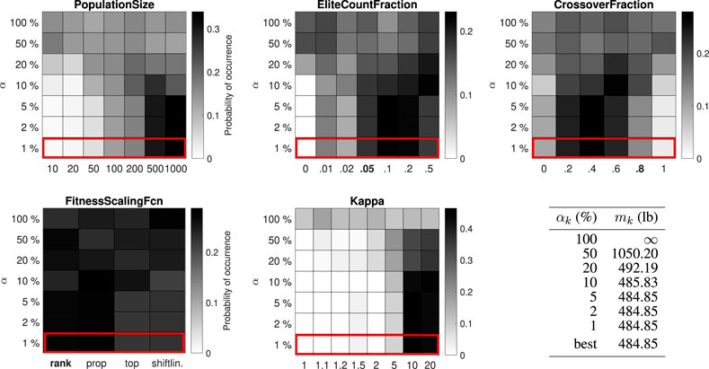
FIGURE 4. Distribution of control parameter values for the 25-bar truss test problem (8 design variables). The GA is limited to 10⁵ function evaluations within a single run. The default value for the PopulationSize is 80, which is not present among the options.

FIGURE 5

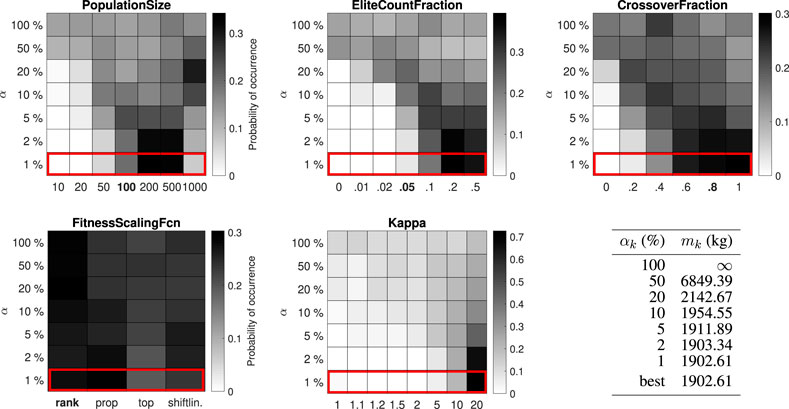
FIGURE 5. Distribution of control parameter values for the 52-bar truss test problem (12 design variables).

FIGURE 6

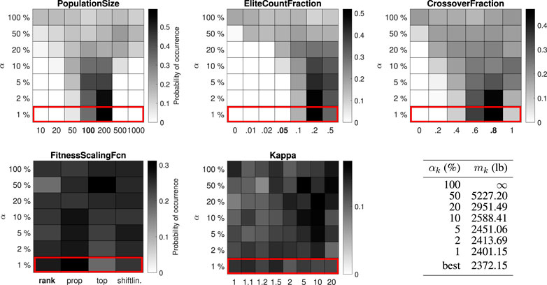
FIGURE 6. Distribution of control parameter values for the 47-bar truss test problem (27 design variables).

FIGURE 7

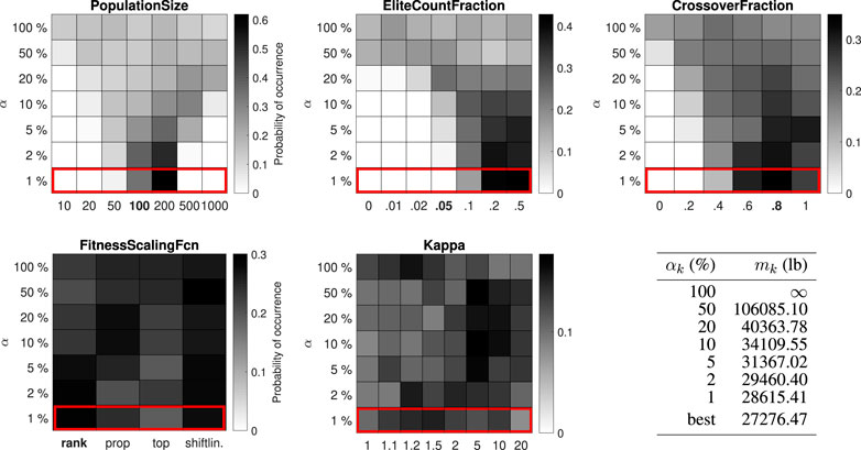
FIGURE 7. Distribution of control parameter values for the 200-bar truss test problem (29 design variables).

The best-performing value for the PopulationSize varies between 200 and 1,000 for the different test problems. The best-performing value for the EliteCountFraction ranges from 0.1 to 0.5. The best-performing value for the CrossoverFraction ranges from 0.4 to 1. The results for the FitnessScalingFcn are inconclusive, although the third option (“fitscalingtop”) consistently performs worse. For the small-scale problems (25-bar truss and 52-bar truss) the performance is higher with high values for the penalty parameter κ, while for the large-scale problems (47-bar truss and 200-bar truss) no significant difference can be observed.

For the 25-bar truss and 52-bar truss problems, the best objective function value from the simulation (484.85 lb and 1902.61 kg) is equal to the best solution in the literature. For the 47-bar truss and 200-bar truss problems, the best objective function value from the simulation (2372.15 and 27276.47 lb) is, to the authors’ best knowledge, slightly better than the best known solution in the literature (2376.02 and 27282.57 lb, associated design variables are given in Supplementary Appendix SB). With enhanced control parameter values, the GA has succeeded in improving the best known solution to the last two (well-studied) test problems, providing the community with new benchmark results while demonstrating the strength of the proposed method.

The number of sample runs and objective function evaluations performed in this experiment are listed in Table 3. They are of the same order of magnitude as reported for existing parameter tuning methods (Montero et al., 2014), depending on the accuracy of the estimates and the computational budget of the algorithm. Nevertheless, the computing power required to make the assessment is high. Investing such effort may be particularly relevant for optimizing parameters for a set of similar problems, for finding new benchmark results (optimal solutions) for the test problems, or for looking for general trends in important parameters and well-performing parameter values for specific types of optimization problems, such as discrete truss sizing optimization problems. The latter is investigated in the next paragraph.

TABLE 3

TABLE 3. Summary of the computations for the 4 test problems, expressed as the number of sample runs and number of objective function evaluations (throughout the simulation).

Figure 8 summarizes the top 1% parameter value distributions of all problems in the test set, shown in order of increasing problem size (number of discrete solutions in the design space). Some trends do seem to emerge. The best-performing value for the PopulationSize decreases with the problem size, while the function evaluation limit remains constant, corresponding to an increasing number of allowable generations. The best-performing values for the EliteCountFraction and the CrossoverFraction generally increase with the problem size, although often multiple options perform similarly (e.g. CrossoverFraction equal to 0.6, 0.8 or 1 for the 52-bar truss problem or EliteCountFraction equal to 0.2 or 0.5 for the 200-bar truss problem). The results for FitnessScalingFcn are not statistically significant, but the second option (“fitscalingprop”) consistently performs well and the third option (“fitscalingtop”) always performs poorly. Good values for κ cannot be predicted based on the size of the optimization problem alone, although its effect is less important when the problem size is large. Robust parameter values (i.e. values that perform well for all test problems) are 200 for the PopulationSize, 0.2 for the EliteCountFraction and 0.6 or 0.8 for the CrossoverFraction. Robust values for FitnessScalingFcn are “fitscalingrank” (the default value) and “fitscalingprop.” Finally, a high value for κ is always a safe choice.

FIGURE 8

FIGURE 8. Comparison of the top 1% parameter value distributions for all optimization problems in the test set. The results are ordered according to the number of discrete solutions in the design space (the problem size).

The conclusions for the second experiment are as follows. For all test problems, the impact of the PopulationSize, the EliteCountFraction and the CrossoverFraction is significant, and the mode of the corresponding parameter value distribution becomes clearer as the problem size increases (with a fixed computational budget). Similar to the first experiment, the impact of the control parameters is larger when the computational budget is small. The best-performing value for the EliteCountFraction is consistently higher than the default value in matlab. The best-performing value for the CrossoverFraction varies, and seems to be proportional to the problem size. The best-performing value for the PopulationSize depends on the problem size and on the computational budget of the algorithm. The best-performing control parameter values found by the proposed method do not always match the default values in matlab.

4.3 Default vs. Optimized Control Parameter Values

The best-performing control parameter values found in the previous subsection are generally not the default values in matlab. Hence, the performance of the GA with default parameter values (listed in Table 4) is compared to the performance of the algorithm with optimized control parameter values (well-performing values from the previous subsection, listed in Table 5).

TABLE 4

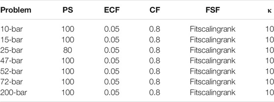
TABLE 4. Default values for the control parameters. Their names are abbreviated as follows: PopulationSize (PS), EliteCountFraction (ECF), CrossoverFraction (CF), FitnessScalingFcn (FSF), and penalty parameter κ.

TABLE 5

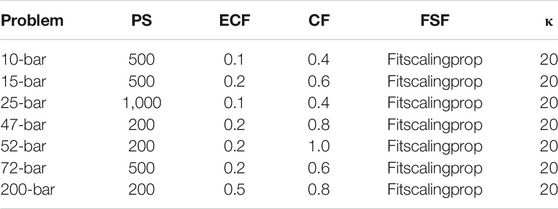
TABLE 5. Optimized values for the control parameters.

The results of the comparison are summarized in Figure 9, using (custom) box plots. Each box plot represents 100 independent runs of the GA, with random starting points and a computational budget of 10⁵ function evaluations. Infeasible solutions are given an objective function value of infinity. If (part of) a box plot is cut off at the top of the figure, it means that the corresponding objective function value goes to infinity.

FIGURE 9

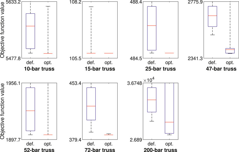
FIGURE 9. Summary of results of the GA when applied to the truss test problems, with default (def.) and optimized (opt.) control parameter values. The system (bottom whisker, box bottom, middle, top, top whisker) denotes the (minimum, 10-th percentile, median, 90-th percentile, maximum) objective function value in 100 independent runs of the GA.

The figure shows that the performance of the GA with optimized control parameter values is better than the performance with default values in almost all possible areas. For the 10-, 15-, 25- 52-, and 72-bar truss problems, the GA matches the best known solution in the literate in at least 90% of runs, and even in 100% of runs for the 15- and 25-bar truss problems, performing significantly better than with default control parameter values. For the 47-bar truss problem, the best result in the simulation (2377.5 lb) is slightly less good than the best result in the literature (2372.2 lb in this article, 2376.0 lb otherwise), but again the performance of the algorithm is considerably better than with default parameter values. For the 200-bar truss, the extremes of performance are amplified: the minimum, 10-th percentile and median objective function values are a lot better with optimized parameter values, although the algorithm more often converges to an infeasible design. With default control parameter values, at least one infeasible design is present among the results for 6 out of 7 test problems, compared to 3 out of 7 test problems in the case of optimized control parameter values.

5 Conclusions

A method has been developed to assess the performance of a metaheuristic algorithm in relation to the values of the control parameters. It is based on Monte Carlo sampling of independent algorithm runs and uses importance sampling as a variance reduction technique. The method is demonstrated using the genetic algorithm (GA) built into matlab for seven representative discrete truss sizing optimization problems that are commonly used in structural optimization literature. The method successfully captured the sensitivity of the GA with respect to the control parameters, identifying relevant parameters whose values need careful tuning as well as parameters that have little impact for the problems at hand. For the important control parameters, well-performing values are identified that consistently outperform the default matlab values for the benchmark problems considered.

The results in this study indicate that the impact of the control parameters is largest when the limit on the number of function evaluations is low. When the limit on the number of function evaluations is high, the algorithm becomes more robust to the values of its control parameters, affirming that longer computing times can (partially) compensate for poor parameter value choices.

The method described in this study can be used in a variety of ways. Information on the sensitivity of an optimization algorithm with respect to its control parameters can help developers to focus on the relevant part of their algorithm. In addition, the method can be used to select appropriate default values for the control parameters based on a representative set of test problems. The performance percentiles resulting from the simulation can be used to compare the algorithm with other metaheuristic algorithms. Finally, the Monte Carlo simulation may provide the academic community with new benchmark results, as illustrated by the improvements over the best designs reported so far in the literature for the 47-bar truss and the 200-bar truss test problems (found in Section 4 of this article).

Using the method to find good control parameter values is computationally expensive, as it requires several optimization runs to be performed. Therefore, it may be worthwhile to look for general guidelines regarding control parameter values that perform well. The results of all seven test problems have been compared to look for dependencies between well-performing parameter values and the number of discrete solutions in the design space. Robust parameter values (values that perform reasonably well for all problems in the test set) have been identified. For the test problems considered, it is found that the best-performing value for the PopulationSize of the GA heavily depends on the size of the optimization problem, and on the maximum number of function evaluations in a single run of the algorithm. Furthermore, it is found that the best-performing value for the EliteCountFraction is consistently higher than the default setting, and that the best-performing value for the CrossoverFraction is roughly proportional to the size of the design space.

Data Availability Statement

The source code of the example problems presented in the study are included in the article/Supplementary Material, further inquiries can be directed to the corresponding author.

Author Contributions

WD: methodology, software, analysis, writing, and editing. GL: conceptualization, methodology, supervision, reviewing. MS: conceptualization, methodology, supervision, reviewing.

Funding

This work has been performed in the frame of project C24/15/012 funded by the Industrial Research Fund of KU Leuven. The financial support is gratefully acknowledged.

Conflict of Interest:

The authors declare that the research was conducted in the absence of any commercial or financial relationships that could be construed as a potential conflict of interest.

Supplementary Material

The Supplementary Material for this article can be found online at: https://www.frontiersin.org/articles/10.3389/fbuil.2021.618851/full#supplementary-material.

Footnotes

¹In a computer implementation, the random behavior of the algorithm will be determined by the seed that initializes the pseudorandom number generator. In this case, $H\left(\theta \right)$ is the function that maps each elementary event θ to a specific seed number h. Depending on the software, the number of possibilities for the random seed can be finite or infinite. Throughout this study, we assume that the number of possible seeds is either finite or countably infinite, in which case $H\left(\theta \right)$ is a discrete random variable. The case where $H\left(\theta \right)$ is continuous is similar, but it requires integrals instead of sums.

²The current methodology is based on discrete random variables. The use of continuous variables in combination with kernel density estimation may be interesting for further research, but it is beyond the scope of this article.

³The EliteCountFraction is used to control the number of “elite” individuals in the GA (the value of EliteCount), which is computed as EliteCountFraction × PopulationSize, rounded to the nearest integer smaller than PopulationSize. The matlab default value for the EliteCount is 0.05 × PopulationSize for continuous problems and 0.05 × default PopulationSize for discrete problems. However, in this paper, the EliteCount is expressed as a fraction of the actual PopulationSize, indicating 0.05 as the default EliteCountFraction value.

References

Adenso-Díaz, B., and Laguna, M. (2006). Fine-tuning of algorithms using fractional experimental designs and local search. Operations Res. 54, 99–114. doi:10.1287/opre.1050.0243

CrossRef Full Text | Google Scholar

Ansótegui, C., Sellmann, M., and Tierney, K. (2009). “A gender-based genetic algorithm for the automatic configuration of algorithms,” in International conference on principles and practice of constraint programming, Lisbon, Portugal, September, 2009 (Springer), 142–157.

Google Scholar

Audet, C., and Orban, D. (2004). Finding optimal algorithmic parameters using a mesh adaptive direct search. Cahiers du GERAD G-2004-xx, 41.

Google Scholar

Bäck, T., and Schwefel, H.-P. (1993). An overview of evolutionary algorithms for parameter optimization. Evol. Comput. 1, 1–23. doi:10.1162/evco.1993.1.1.1

CrossRef Full Text | Google Scholar

Balaprakash, P., Birattari, M., and Stützle, T. (2007). “Improvement strategies for the F-Race algorithm: sampling design and iterative refinement,” in International workshop on hybrid metaheuristics, Dortmund, Germany, October, 2007 (Springer), 108–122.

Google Scholar

Bartz-Beielstein, T. (2006). Experimental research in evolutionary computation. Berlin, Germany: Springer.

Bartz-Beielstein, T., Lasarczyk, C., and Preuß, M. (2005). “Sequential parameter optimization,” in IEEE congress on evolutionary computation. Edinburgh, United Kingdom, September, 2005 (IEEE), 1, 773–780.

Google Scholar

Bartz-Beielstein, T., Parsopoulos, K. E., and Vrahatis, M. N. (2004). Design and analysis of optimization algorithms using computational statistics. Appl. Num. Anal. Comp. Math. 1, 413–433. doi:10.1002/anac.200410007

CrossRef Full Text | Google Scholar

Beale, E. (1962). Some use of computers in operational research. Ind. Organ. 31, 27–28.

Google Scholar

Birattari, M., Stützle, T., Paquete, L., and Varrentrapp, K. (2002). “A racing algorithm for configuring metaheuristics,” in Proceedings of the 4th annual conference on genetic and evolutionary computation, New York, United States (New York, NY: Morgan Kaufmann Publishers Inc.), 11–18.

Google Scholar

Camp, C. V., and Bichon, B. J. (2004). Design of space trusses using ant colony optimization. J. Struct. Eng. 130, 741–751. doi:10.1061/(asce)0733-9445(2004)130:5(741)

CrossRef Full Text | Google Scholar

Castillo-Valdivieso, P., Merelo, J., Prieto, A., Rojas, I., and Romero, G. (2002). Statistical analysis of the parameters of a neuro-genetic algorithm. IEEE Trans. Neural Netw. 13, 1374–1394. doi:10.1109/TNN.2002.804281

PubMed Abstract | CrossRef Full Text | Google Scholar

Charalampakis, A., and Tsiatas, G. (2019). Critical evaluation of metaheuristic algorithms for weight minimization of truss structures. Front. Built Environ. 5, 113. doi:10.3389/fbuil.2019.00113

CrossRef Full Text | Google Scholar

Chiarandini, L., Preuss, M., Paquete, L., and Ridge, E. (2007). Experiments on metaheuristics: methodological overview and open issues. Technical report. Copenhagen (Denmark): Danish Mathematical Society.

Google Scholar

Choquet, D., L’Ecuyer, P., and Léger, C. (1999). Bootstrap confidence intervals for ratios of expectations. ACM Trans. Model. Comput. Simul. 9, 326–348. doi:10.1145/352222.352224

CrossRef Full Text | Google Scholar

Cornuet, J.-M., Marin, J.-M., Mira, A., and Robert, C. P. (2012). Adaptive multiple importance sampling. Scand. J. Stat. 39, 798–812. doi:10.1111/j.1467-9469.2011.00756.x

CrossRef Full Text | Google Scholar

Coy, S. P., Golden, B., Runger, G., and Wasil, E. (2001). Using experimental design to find effective parameter settings for heuristics. J. Heuristics 7, 77–97. doi:10.1023/a:1026569813391

CrossRef Full Text | Google Scholar

Czarn, A., MacNish, C., Vijayan, K., Turlach, B., and Gupta, R. (2004). Statistical exploratory analysis of genetic algorithms. IEEE Trans. Evol. Computat. 8, 405–421. doi:10.1109/tevc.2004.831262

CrossRef Full Text | Google Scholar

De Jong, K. (1975). Analysis of the behavior of a class of genetic adaptive systems. PhD thesis. Ann Arbor (MI): University of Michigan, Computer and Communication Sciences Department.

Google Scholar

Degertekin, S. O., Lamberti, L., and Ugur, I. B. (2019). Discrete sizing/layout/topology optimization of truss structures with an advanced Jaya algorithm. Appl. Soft Comput. 79, 363–390. doi:10.1016/j.asoc.2019.03.058

CrossRef Full Text | Google Scholar

Dillen, W., Lombaert, G., Voeten, N., and Schevenels, M. (2018). “Performance assessment of metaheuristic algorithms for structural optimization taking into account the influence of control parameters,” in Proceedings of the 6th international conference on engineering optimization (Lisbon, Portugal: Springer), 93–101.

CrossRef Full Text | Google Scholar

Dobslaw, F. (2010). “A parameter tuning framework for metaheuristics based on design of experiments and artificial neural networks,” in International Conference on computer Mathematics and natural computing (WASET), Rome, Italy, April, 2010.

Google Scholar

Dolan, E. D., and Moré, J. J. (2002). Benchmarking optimization software with performance profiles. Math. Programming 91, 201–213. doi:10.1007/s101070100263

CrossRef Full Text | Google Scholar

Eiben, A. E., and Smit, S. K. (2011). Parameter tuning for configuring and analyzing evolutionary algorithms. Swarm Evol. Comput. 1, 19–31. doi:10.1016/j.swevo.2011.02.001

CrossRef Full Text | Google Scholar

Falkner, S., Klein, A., and Hutter, F. (2018). “Bohb: robust and efficient hyperparameter optimization at scale,” in Proceedings of the 35th international conference on machine learning (ICML), Stockholm, Sweden, July, 2018.

Google Scholar

Georgioudakis, M., and Plevris, V. (2020). A comparative study of differential evolution variants in constrained structural optimization. Front. Built Environ. 6, 102. doi:10.3389/fbuil.2020.00102

CrossRef Full Text | Google Scholar

Gholizadeh, S., Danesh, M., and Gheyratmand, C. (2020). A new Newton metaheuristic algorithm for discrete performance-based design optimization of steel moment frames. Comput. Structures 234, 106250. doi:10.1016/j.compstruc.2020.106250

CrossRef Full Text | Google Scholar

Gomes, W. J. S., Beck, A. T., Lopez, R. H., and Miguel, L. F. F. (2018). A probabilistic metric for comparing metaheuristic optimization algorithms. Struct. Saf. 70, 59–70. doi:10.1016/j.strusafe.2017.10.006

CrossRef Full Text | Google Scholar

Grefenstette, J. (1986). Optimization of control parameters for genetic algorithms. IEEE Trans. Syst. Man. Cybern. 16, 122–128. doi:10.1109/tsmc.1986.289288

CrossRef Full Text | Google Scholar

Haftka, R. T. (2016). Requirements for papers focusing on new or improved global optimization algorithms. Struct. Multidisc Optim. 54, 1. doi:10.1007/s00158-016-1491-5

CrossRef Full Text | Google Scholar

Hammersley, J., and Handscomb, D. (1964). Monte Carlo methods. Berlin, Germany: Springer Science and Business Media.

CrossRef Full Text

Hasançebi, O. (2008). Adaptive evolution strategies in structural optimization: enhancing their computational performance with applications to large-scale structures. Comput. Structures 86, 119–132. doi:10.1016/j.compstruc.2007.05.012

CrossRef Full Text | Google Scholar

Hasançebi, O., Erdal, F., and Saka, M. (2009). Adaptive harmony search method for structural optimization. J. Struct. Eng. 136, 419–431. doi:10.1061/(ASCE)ST.1943-541X.0000128

CrossRef Full Text | Google Scholar

Ho-Huu, V., Nguyen-Thoi, T., Vo-Duy, T., and Nguyen-Trang, T. (2016). An adaptive elitist differential evolution for optimization of truss structures with discrete design variables. Comput. Structures 165, 59–75. doi:10.1016/j.compstruc.2015.11.014

CrossRef Full Text | Google Scholar

Hooker, J. N. (1995). Testing heuristics: we have it all wrong. J. Heuristics 1, 33–42. doi:10.1007/bf02430364

CrossRef Full Text | Google Scholar

Hutter, F., Hoos, H. H., Leyton-Brown, K., and Stuetzle, T. (2009b). ParamILS: an automatic algorithm configuration framework. JAIR 36, 267–306. doi:10.1613/jair.2861

CrossRef Full Text | Google Scholar

Hutter, F., Hoos, H., Leyton-Brown, K., and Murphy, K. (2009a). “An experimental investigation of model-based parameter optimisation: SPO and beyond,” in Proceedings of the 11th Annual conference on Genetic and evolutionary computation, Montréal, Canada, July, 2009 (ACM), 271–278.

Google Scholar

Hutter, F., Hoos, H., Leyton-Brown, K., and Murphy, K. (2010). “Time-bounded sequential parameter optimization,” in International conference on learning and intelligent optimization, Kalamata, Greece, June, 2010 (Springer), 281–298.

CrossRef Full Text | Google Scholar

Hutter, F., Hoos, H., and Leyton-Brown, K. (2011). “Sequential model-based optimization for general algorithm configuration.” in International conference on learning and intelligent optimization, Rome, Italy, January, 2011 (Springer), 507–523.

CrossRef Full Text | Google Scholar

Jaynes, E. (2003). Probability theory: the logic of science. Cambridge, United Kingdom: Cambridge University Press.

Karafotias, G., Hoogendoorn, M., and Eiben, A. E. (2015). Parameter control in evolutionary algorithms: trends and challenges. IEEE Trans. Evol. Computat. 19, 167–187. doi:10.1109/tevc.2014.2308294

CrossRef Full Text | Google Scholar

Kaveh, A., and Farhoudi, N. (2011). A unified approach to parameter selection in meta-heuristic algorithms for layout optimization. J. Constructional Steel Res. 67, 1453–1462. doi:10.1016/j.jcsr.2011.03.019

CrossRef Full Text | Google Scholar

Kolmogorov, A. (1956). Foundations of the theory of probability. New York, NY: Chelsea Publishing Company.

Le Riche, R., and Haftka, R. T. (2012). On global optimization articles in SMO. Struct. Multidisc Optim. 46, 627–629. doi:10.1007/s00158-012-0785-5

CrossRef Full Text | Google Scholar

Lee, K. S., Geem, Z. W., Lee, S.-h., and Bae, K.-W. (2005). The harmony search heuristic algorithm for discrete structural optimization. Eng. Optimization 37, 663–684. doi:10.1080/03052150500211895

CrossRef Full Text | Google Scholar

Lepage, G. (1978). A new algorithm for adaptive multidimensional integration. J. Comput. Phys. 27, 192–203.

Google Scholar

Li, L., Jamieson, K., DeSalvo, G., Rostamizadeh, A., and Talwalkar, A. (2017). Hyperband: a novel bandit-based approach to hyperparameter optimization. J. Machine Learn. Res. 18, 6765–6816.

Google Scholar

López-Ibáñez, M., Dubois-Lacoste, J., Pérez Cáceres, L., Birattari, M., and Stützle, T. (2016). The irace package: iterated racing for automatic algorithm configuration. Operations Res. Perspect. 3, 43–58. doi:10.1016/j.orp.2016.09.002

CrossRef Full Text | Google Scholar

McGill, R., Tukey, J. W., and Larsen, W. A. (1978). Variations of box plots. The Am. Statistician 32, 12–16. doi:10.2307/2683468

CrossRef Full Text | Google Scholar

Montero, E., Riff, M.-C., and Neveu, B. (2014). A beginner’s guide to tuning methods. Appl. Soft Comput. 17, 39–51. doi:10.1016/j.asoc.2013.12.017

CrossRef Full Text | Google Scholar

Moré, J. J., and Wild, S. M. (2009). Benchmarking derivative-free optimization algorithms. SIAM J. Optim. 20, 172–191. doi:10.1137/080724083

CrossRef Full Text | Google Scholar

Myers, R., and Hancock, E. (2001). Empirical modelling of genetic algorithms. Evol. Comput. 9, 461–493. doi:10.1162/10636560152642878

PubMed Abstract | CrossRef Full Text | Google Scholar

Nannen, V., and Eiben, A. (2007). Relevance estimation and value calibration of evolutionary algorithm parameters. IJCAI 7, 975–980. doi:10.1109/CEC.2007.4424460

Google Scholar

Nickabadi, A., Ebadzadeh, M. M., and Safabakhsh, R. (2011). A novel particle swarm optimization algorithm with adaptive inertia weight. Appl. Soft Comput. 11, 3658–3670. doi:10.1016/j.asoc.2011.01.037

CrossRef Full Text | Google Scholar

Ogliore, R. C., Huss, G. R., and Nagashima, K. (2011). Ratio estimation in SIMS analysis. Nucl. Instrum. Methods Phys. Res., B 269, 1910–1918. doi:10.1016/j.nimb.2011.04.120

CrossRef Full Text | Google Scholar

Owen, A., and Zhou, Y. (2000). Safe and effective importance sampling. J. Am. Stat. Assoc. 95, 135–143. doi:10.1080/01621459.2000.10473909

CrossRef Full Text | Google Scholar

Owen, A., and Zhou, Y. (1999). Adaptive importance sampling by mixtures of products of beta distributions. Technical report. Stanford (CA): Stanford University.

Google Scholar

Rajeev, S., and Krishnamoorthy, C. S. (1992). Discrete optimization of structures using genetic algorithms. J. Struct. Eng. 118, 1233–1250. doi:10.1061/(asce)0733-9445(1992)118:5(1233)

CrossRef Full Text | Google Scholar

Rardin, R. L., and Uzsoy, R. (2001). Experimental evaluation of heuristic optimization algorithms: a tutorial. J. Heuristics 7, 261–304. doi:10.1023/a:1011319115230

CrossRef Full Text | Google Scholar

Rechenberg, I. (1973). Evolution strategy: optimization of technical systems by means of biological evolution. Frommann-Holzboog, Stuttgart 104, 15–16.

Google Scholar

Richardson, J., Palmer, M., Liepins, G., and Hilliard, M. (1989). “Some guidelines for genetic algorithms with penalty functions, in Proceedings of the 3rd international conference on genetic algorithms, Fairfax, VA, June, 1989 (Morgan Kaufmann Publishers Inc.), 191–197.

Google Scholar

Rudolph, G. (1994). Convergence analysis of canonical genetic algorithms. IEEE Trans. Neural Netw. 5, 96–101. doi:10.1109/72.265964

PubMed Abstract | CrossRef Full Text | Google Scholar

Sacks, J., Welch, W. J., Mitchell, T. J., and Wynn, H. P. (1989). Design and analysis of computer experiments. Statist. Sci., 4, 409–423. doi:10.1214/ss/1177012413

CrossRef Full Text | Google Scholar

Stuart, A., and Ord, J. (1994). Kendall’s advanced theory of statistics. 6 Edn. London, United Kingdom: Edward Arnold, 1.

Wolpert, D. H., and Macready, W. G. (1997). No free lunch theorems for optimization. IEEE Trans. Evol. Computat. 1, 67–82. doi:10.1109/4235.585893

CrossRef Full Text | Google Scholar

Xu, J., Chiu, S. Y., and Glover, F. (1998). Fine-tuning a tabu search algorithm with statistical tests. Int. Trans. Oper. Res. 5, 233–244. doi:10.1111/j.1475-3995.1998.tb00117.x

CrossRef Full Text | Google Scholar

Yuan, B., and Gallagher, M. (2007). “Combining meta-EAs and racing for difficult EA parameter tuning tasks,” in Parameter setting in evolutionary algorithms (Berlin, Germany: Springer), 121–142.

Google Scholar