Mobile Monitoring of Air Pollution Reveals Spatial and Temporal Variation in an Urban Landscape

Introduction

Air pollution is a major environmental threat for urban populations, affecting the health of 9 out of 10 urban residents (World Health Organization, 2018). Within urban environments, locally high concentrations of air pollutants are common (Strosnider et al., 2017). As populations continue to migrate to urban areas (United Nations, 2019), air pollution will prove a persistent and growing threat to urban populations; this threat is pronounced for subsets of the population who are of lower socioeconomic status or are physiologically vulnerable to air pollutants due to age or pre-existing conditions, as these groups are disproportionately impacted by the negative health impacts of air pollution (Perlin et al., 1999; Zhou et al., 2011; Gray et al., 2013). In order to attenuate negative health impacts of air pollution in the future, it is imperative that we accurately assess the spatiotemporal distribution of air pollution in urban environments. Comprehensive air pollution monitoring is crucial to understanding where, and how, to focus efforts to attenuate air pollution and its associated health risks in cities equitably.

PM consists of heterogeneous mixtures of organic (Tsapakis et al., 2002) and inorganic components (Kelly and Fussell, 2012) that vary in size, shape, composition, and origin within the urban environment (City of Philadelphia, 2019; Shakya et al., 2019). Coarse size fractions (PM_2.5–PM₁₀) of PM largely originate from crustal sources, whereas fine PM (PM_0.1–PM_2.5) derive mainly from industrial emissions, non-renewable power generation, and vehicle exhausts (United States Environmental Protection Agency, 2015). BC is a major component of PM that results from the incomplete combustion of fossil fuels and other organic matter. As such, the presence of BC is often used as an indicator of urban traffic pollution (Targino et al., 2016). Quantifying the abundance and distribution of various PM sizes in urban environments is of particular interest to public health (Dominici et al., 2006), as prolonged exposure to PM is associated with increased rates of mortality (Dockery et al., 1993); smaller particles, especially those within finer size fractions, can easily deposit in the lungs (Miller et al., 1979), leading to a number of negative health outcomes including reduced lung function (Shakya et al., 2016), asthma (Rabinovitch et al., 2006), cardiovascular and respiratory disease (Paul et al., 2019), and pathogen exposure (Cao et al., 2014; Stewart et al., 2021).

Many studies have investigated urban air quality, but such studies typically rely on a small number of stationary points of measurement (Vallius et al., 2005; Zhang and Cao, 2015) and interpolation (Burke et al., 2001; Zhang et al., 2013) to characterize air pollution across an entire city. While these methods are effective at capturing temporal trends in local pollutant concentrations, they are less able to capture fine-scale spatial variation in air pollution throughout urban environments. This is crucial in urban areas, where emissions sources are not uniformly distributed and pollutant dispersal patterns change over short distances due to differences in vegetation (Brantley et al., 2014; Gromke & Ruck, 2012; Salmond et al., 2013; Xing & Brimblecombe 2019) and urban structure (Abhijith and Gokhale, 2015; Gallagher et al., 2015; Hagler et al., 2012). In recent years, mobile monitoring has emerged as a novel method with which to study the spatial and temporal distribution of air pollutants (Van Poppel et al., 2013; Deville Cavellin et al., 2016; Targino et al., 2016; Apte et al., 2017; Shakya et al., 2019; Sm et al., 2019; deSouza et al., 2020). As mobile monitoring methods are capable of collecting data at finer spatial scales than is feasible with stationary monitoring (Van den Bossche et al., 2015; Shakya et al., 2019), mobile monitoring is capable of providing more accurate and meaningful information about air quality in Philadelphia and can identify areas where pollutants with detrimental health impacts pose the greatest risk to human health.

In this study, we employ vehicular mobile monitoring of PM across 24 different size fractions between 0.25–10 μm and BC throughout the urban landscape of Philadelphia, Pennsylvania during the summer of 2019. Mobile monitoring allows us to observe the spatiotemporal distribution of air pollutants and discern patterns in variation at a fine spatial scale (Gozzi et al., 2016), and in doing so, identify times and locations in an urban environment such as Philadelphia where high concentrations of air pollutants are prevalent. Using Getis-Ord Gi* hot spot analysis, we identify where and when hotspots of air pollution occur to determine where statistically significant high air pollutant concentrations appear consistently. With a more fine-scale, holistic assessment of urban air pollution, cities can determine where air quality improvements are most needed, and better develop strategies intended to reduce ambient air pollution through future urban planning and development.

Methods

Site Description

Philadelphia, Pennsylvania is the sixth-largest city in the United States and the largest city in the state of Pennsylvania, with an estimated population of 1,584,138 in 2018. With an area of 143 mi² (370 km²), Philadelphia is dominated by a dense urban center surrounded by predominantly low-rise residential and commercial districts, city parks, and industrial sectors. The city’s eastern border is defined by the Delaware River, which flows southward to the Delaware Bay and Atlantic Ocean; the city’s other major river, the Schuylkill River, flows southward to the Delaware through the western neighborhoods of Philadelphia. The southern and eastern parts of the city house heavy industry along both riverbanks (Lower Southwest, Lower South, and River Wards Planning Districts), while large park areas are found in the western and northern areas of the city (Lower Northwest, Upper Northwest, and Central Northeast Planning Districts) (Figure 1).

FIGURE 1

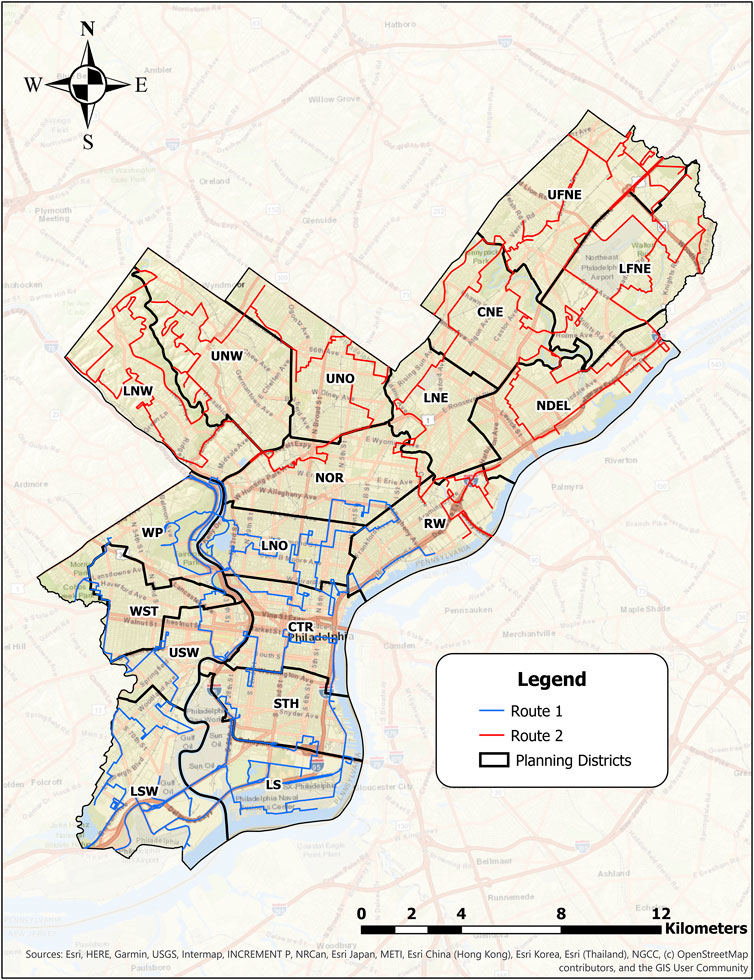
FIGURE 1. Map of study area, including routes traveled for mobile air pollution monitoring and Philadelphia planning districts. Abbreviations on the map denote each planning district in Philadelphia.

Sampling Description

A van, equipped with two global positioning system (GPS) units (Trimble Juno 3 B fitted with Trimble R1 GNSS receivers) and instrumentation measuring PM₁, PM_2.5, and PM₁₀ concentrations along with mass values for 24 different size fractions (Grimm Portable Laser Aerosol Spectrometer, Model 11-C) and BC (MicroAeth MA200), was driven along the two predetermined routes (∼150 miles/∼241.4 km each) in Philadelphia (Supplementary Table S1). The Grimm spectrometer was factory calibrated prior to the monitoring campaign. Air pollution instrumentation was placed inside a box attached to the roof of a van (∼1.5 m), and the inlets of the instrumentation were connected to an isokinetic sampling probe of diameter 1.5 mm. The instrumentation used is ideal for mobile monitoring studies (Hussein et al., 2008; Yu et al., 2016); in addition to being lightweight and battery-operated, the monitoring equipment provides data with high temporal resolution. To maintain continuous measurements in the face of satellite reception issues and equipment malfunction, the two GPS units were used simultaneously. Data was captured at different temporal resolutions; GPS data was recorded for every 1 s interval, while BC data was recorded every 5 s and PM data was recorded every 6 s.

The driving routes were developed using a stratified random selection of points representing different combinations of urban structure to provide a representative sample of Philadelphia. Additionally, selected points of interest, such as United States Environmental Protection Agency (U.S. EPA) Toxics Release Inventory (TRI) sites, EPA air pollution monitoring station sites, Philadelphia Water Department’s green infrastructure sites, and census tracts with high rates of asthma were included in route development. The optimized driving route, which passed through the selected sample points, was created using ESRI ArcGIS 10.7.1 Network Analyst, and the resulting 300 mile (482.8 km) route was then split into two near-equal length segments of approximately 150 miles each, with each segment being drivable in a single day (Figure 1). Occasional road closures in Philadelphia created slight variability in the routes traveled from day to day (Supplementary Figure S1).

Measurements were conducted over a period of 12 days between June 27 and July 29, 2019; sampling occurred on days where inclement weather (i.e. rain) did not pose a risk to the monitoring equipment. Measurement began between the hours of 6:00 AM and 7:00 AM on one of the two routes and continued until the entirety of the route was travelled; the sampling period on any given day ranged from about 8 to 10.5 h (Supplementary Table S2). The average daily speed of the vehicle ranged from 23.3–29.9 km/h (14.5–18.6 mph), estimated by dividing the length of the routes by the sampling times.

Data Processing/Analysis

Instrument reported air pollutant concentrations and GPS data were joined by time to create a database of geolocated air pollution data. For each day, the top and bottom 0.5% of air pollution measurements were removed to account for outliers in the dataset. Pollution data lacking geolocation information due to instrument error was not considered for spatial analysis in this paper. One day (July 15, 2019) is entirely excluded from spatial analysis as a result of GPS malfunction that resulted in a significant amount of missing geolocation data. Though emissions from nearby vehicles can influence instantaneous measurements of pollutant concentrations, we choose not to filter these out, as these can offer valuable insights regarding traffic density in Philadelphia, the impact of vehicles on ambient concentrations of pollutants at large, and the exposure of nearby pedestrians to high pollutant concentrations. Further, the quantity of data points obtained coupled with data aggregation ensures that average concentrations are accurately represented despite the potential for differences in local conditions from day-to-day (Van den Bossche et al., 2015).

Spatial analysis was conducted in ESRI ArcGIS Pro 2.4. Point datasets were projected into the Pennsylvania State Plane South projected coordinate system. Air pollution data was spatially joined to a systematic grid of 120 m² fishnet cells overlaid on Philadelphia, which has previously been used to generalize and characterize urban landscape and ecosystem function (Hamstead et al., 2016; Shakya et al., 2019; Stewart et al., 2021). All points falling within a given cell were averaged to determine the average concentration of pollutants in that 120 m² area. For each day of data collection, PM₁, PM_2.5, PM₁₀, and BC hotspots with statistical significance at a 95% confidence level were identified using the Hot Spot Analysis (Getis-Ord Gi*) tool. Hot spot analysis allows for the identification of statistically significant locations in a study area where features with high or low values cluster within the context of its neighborhood (Getis and Ord, 1992). Each point in the dataset is assigned a $G_i^{\ast }$ value, given by the following equation, where $w_{i,j}$ is the spatial weight between two observations, $x_i$ and $x_j$, $\overline{x}$ is the average of all observed values, and $n$ is the sample size (Getis and Ord, 1992):

$G_i^{\ast }=\frac{{{\displaystyle \sum }}_{j=1}^n{w}_{i,j}{x}_j-\overline{x}{{\displaystyle \sum }}_{j=1}^n{w}_{i,j}}{\sqrt{{{\displaystyle \sum }}_{j=1}^n{x}_j^2/n}-{\left(\overline{x}\right)}^2\ast \sqrt{\left[n{{\displaystyle \sum }}_{j=1}^n{w}_{\text{i},j}^2-{\left({{\displaystyle \sum }}_{j=1}^n{w}_{i,j}\right)}^2\right]/n-1}}$

The neighborhood threshold radius for all hot spot analyses was set at the minimum distance to ensure that for each day, observations for all pollutants measured had at least one other feature designated as a neighbor (615 m). The inverse distance squared conceptualization of spatial relationships was used for this analysis, which sees the influence (spatial weight) of an observation on its spatial neighbors decrease significantly with increasing distance. False discovery rate correction was applied to correct for false positives. To compare the locations of hotspots across the days of data collection, significant hotspots (p < 0.05) for each day were spatially joined with the fishnet grid. Hotspots within a given cell were averaged to determine the mean pollution concentration of the hotspots in each cell for each day.

Statistical analysis was conducted in R (3.6.1). Combination violin and boxplots were produced to show the range and distribution of air pollutants across all days. In this study, we collected a large amount of data (“big data”) based on counts, which leads to overdispersion of datapoints and zero-inflation (Aitchison and Ho, 1989) that are replicated across multiple days. To account for this, data collected in this study were analyzed using ecological methods (Gotelli and Ellison, 2004) that are well-suited for count based spatiotemporal data. Significance of daily variation in overall pollutant concentrations was tested using pairwise Mann-Whitney tests with Bonferroni correction on mass concentrations for the PM₁, PM_2.5, PM₁₀ size fractions–chosen as representatives of the fine-to-coarse PM size fraction gradient–and BC. The contribution of BC to PM_2.5 was tested for each day with Bonferroni corrected Spearman correlations, which are useful in identifying non-linear relationships. Correlation between BC and PM_2.5 across all days at once was assessed using permutational (n = 999) Procrustes rotations to assess the relationship between the pollutants at a larger temporal scale. This test compares a collection of multidimensional shapes by transforming them into a state of maximal superimposition and resulting in a correlation coefficient, m² (Ten Berge, 1977). The correlation coefficient is bound by −1 and 1, where the direction and magnitude of the value correspond to how PM and BC covary. We also examined how much fine PM is composed of BC throughout Philadelphia by dividing the average daily concentration of BC for each cell by the average daily concentration of PM_2.5.

Day-to-day and within-day temporal variation in mass values for PM across size fractions during core times (times where data overlaps on all days) was visualized using heatmaps on a log₁₀ scale at 4 min intervals. Heatmaps were annotated with red boxes spanning the fine PM size fractions, which representing PM_2.5 hotspots that cover times greater than a 2 min period. K-means clustering was used to determine differences in times of day based on air pollution concentrations (Zhang and Zhou, 2005), where an a priori number of clusters are found based on similarities between the means of data points. K-means clustering works by placing values into a set number of binds to identify trends and classifications (Likas et al., 2003). The number of clusters (two for all pollutants) were identified through a variance-by-number-of-cluster plots, where a bend in the plot indicates that a suitable number of clusters are defined to explain the data.

Results

The average daily mean concentrations observed throughout the measurement period were 11.55 ± 5.34 μg/m³ for PM₁, 13.48 ± 5.59 μg/m³ for PM_2.5, 16.13 ± 5.80 for µg/m³ PM₁₀, and 1.56 ± 0.39 μg/m³ for BC. The annual recommended mean for PM_2.5 was exceeded on 8 of 12 sampling days, while the annual recommended mean for PM₁₀ was exceeded on 3 of 12 sampling days; throughout the data collection period, the average daily mean for PM_2.5 exceeds the recommended mean, while the average daily mean for PM₁₀ is within one standard deviation of exceeding the recommended mean (Figure 2). Observed PM and BC concentrations had roughly Poisson distributions (Figures 3A–D); lower concentrations were observed much more frequently than higher concentrations. The lowest concentrations of PM and BC in Philadelphia are found in Philadelphia’s Lower North (LNO), West Park (WP), and West (W) planning zones. The highest concentrations of PM across all size fractions are found in Philadelphia’s North Delaware (NDEL), River Wards (RW), and North (NOR) planning zones (Figures 3A–C), while BC concentrations are highest in the RW, Lower Far Northeast (LFNR), and Upper Far Northeast (UFNE) planning zones (Figure 3D). We found that fine PM_2.5 comprises approximately 83.6% of the observed PM₁₀ in Philadelphia, while BC accounts for about 11.6% of fine PM_2.5 in Philadelphia (Figure 4). BC was strongly correlated with PM_2.5 concentrations at the multivariate level when considering their relationships across all days (Figure 5B, Procrustes, m² = 0.9249, p = 0.043), and significant (p < 0.05) positive correlations between BC and PM_2.5 were observed on 10 of the 12 days of data collection (Supplementary Figure S2). Among days where we found a significant correlation between PM_2.5 and BC, weak to moderate relationships were observed (Supplementary Figure S2, Spearman’s ρ: 0.215-0.616).

FIGURE 2

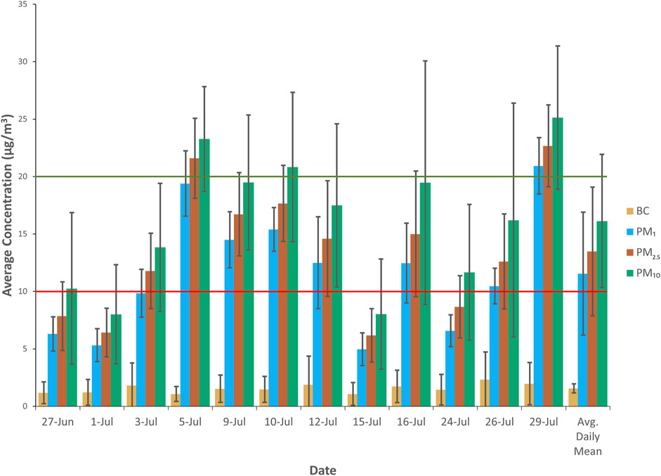
FIGURE 2. Daily mean concentrations of PM₁, PM_2.5, PM₁₀, and BC. Error bars represent standard deviations from the daily mean for each pollutant. The red horizontal line at 10 μg/m³ and the green horizontal line at 20 μg/m³ reflect World Health Organization guidelines for the lowest annual mean concentrations of PM_2.5 and PM₁₀, respectively, at which cardiopulmonary and lung cancer mortality increase with more than 95% confidence (World Health Organization, 2006).

FIGURE 3

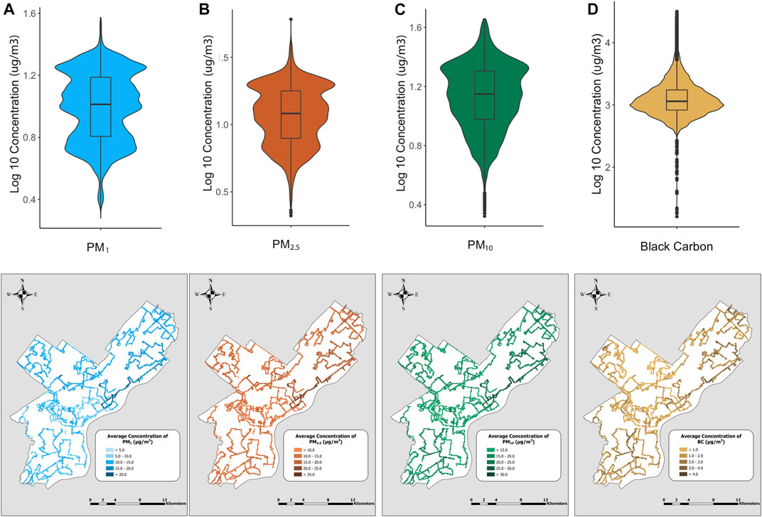
FIGURE 3. Violin plots and maps for (A) PM_1.(B) PM_2.5.(C) PM₁₀, and (D) BC. Violin plots show the distribution of all observed air pollutant concentrations on a log₁₀ scale, while maps show the overall average concentration of each pollutant in each 120 m² cell sampled over the data collection period.

FIGURE 4

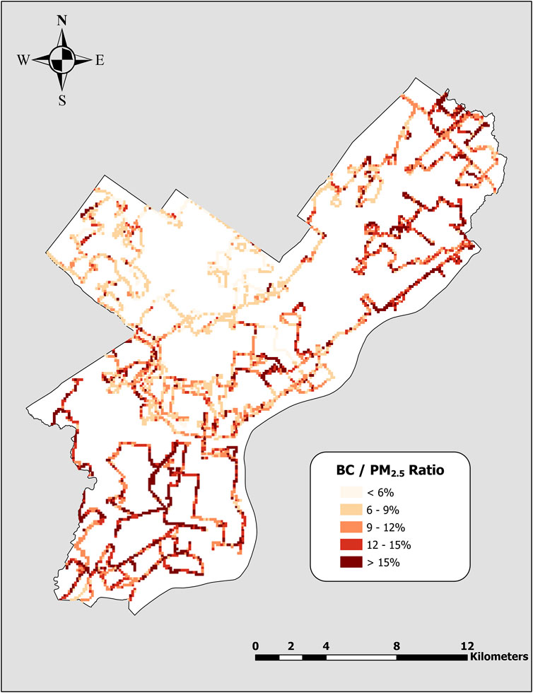
FIGURE 4. Daily average of the ratio of BC to fine PM (PM_2.5) in each 120 m² cell. BC/PM ratios are classified using quantiles.

FIGURE 5

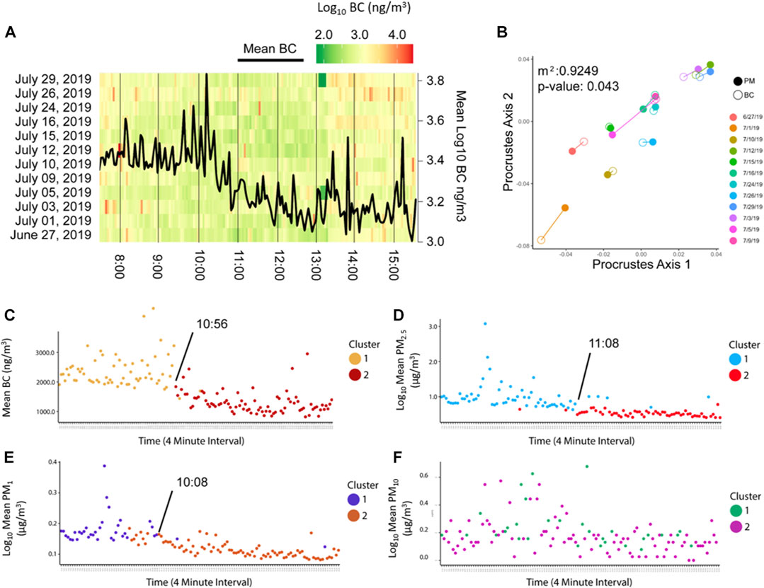
FIGURE 5. (A) Heatmap showing the log₁₀ concentration of BC across time (x-axis) and different days (y-axis). The black line reflects the log₁₀ mean concentration of BC averaged across all days. (B) Procrustes rotation ordination of correlation between BC and PM_2.5 on all days with correlation coefficient (m²) and a p-value. (C) Plot of log₁₀ mean BC concentration over time, colored by cluster, determined by k-means clustering. (D) Plot of log₁₀ mean PM_2.5 concentration over time, colored by cluster, determined by k-means clustering. (E) Plot of log₁₀ mean PM₁ concentration over time, colored by cluster, determined by k-means clustering. (F) Plot of log₁₀ mean PM₁₀ concentration over time, colored by cluster, determined by k-means clustering.

Statistically significant hotspots were found on all days across all measured size fractions of PM and BC throughout Philadelphia. The average concentrations of hotspots (Figure 6) within a given cell ranged from 8.7 ± 4.6 μg/m³ for BC; 18.7 ± 7.1 μg/m³ for PM₁; 28.0 ± 8.8 μg/m³ for PM_2.5; and 46.0 ± 17.3 μg/m³ for PM_10. All pollutants measured had hotspots that exhibited a tendency to recur in the same locations across multiple days; hotspots for PM₁ appeared in the same cell on as many as six separate days throughout the data collection period, while hotspots for PM_2.5, PM₁₀, and BC appeared in the same cell on up to five different days.

FIGURE 6

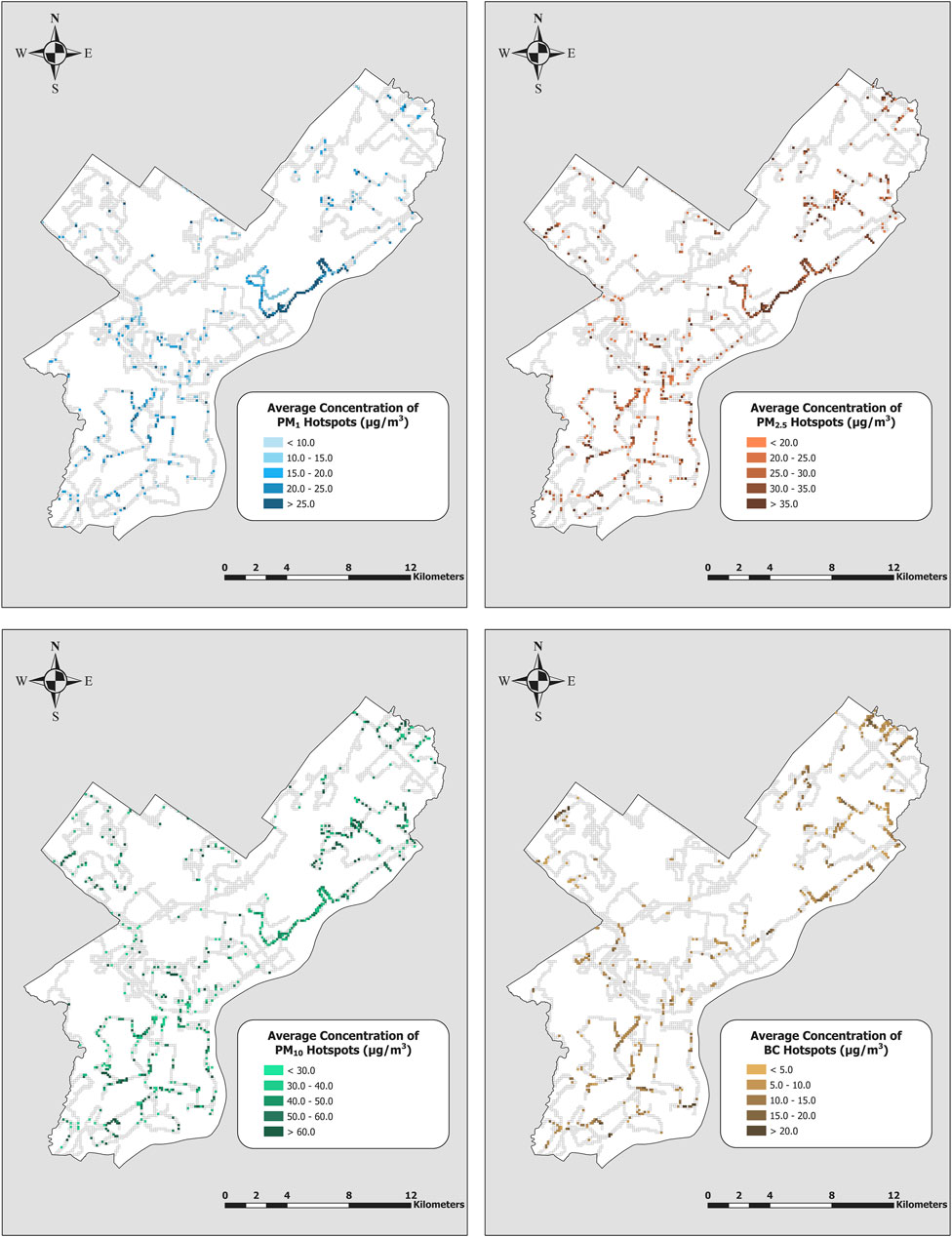
FIGURE 6. Maps displaying the locations and average concentrations of hotspots for PM₁ (top-left), PM_2.5 (top-right), PM₁₀ (bottom-left), and BC (bottom-right) in Philadelphia within each 120 m² cell sampled. Empty cells indicate that no hotspots were detected at that location.

Concentrations for all pollutants exhibited variation from day-to-day, with variation resulting from differences in weather conditions, traffic conditions, and slight deviations from the planned routes resulting from road closures (Figures 2, 7; Supplementary Tables S3–S6). All observations indicate the presence of PM 5 µm in diameter or smaller. PM exceeding 5 µm in diameter is not as ubiquitous throughout the data collection period, with larger particles not being detected at times throughout each day. Mass values observed for particles 1.6 µm diameter and larger generally demonstrated the greatest variation throughout each day, with particles with a diameter 0.5 µm and smaller also showing less within-day variation (Figure 7). The number, duration, and timing of PM_2.5 hotspots (Figure 7) varied from day to day; however, they were most consistently seen from 8:00–9:00 AM (30.19% of all hotspots) in complement with other studies where air pollutant concentrations peak during the morning hours (Zhao et al., 2009; Tunno et al., 2012).

FIGURE 7

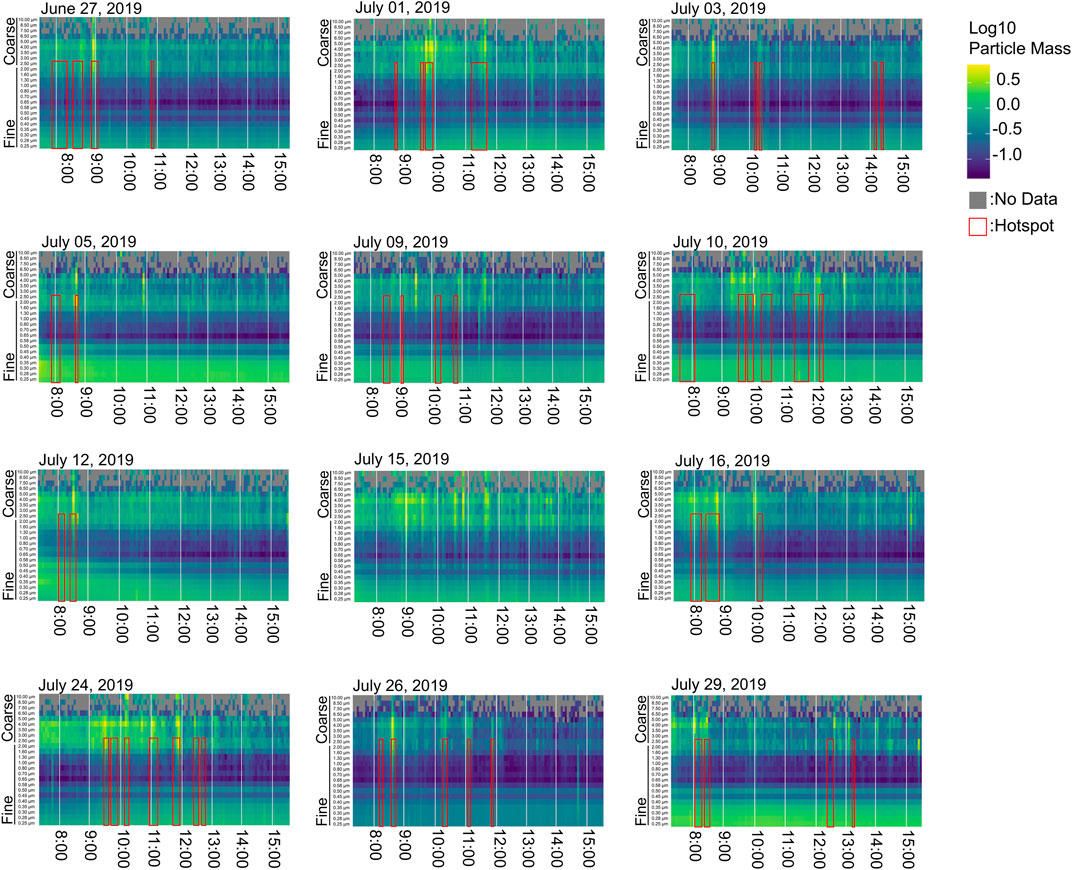
FIGURE 7. Heatmap of log₁₀ PM mass values across 24 fine and coarse size fractions throughout each day of data collection. Time of day is denoted on the x-axis. Hotspots for PM_2.5 fraction covering >2 min periods are identified by vertical red boxes. July 15, 2019 was excluded from hot spot analysis; as such, no hotspots are identified. As this is a large multi-panel image, we encourage the reader to download and zoom in if interested in particle mass concentrations of specific size fractions.

Discussion

Air pollution in Philadelphia is dominated by fine PM (PM_2.5). The PM_2.5/PM₁₀ ratio observed throughout the data collection period (83.6%) marks an increase relative to a stationary PM monitoring study that found that PM_2.5 only comprised 75% of PM in Philadelphia during the summers of 1992–1993 (Burton et al., 1996). The dominance of fine PM is reflected in the number of days that pollutant concentrations exceed their maximum annual recommended concentrations; while PM₁₀ exceeds recommended concentrations (20 μg/m³) on just 3 of the 12 sampling days, PM_2.5 exceeds its recommended concentration (10 μg/m³) on 8 sampling days. The prevalence of fine PM in Philadelphia suggests that anthropogenic sources are becoming increasingly large contributors to urban air pollution. Part of this increase may be due to the nature of on-road sampling itself; areas closer in proximity to roads tend to have higher concentrations of fine PM and lower concentrations of coarse PM relative to background sites due to the prevalence of traffic-related emissions (Barzyk et al., 2009; Karner et al., 2010; Yu et al., 2016). The increased proportion of finer PM may also result from changes within Philadelphia over time, such as urban development or increased traffic, that attenuate and/or remove potential sources of coarse PM while increasing potential sources of fine PM.

As BC and PM_2.5 are significantly correlated, the proportion of BC to overall fine PM in the air is helpful in determining the role of combustion processes in local pollution trends (Ni et al., 2014; Kim et al., 2017; Xu et al., 2017), which can in turn offer valuable information about potential sources of air pollutants in specific areas of urban environments. While the relationship between BC and fine PM in Philadelphia varies spatially (Figure 4) and temporally (Supplementary Figure S2), the overall BC/PM_2.5 ratio (11.6%) is comparable to BC/PM_2.5 ratios observed in other major cities, which range from 5–20% (Yu et al., 2015) and references therein). BC makes up a greater proportion of the measured PM_2.5 (Figure 4) in the North Delaware (NDEL) planning district, where heavy traffic conditions, proximity to major roads such as Interstate 95 (I-95), and local industry likely contribute to elevated BC concentrations. BC also makes up a significant fraction of PM_2.5 in the areas surrounding the Northeast Philadelphia Airport in RFNE and The Philadelphia International Airport in LSW, as landings and takeoffs by aircrafts at airports have been shown to increase local BC concentrations in the atmosphere (Agarwal et al., 2019). Pairwise comparison of BC and PM_2.5 concentrations revealed that the relationship between the two pollutants was generally variable from day to day (Supplementary Figure S2); variation in this relationship from day to day is due in part to the heterogeneity of emission sources and the urban landscape (Van den Bossche et al., 2015).

PM₁, PM_2.5, and PM₁₀ are spatially heterogenous and have similar spatial distributions throughout Philadelphia (Figure 3). The similarities that the PM_2.5 and PM₁ distributions share with the PM₁₀ distributions further demonstrate that most PM variation in Philadelphia can be characterized by changes in fine PM. Likewise, while there is slight variation in the location of hotspots among the different pollutants, the overall spatial distribution of hotspots throughout Philadelphia is similar across the three PM size fractions and BC (Figure 5). The areas with the highest frequency and concentration of hotspots are highly trafficked areas that are home to large public utility properties and heavy industry, which are likely significant sources of PM in this area (Philadelphia City Planning Commission, 2021). Relatively few hotspots were found in northern and western Philadelphia, which are located well outside of Philadelphia’s urban core. More open spaces have been shown to have a positive impact on air quality (Merbitz et al., 2012), and a previous study on air pollution in Philadelphia revealed associations between open spaces and low PM concentrations (Shakya et al., 2019). Traffic and industrial activity are less prominent in these areas relative to Philadelphia’s urban core, and a greater abundance of vegetation may curb air pollution primarily by uptake via leaf stomata and particle deposition (Beckett et al., 2000; Nowak et al., 2006).

The recurrence of hot spots in specific locations suggests that there are areas in Philadelphia where pollutant concentrations are consistently elevated relative to the surrounding area. A notable cluster of cells in the NDEL, RW, and NOR planning zones contain high concentration PM hotspots across multiple days. Other clusters of recurring hotspots are found within the University Southwest (USW) and LFNE planning zones. These hotspots are likely attributed to primary particles emitted from morning rush-hour traffic, where the number and density of vehicles on the road is higher relative to the rest of the day. The presence of hot spots outside the morning trend may be attributed to areas closer to industrial sites as in Chow et al., 1994, such as those located along the Interstate 676 (I-676) and I-95 corridors. While a substantial fraction of PM in urban areas originates from combustion engines, increased solar radiation during the summer months likely enhances the contribution of secondary particles formed from photooxidation of precursor molecules (Claeys et al., 2004; Shakya and Griffin, 2010) during the afternoon.

Temporal trends are evident in the concentration and distribution of PM₁, PM_2.5, and PM₁₀ from day to day (p < 0.05, Supplementary Tables S3–S5). Conversely, BC concentrations did not exhibit strong temporal variation (Supplementary Tables S6). The PM_2.5 size fraction (Figure 5D) clustered into two distinct time periods separated at approximately 11:08 AM, which complements our finding of BC clusters at approximately 10:56 AM (Figure 5C). Larger (PM₁₀) and smaller size (PM₁) fractions varied in their separation of peaks by time. PM₁ displayed less discrete temporal clustering (Figure 5E), with a break in clustering at approximately 10:08 AM. A cutoff was not found for PM₁₀. The lack of temporal clustering for PM₁₀, as seen in our results as well as a previous mobile monitoring study (Peters et al., 2013), affirms that coarse PM emission is relatively stochastic throughout the day, and may be attributed to the prevalence of crustal sources (e.g. dust resuspension) in areas that were sampled. These results complement findings in (Hankey and Marshall 2015), where PM size fractions were found to exhibit different concentrations in the morning and afternoon.

Limitations

Our analysis is limited by relatively few repetitions of routes over the course of a month in the summer. As our sampling occurs entirely on Philadelphia roadways, it should be noted that our measurements may be slightly different relative to ambient air further away from roads. More extensive sampling would allow for additional confidence in observed trends and provide opportunities to observe air pollution patterns at other temporal scales; sampling during late afternoon and evening hours would provide additional insight into air pollution trends throughout the day, while increased repetition of measurements both within and across seasons would allow for a seasonal analysis of air pollution trends (Liu et al., 2018). Likewise, we do not examine the precise impacts of wind speed/turbulence (Yang et al., 2020), temperature (Kalisa et al., 2018), and vegetation (Ottosen and Kumar, 2020) on air pollution distribution; discerning the influence of these factors on air pollution will further inform environmental policy and sustainable urban planning and design.

Conclusion

In this study, we demonstrate the potential for a mobile monitoring approach to assess the fine-scale spatiotemporal distribution of air pollutants throughout a major city. Our findings demonstrate the heterogeneity of PM and BC concentrations in space and time and show that finer PM comprises the majority of PM pollution in urban environments. Thus, measures that target fine PM emissions are paramount to reducing exposure to air pollution for residents of Philadelphia and other urban environments. Regulations and other efforts geared toward lowering PM emissions should be implemented on a city-wide scale, though hot spot analysis of PM and BC data reveal specific locations in Philadelphia (North, North Delaware, and River Wards planning districts) and times (morning hours) at which air pollution poses the greatest and most persistent threat to human health and wellbeing. These planning districts and the areas surrounding them merit further study throughout the year; as the recommended annual mean PM_2.5 concentration is exceeded on most sampling days, it is in the interest of public health to ascertain whether or not this trend is limited to the summer months. Should fine PM pollutant concentrations be chronically high throughout the year, individuals who are constantly exposed to the polluted air become more susceptible to cardiovascular and pulmonary damage. Additional consideration should be given to areas within these planning districts that are home to higher percentages of physiologically vulnerable (e.g. young, elderly, individuals with pre-existing conditions) and socioeconomically disadvantaged residents. It is crucial to address air quality problems in an environmentally just fashion to promote equitable urban sustainability, and further study in these areas can provide insight that can reduce disparities in the environmental health burden and improve overall human health in urban environments.

Though our analysis reveals spatiotemporal variation in PM and BC, along with possible causes of this variation, it stops short of estimating the contributions of specific sources to this variability; as our air pollution measurements covary in space and time, it is difficult to quantify the extent of variation resulting from spatial influences (locations of point sources, movement of non-point sources) and temporal influences (temporally sensitive atmospheric processes, random events) separately. Future analyses should consider the influence of urban composition and structure on air pollutant concentrations throughout cities. Cities can be quite different from each other compositionally and structurally, and the roles of urban structure (Cárdenas Rodríguez et al., 2016) and land use (Weng and Yang, 2006; Shakya et al., 2019) are important drivers of variation in urban air pollution. Cities can also vary significantly with regard to the regional climate; future studies of air pollution in Philadelphia and other urban environments should ascertain the influences of climate, specifically prevailing winds and temperature, on the spatiotemporal distribution of air pollutants. These analyses can be used to supplement existing knowledge regarding where and when air pollution may have the greatest adverse impacts on human and environmental health, which is essential to sustainable and equitable air quality management in our ever-expanding urban environments.

Data Availability Statement

The raw data supporting the conclusions of this article will be made available by the authors, without undue reservation. Data for PM and BC concentrations and GPS coordinates for hotspots can be accessed at https://github.com/Shakya-Kremer-Lab/AirPollution.

Author Contributions

Conceptualization: KS, PK. Data Collection: JS, RR, KS, PK. Formal Data Analysis: JS and LC, RR. Writing: LC, JS, RR, KS, PK. Supervision and Funding Acquisition: KS, PK.

Funding

Financial support for this study was provided through National Science Foundation (NSF) grant #1832407.

Conflict of Interest

The authors declare that the research was conducted in the absence of any commercial or financial relationships that could be construed as a potential conflict of interest.

Acknowledgments

We would like to thank Meghan Conway and Alexander Saad for their assistance in data collection.

Supplementary Material

The Supplementary Material for this article can be found online at: https://www.frontiersin.org/articles/10.3389/fbuil.2021.648620/full#supplementary-material

References

Abhijith, K. V., and Gokhale, S. (2015). Passive Control Potentials of Trees and On-Street Parked Cars in Reduction of Air Pollution Exposure in Urban Street Canyons. Environ. Pollut. 204, 99–108. doi:10.1016/j.envpol.2015.04.013

PubMed Abstract | CrossRef Full Text | Google Scholar

Agarwal, A., Speth, R. L., Fritz, T. M., Jacob, S. D., Rindlisbacher, T., Iovinelli, R., et al. (2019). SCOPE11 Method for Estimating Aircraft Black Carbon Mass and Particle Number Emissions. Environ. Sci. Technol. 53, 1364–1373. doi:10.1021/acs.est.8b04060

PubMed Abstract | CrossRef Full Text | Google Scholar

Aitchison, J., and Ho, C. H. (1989). The Multivariate Poisson-Log Normal Distribution. Biometrika 76 (4), 643–653. doi:10.1093/biomet/76.4.643

Apte, J. S., Messier, K. P., Gani, S., Brauer, M., Kirchstetter, T. W., Lunden, M. M., et al. (2017). High-Resolution Air Pollution Mapping with Google Street View Cars: Exploiting Big Data. Environ. Sci. Technol. 51 (12), 6999–7008. doi:10.1021/acs.est.7b00891

Barzyk, T. M., George, B. J., Vette, A. F., Williams, R. W., Croghan, C. W., and Stevens, C. D. (2009). Development of a Distance-to-Roadway Proximity Metric to Compare Near-Road Pollutant Levels to a Central Site Monitor. Atmos. Environ. 43 (4), 787–797. doi:10.1016/j.atmosenv.2008.11.002

Beckett, K. P., Freer-Smith, P. H., and Taylor, G. (2000). The Capture of Particulate Pollution by Trees at Five Contrasting Urban Sites. Arboricultural J. 24, 209–230. doi:10.1080/03071375.2000.9747273

CrossRef Full Text | Google Scholar

Brantley, H. L., Hagler, G. S. W., Kimbrough, E. S., Williams, R. W., Mukerjee, S., and Neas, L. M. (2014). Mobile Air Monitoring Data-Processing Strategies and Effects on Spatial Air Pollution Trends. Atmos. Meas. Tech. 7 (7), 2169–2183. doi:10.5194/amt-7-2169-2014

Burke, J. M., Zufall, M. J., and Özkaynak, H. (2001). A Population Exposure Model for Particulate Matter: Case Study Results for PM2.5 in Philadelphia, PA. J. Expo. Sci. Environ. Epidemiol. 11, 470–489. doi:10.1038/sj.jea.7500188

CrossRef Full Text | Google Scholar

Burton, R. M., Suh, H. H., and Koutrakis, P. (1996). Spatial Variation in Particulate Concentrations within Metropolitan Philadelphia. Environ. Sci. Technol. 30, 400–407. doi:10.1021/es950030f

CrossRef Full Text | Google Scholar

Cao, C., Jiang, W., Wang, B., Fang, J., Lang, J., Tian, G., et al. (2014). Inhalable Microorganisms in Beijing's PM2.5 and PM10 Pollutants during a Severe Smog Event. Environ. Sci. Technol. 48, 1499–1507. doi:10.1021/es4048472

PubMed Abstract | CrossRef Full Text | Google Scholar

Cárdenas Rodríguez, M., Dupont-Courtade, L., and Oueslati, W. (2016). Air Pollution and Urban Structure Linkages: Evidence from European Cities. Renew. Sustain. Energ. Rev. 53, 1–9. doi:10.1016/j.rser.2015.07.190

CrossRef Full Text | Google Scholar

Chow, J. C., Watson, J. G., Fujita, E. M., Lu, Z., Lawson, D. R., and Ashbaugh, L. L. (1994). Temporal and Spatial Variations of PM2.5 and PM10 Aerosol in the Southern California Air Quality Study. Atmos. Environ. 28, 2061–2080. doi:10.1016/1352-2310(94)90474-X

CrossRef Full Text | Google Scholar

City of PhiladelphiaDepartment of Public HealthAir Management Services (2019). Philadelphia’s Air Quality Report 2018. Available at: https://www.phila.gov/media/20191121163433/AQR_2018_Final.pdf (Accessed June 25, 2020).

Google Scholar

Claeys, M., Graham, B., Vas, G., Wang, W., Vermeylen, R., Pashynska, V., et al. (2004). Formation of Secondary Organic Aerosols Through Photooxidation of Isoprene. Science 303, 1173–1176. doi:10.1126/science.1092805

PubMed Abstract | CrossRef Full Text | Google Scholar

deSouza, P., Anjomshoaa, A., Duarte, F., Kahn, R., Kumar, P., and Ratti, C. (2020). Air Quality Monitoring Using Mobile Low-Cost Sensors Mounted on Trash-Trucks: Methods Development and Lessons Learned. Sustainable Cities Soc. 60, 102239. doi:10.1016/j.scs.2020.102239

Deville Cavellin, L., Weichenthal, S., Tack, R., Ragettli, M. S., Smargiassi, A., and Hatzopoulou, M. (2016). Investigating the Use of Portable Air Pollution Sensors to Capture the Spatial Variability of Traffic-Related Air Pollution. Environ. Sci. Technol. 50, 313–320. doi:10.1021/acs.est.5b04235

PubMed Abstract | CrossRef Full Text | Google Scholar

Dockery, D. W., Pope, C. A., Xu, X., Spengler, J. D., Ware, J. H., Fay, M. E., et al. (1993). An Association between Air Pollution and Mortality in Six U.S. Cities. N. Engl. J. Med. 329, 1753–1759. doi:10.1056/NEJM199312093292401

PubMed Abstract | CrossRef Full Text | Google Scholar

Dominici, F., Peng, R. D., Bell, M. L., Pham, L., McDermott, A., Zeger, S. L., et al. (2006). Fine Particulate Air Pollution and Hospital Admission for Cardiovascular and Respiratory Diseases. JAMA 295, 1127–1134. doi:10.1001/jama.295.10.1127

PubMed Abstract | CrossRef Full Text | Google Scholar

Gallagher, J., Baldauf, R., Fuller, C. H., Kumar, P., Gill, L. W., and McNabola, A. (2015). Passive Methods for Improving Air Quality in the Built Environment: A Review of Porous and Solid Barriers. Atmos. Environ. 120, 61–70. doi:10.1016/j.atmosenv.2015.08.075

Getis, A., and Ord, J. K. (1992). The Analysis of Spatial Association by Use of Distance Statistics. Geographical Anal. 24, 189–206. doi:10.1111/j.1538-4632.1992.tb00261.x

CrossRef Full Text | Google Scholar

Gotelli, N. J., and Ellison, A. M. (2004). A primer of ecological statistics. Sunderland, MA: Sinauer Associates Publishers.

Gozzi, F., Della Ventura, G., and Marcelli, A. (2016). Mobile Monitoring of Particulate Matter: State of Art and Perspectives. Atmos. Pollut. Res. 7, 228–234. doi:10.1016/j.apr.2015.09.007

CrossRef Full Text | Google Scholar

Gray, S. C., Edwards, S. E., and Miranda, M. L. (2013). Race, Socioeconomic Status, and Air Pollution Exposure in North Carolina. Environ. Res. 126, 152–158. doi:10.1016/j.envres.2013.06.005

PubMed Abstract | CrossRef Full Text | Google Scholar

Gromke, C., and Ruck, B. (2012). Pollutant Concentrations in Street Canyons of Different Aspect Ratio with Avenues of Trees for Various Wind Directions. Boundary Layer Meteorol. 144 (1), 41–64. doi:10.1007/s10546-012-9703-z

Hagler, G. S. W., Lin, M. Y., Khlystov, A., Baldauf, R. W., Isakov, V., Faircloth, J., et al. (2012). Field Investigation of Roadside Vegetative and Structural Barrier Impact on Near-Road Ultrafine Particle Concentrations Under a Variety of Wind Conditions. Sci. Total Environ. 419, 7–15. doi:10.1016/j.scitotenv.2011.12.002

Hamstead, Z. A., Kremer, P., Larondelle, N., McPhearson, T., and Haase, D. (2016). Classification of the Heterogeneous Structure of Urban Landscapes (STURLA) as an Indicator of Landscape Function Applied to Surface Temperature in New York City. Ecol. Indicators 70, 574–585. doi:10.1016/j.ecolind.2015.10.014

CrossRef Full Text | Google Scholar

Hankey, S., and Marshall, J. D. (2015). On-bicycle Exposure to Particulate Air Pollution: Particle Number, Black Carbon, PM 2.5, and Particle Size. Atmos. Environ. 122, 65–73. doi:10.1016/j.atmosenv.2015.09.025

CrossRef Full Text | Google Scholar

Hussein, T., Johansson, C., Karlsson, H., and Hansson, H-C. (2008). Factors Affecting Non-tailpipe Aerosol Particle Emissions from Paved Roads: On-Road Measurements in Stockholm, Sweden. Atmos. Environ. 42, 688–702. doi:10.1016/j.atmosenv.2007.09.064

CrossRef Full Text | Google Scholar

Kalisa, E., Fadlallah, S., Amani, M., Nahayo, L., and Habiyaremye, G. (2018). Temperature and Air Pollution Relationship During Heatwaves in Birmingham, UK. Sustainable Cities Soc. 43, 111–120. doi:10.1016/j.scs.2018.08.033

Karner, A. A., Eisinger, D. S., and Niemeier, D. A. (2010). Near-Roadway Air Quality: Synthesizing the Findings from Real-World Data. Environ. Sci. Technol. 44 (14), 5334–5344. doi:10.1021/es100008x

Kelly, F. J., and Fussell, J. C. (2012). Size, Source and Chemical Composition as Determinants of Toxicity Attributable to Ambient Particulate Matter. Atmos. Environ. 60, 504–526. doi:10.1016/j.atmosenv.2012.06.039

CrossRef Full Text | Google Scholar

Kim, S., Yu, S., and Yun, D. (2017). Spatiotemporal Association of Real-Time Concentrations of Black Carbon (BC) with Fine Particulate Matters (PM2.5) in Urban Hotspots of South Korea. Int. J. Environ. Res. Public Health 14, 1350. doi:10.3390/ijerph14111350

PubMed Abstract | CrossRef Full Text | Google Scholar

Likas, A., Vlassis, N., and Verbeek, J. J. (2003). The Global K-Means Clustering Algorithm. Pattern Recognit. 36 (2), 451–461. doi:10.1016/S0031-3203(02)00060-2

CrossRef Full Text | Google Scholar

Liu, Y., Wu, J., Yu, D., and Ma, Q. (2018). The Relationship between Urban Form and Air Pollution Depends on Seasonality and City Size. Environ. Sci. Pollut. Res. 25, 15554–15567. doi:10.1007/s11356-018-1743-6

PubMed Abstract | CrossRef Full Text | Google Scholar

Miller, F. J., Gardner, D. E., Graham, J. A., Lee, R. E., Wilson, W. E., and Bachmann, J. D. (1979). Size Considerations for Establishing a Standard for Inhalable Particles. J. Air Pollut. Control. Assoc. 29, 610–615. doi:10.1080/00022470.1979.10470831

CrossRef Full Text | Google Scholar

Ni, M., Huang, J., Lu, S., Li, X., Yan, J., and Cen, K. (2014). A Review on Black Carbon Emissions, Worldwide and in China. Chemosphere 107, 83–93. doi:10.1016/j.chemosphere.2014.02.052

PubMed Abstract | CrossRef Full Text | Google Scholar

Nowak, D. J., Crane, D. E., and Stevens, J. C. (2006). Air Pollution Removal by Urban Trees and Shrubs in the United States. Urban For. Urban Green. 4, 115–123. doi:10.1016/j.ufug.2006.01.007

CrossRef Full Text | Google Scholar

Ottosen, T. B., and Kumar, P. (2020). The Influence of the Vegetation Cycle on the Mitigation of Air Pollution by a Deciduous Roadside Hedge. Sustainable Cities Soc. 53, 101919. doi:10.1016/j.scs.2019.101919

Paul, G., Nolen, J. E., Alexander, L., Bender, L. K., Vleet, V., Barrett, W., et al. (2019). American Lung Association State of the Air 2019. Available at: https://www.stateoftheair.org/assets/sota-2019-full.pdf (Accessed June 25, 2020).

Perlin, S. A., Sexton, K., and Wong, D. W. S. (1999). An Examination of Race and Poverty for Populations Living Near Industrial Sources of Air Pollution. J. Expo. Sci. Environ. Epidemiol. 9 (1), 29–48. doi:10.1038/sj.jea.7500024

CrossRef Full Text | Google Scholar

Peters, J., Theunis, J., Poppel, M. V., and Berghmans, P. (2013). Monitoring PM10 and Ultrafine Particles in Urban Environments Using Mobile Measurements. Aerosol Air Qual. Res. 13, 509–522. doi:10.4209/aaqr.2012.06.0152

CrossRef Full Text | Google Scholar

Philadelphia City Planning Commission (2021). Philadelphia2035. Available at: https://www.phila2035.org/ (Accessed July 24, 2020).

Google Scholar

Rabinovitch, N., Strand, M., and Gelfand, E. W. (2006). Particulate Levels Are Associated with Early Asthma Worsening in Children with Persistent Disease. Am. J. Respir. Crit. Care Med. 173, 1098–1105. doi:10.1164/rccm.200509-1393OC

PubMed Abstract | CrossRef Full Text | Google Scholar

Salmond, J. A., Williams, D. E., Laing, G., Kingham, S., Dirks, K., Longley, I., et al. (2013). The Influence of Vegetation on the Horizontal and Vertical Distribution of Pollutants in a Street Canyon. Sci. Total Environ. 443, 287–298. doi:10.1016/j.scitotenv.2012.10.101

Shakya, K. M., and Griffin, R. J. (2010). Secondary Organic Aerosol from Photooxidation of Polycyclic Aromatic Hydrocarbons. Environ. Sci. Technol. 44, 8134–8139. doi:10.1021/es1019417

PubMed Abstract | CrossRef Full Text | Google Scholar

Shakya, K. M., Rupakheti, M., Aryal, K., and Peltier, R. E. (2016). Respiratory Effects of High Levels of Particulate Exposure in a Cohort of Traffic Police in Kathmandu, Nepal. J. Occup. Environ. Med. 58, e218–e225. doi:10.1097/JOM.0000000000000753

PubMed Abstract | CrossRef Full Text | Google Scholar

Shakya, K. M., Kremer, P., Henderson, K., McMahon, M., Peltier, R. E., Bromberg, S., et al. (2019). Mobile Monitoring of Air and Noise Pollution in Philadelphia Neighborhoods during Summer 2017. Environ. Pollut. 255, 113195. doi:10.1016/j.envpol.2019.113195

PubMed Abstract | CrossRef Full Text | Google Scholar

Sm, S. N., Reddy Yasa, P., Mv, N., Khadirnaikar, S., and Pooja, R. (2019). Mobile Monitoring of Air Pollution Using Low Cost Sensors to Visualize Spatio-Temporal Variation of Pollutants at Urban Hotspots. Sustainable Cities Soc. 44, 520–535. doi:10.1016/j.scs.2018.10.006

Stewart, J. D., Kremer, P., Shakya, K. M., Conway, M., and Saad, A. (2021). Outdoor Atmospheric Microbial Diversity Is Associated with Urban Landscape Structure and Differs from Indoor-Transit Systems as Revealed by Mobile Monitoring and Three-Dimensional Spatial Analysis. Front. Ecol. Evol. 9, 1–12. doi:10.3389/fevo.2021.620461

CrossRef Full Text | Google Scholar

Strosnider, H., Kennedy, C., Monti, M., and Yip, F. (2017). Rural and Urban Differences in Air Quality, 2008-2012, and Community Drinking Water Quality, 2010-2015 - United States. MMWR Surveill. Summ. 66, 1–10. doi:10.15585/mmwr.ss6613a1

PubMed Abstract | CrossRef Full Text | Google Scholar

Targino, A. C., Gibson, M. D., Krecl, P., Rodrigues, M. V. C., dos Santos, M. M., and de Paula Corrêa, M. (2016). Hotspots of Black Carbon and PM2.5 in an Urban Area and Relationships to Traffic Characteristics. Environ. Pollut. 218, 475–486. doi:10.1016/j.envpol.2016.07.027

PubMed Abstract | CrossRef Full Text | Google Scholar

Ten Berge, J. M. F. (1977). Orthogonal Procrustes Rotation for Two or More Matrices. Psychometrika 42, 267–276. doi:10.1007/BF02294053

CrossRef Full Text | Google Scholar

Tsapakis, M., Lagoudaki, E., Stephanou, E. G., Kavouras, I. G., Koutrakis, P., Oyola, P., et al. (2002). The Composition and Sources of PM2.5 Organic Aerosol in Two Urban Areas of Chile. Atmos. Environ. 36, 3851–3863. doi:10.1016/S1352-2310(02)00269-8

CrossRef Full Text | Google Scholar

Tunno, B. J., Shields, K. N., Lioy, P., Chu, N., Kadane, J. B., Parmanto, B., et al. (2012). Understanding Intra-neighborhood Patterns in PM2.5 and PM10 Using Mobile Monitoring in Braddock, PA. Environ. Health 11, 76. doi:10.1186/1476-069X-11-76

PubMed Abstract | CrossRef Full Text | Google Scholar

United Nations (2019). Department of Economic and Social Affairs, Population DivisionWorld Urbanization Prospects: The 2018 Revision. New York: United Nations.

United States Environmental Protection Agency (2015). Report on the Environment (ROE)–Particulate Matter Emissions. Available at: https://cfpub.epa.gov/roe/indicator.cfm?i=19 (Accessed July 24, 2020).

Google Scholar

Vallius, M., Janssen, N. A. H., Heinrich, J., Hoek, G., Ruuskanen, J., Cyrys, J., et al. (2005). Sources and Elemental Composition of Ambient PM2.5 in Three European Cities. Sci. Total Environ. 337, 147–162. doi:10.1016/j.scitotenv.2004.06.018

PubMed Abstract | CrossRef Full Text | Google Scholar

Van den Bossche, J., Peters, J., Verwaeren, J., Botteldooren, D., Theunis, J., and De Baets, B. (2015). Mobile Monitoring for Mapping Spatial Variation in Urban Air Quality: Development and Validation of a Methodology Based on an Extensive Dataset. Atmos. Environ. 105, 148–161. doi:10.1016/j.atmosenv.2015.01.017

CrossRef Full Text | Google Scholar

Van Poppel, M., Peters, J., and Bleux, N. (2013). Methodology for Setup and Data Processing of Mobile Air Quality Measurements to Assess the Spatial Variability of Concentrations in Urban Environments. Environ. Pollut. 183, 224–233. doi:10.1016/j.envpol.2013.02.020

PubMed Abstract | CrossRef Full Text | Google Scholar

Weng, Q., and Yang, S. (2006). Urban Air Pollution Patterns, Land Use, and Thermal Landscape: An Examination of the Linkage Using GIS. Environ. Monit. Assess. 117, 463–489. doi:10.1007/s10661-006-0888-9

PubMed Abstract | CrossRef Full Text | Google Scholar

World Health Organization (2006). WHO Air Quality Guidelines for Particulate Matter, Ozone, Nitrogen Dioxide and Sulfur Dioxide, Global Update 2005. Copenhagen, Denmark: WHO Regional Office for Europe.

World Health Organization (2018). 9 Out of 10 People Worldwide Breathe Polluted Air, but More Countries Are Taking Action. Geneva: News releaseAvailable at: https://www.who.int/news/item/02-05-2018-9-out-of-10-people-worldwide-breathe-polluted-air-but-more-countries-are-taking-action (Accessed December 1, 2020).

Xing, Y., and Brimblecombe, P. (2019). Role of Vegetation in Deposition and Dispersion of Air Pollution in Urban Parks. Atmos. Environ. 201 (December 2018), 73–83. doi:10.1016/j.atmosenv.2018.12.027

Xu, G., Jiao, L., Zhang, B., Zhao, S., Yuan, M., Gu, Y., et al. (2017). Spatial and Temporal Variability of the PM2.5/PM10 Ratio in Wuhan, Central China. Aerosol Air Qual. Res. 17, 741–751. doi:10.4209/aaqr.2016.09.0406

CrossRef Full Text | Google Scholar

Yang, J., Shi, B., Shi, Y., Marvin, S., Zheng, Y., and Xia, G. (2020). Air Pollution Dispersal in High Density Urban Areas: Research on the Triadic Relation of Wind, Air Pollution, and Urban Form. Sustainable Cities Soc. 54, 101941. doi:10.1016/j.scs.2019.101941

Yu, N., Zhu, Y., Xie, X., Yan, C., Zhu, T., and Zheng, M. (2015). Characterization of Ultrafine Particles and Other Traffic Related Pollutants Near Roadways in Beijing. Aerosol Air Qual. Res. 15, 1261–1269. doi:10.4209/aaqr.2014.11.0295

CrossRef Full Text | Google Scholar

Yu, C. H., Fan, Z., Lioy, P. J., Baptista, A., Greenberg, M., and Laumbach, R. J. (2016). A Novel Mobile Monitoring Approach to Characterize Spatial and Temporal Variation in Traffic-Related Air Pollutants in an Urban Community. Atmos. Environ. 141, 161–173. doi:10.1016/j.atmosenv.2016.06.044

CrossRef Full Text | Google Scholar

Zhang, M. L., and Zhou, Z. H. (2005). A k-nearest neighbor-based algorithm for multi-label classification. 2005 IEEE International Conference on Granular Computing, Beijing, China, July 25–27, 2005 (IEEE) 2, 718–721. doi:10.1109/GRC.2005.1547385

Zhang, Y-L., and Cao, F. (2015). Fine Particulate Matter (PM2.5) in China at a City Level. Sci. Rep. 5, 14884. doi:10.1038/srep14884

PubMed Abstract | CrossRef Full Text | Google Scholar

Zhang, A., Qi, Q., Jiang, L., Zhou, F., and Wang, J. (2013). Population Exposure to PM2.5 in the Urban Area of Beijing. PLOS ONE 8, e63486. doi:10.1371/journal.pone.0063486

PubMed Abstract | CrossRef Full Text | Google Scholar

Zhao, X., Zhang, X., Xu, X., Xu, J., Meng, W., and Pu, W. (2009). Seasonal and Diurnal Variations of Ambient PM2.5 Concentration in Urban and Rural Environments in Beijing. Atmos. Environ. 43, 2893–2900. doi:10.1016/j.atmosenv.2009.03.009

CrossRef Full Text | Google Scholar

Zhou, Z., Dionisio, K. L., Arku, R. E., Quaye, A., Hughes, A. F., Vallarino, J., et al. (2011). Household and Community Poverty, Biomass Use, and Air Pollution in Accra, Ghana. Proc. Natl. Acad. Sci. 108 (27), 11028–11033. doi:10.1073/pnas.1019183108

PubMed Abstract | CrossRef Full Text | Google Scholar