Estimation of Ground Profiles Based on Microtremor Survey in the Bangkok Basin

Introduction

Bangkok, the capital city of the Kingdom of Thailand, is the major economic hub of the region. The Bangkok Metropolitan Region, comprising of Bangkok and five adjacent provinces, covers an area of 7,762 km². It is densely populated, with more than 14 million people according to the 2010 census (City Population, 2019). Bangkok lies in the central region of Thailand which is a low seismicity zone. Small and moderate-sized earthquakes have occurred about 150 km from Bangkok. Larger magnitude earthquakes are generated by the highly active Sumatra fault system located more than 400 km from Bangkok (Ornthammarath et al., 2010). Moderate-size earthquakes are frequent along the northern and north-western boundary of Thailand and Myanmar. Although Bangkok is situated far from the epicenters of historical earthquake events and does not have a history of major earthquake damage, many earthquakes have been felt in high-rise buildings in the city. In 1983, an earthquake of body-wave magnitude (m_b) 5.8 occurred in the Srinakarin Reservoir, the epicenter being ∼200 km from Bangkok. The earthquake was felt strongly in Bangkok and caused minor damage in some buildings (Baoqi and Renfa, 1990). It caused panic among Bangkok residents. The Three Pagodas fault zone and Sri Sawat fault zone are major fault systems in the Kanchanaburi province. There were no reported earthquakes related to these faults, thus they were considered inactive before the construction of the water reservoirs (Pananont et al., 2011). The study reports that the impoundment of the reservoirs triggered seismicity in the region and currently the fault systems show dextral movement. The location of the fault systems relative to Bangkok is presented in the study by the Department of Mineral Resources Thailand [DMR (Department of Mineral Resources), 2006]. Lukkunaprasit (1993) reports that the 1988 earthquake in southern China (near the Myanmar border, 1,000 km from Bangkok) with a Richter magnitude of 7.3 was felt in high-rise buildings in Bangkok. The study lists many earthquakes felt in high-rise buildings in Bangkok despite the large epicentral distances. In recent times, the epicenter of the 2011 Mw 6.8 Tarlay (Myanmar) earthquake was 775 km from Bangkok. The 2014 Mae Lao (Thailand) earthquake of Mw 6.1 occurred at an epicentral distance of 670 km from Bangkok. Both earthquakes were felt in high-rise buildings in the capital (Ornthammarath, 2013, Ornthammarath and Warnitchai, 2016).

The Thai Meteorological Department (TMD) seismic station is located at (13.67′N, 100.61′E) in the Bangkok basin (Figure 1). TMD recorded the 2008 Mw 7.9 Sichuan earthquake, 2011 Tarlay (Myanmar) earthquake and the 2014 Mae Lao (Thailand) earthquake. The 2008 earthquake was also recorded by the SRTD station at (14.39′N, 99.12′E) which is a rocky site outside the Bangkok basin with no sediment deposit. The acceleration time history, Fourier spectra and horizontal-to-vertical (HV) ratio of Fourier spectrum of the three earthquakes are shown in Figure 2. The HV ratio of the Sichuan earthquakes at TMD shows a clear peak at 0.2 Hz (Figure 2A). Note that in 2008, the sensors at TMD were placed 40 m below the ground surface. For the same earthquake event, the SRTD records (Figure 2B) do not show the low-frequency peak. Both the 2011 Tarlay earthquake (Figure 2C) and 2014 Mae Lao earthquake (Figure 2D) show similar peaks.

FIGURE 1

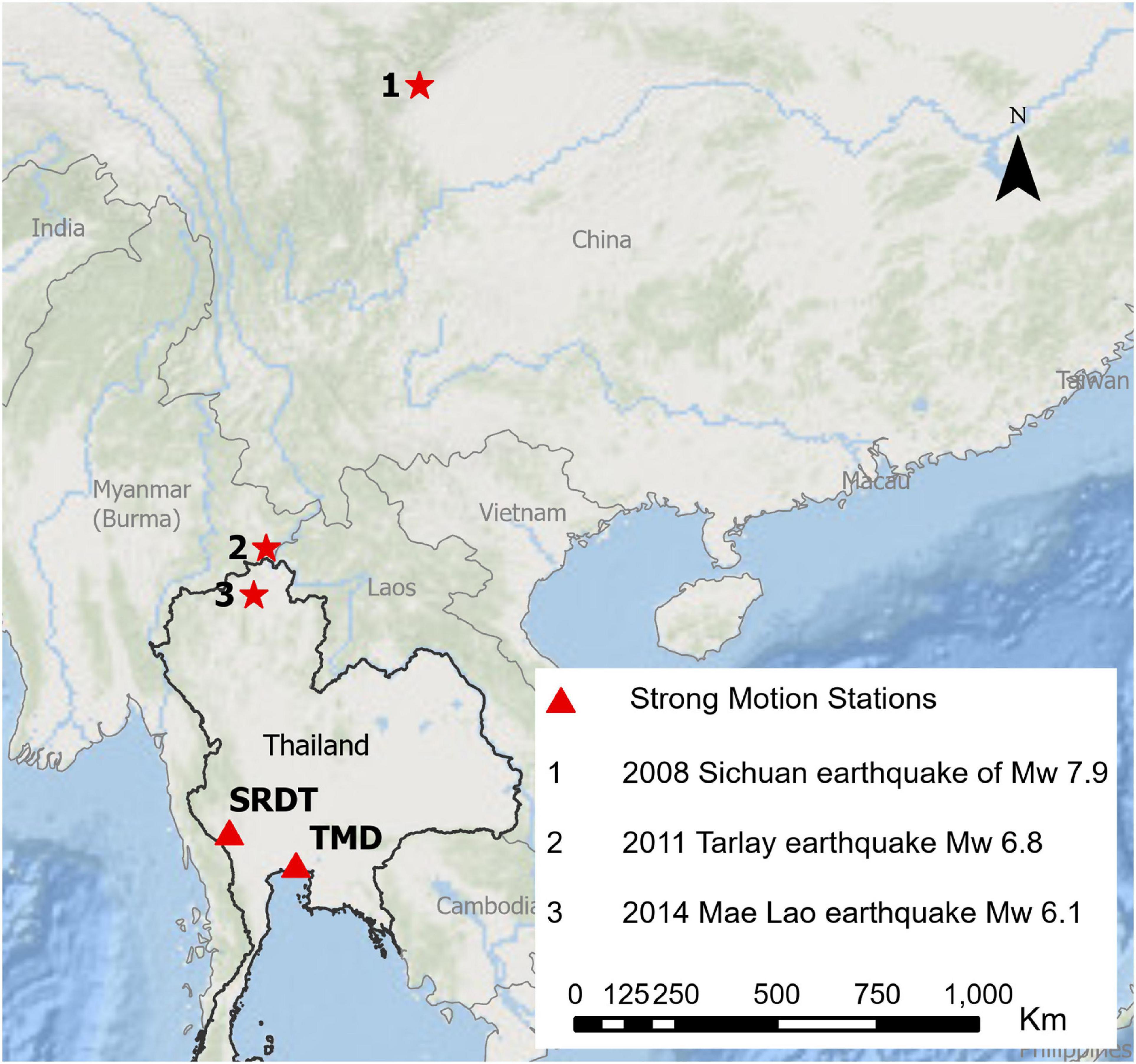
Figure 1. Location of strong-motion stations TMD and SRDT with respect to the epicenter of the 2008 Sichuan Earthquake, 2011 Tarlay (Myanmar) earthquake and 2014 Mae Lao (Thailand) earthquake.

FIGURE 2

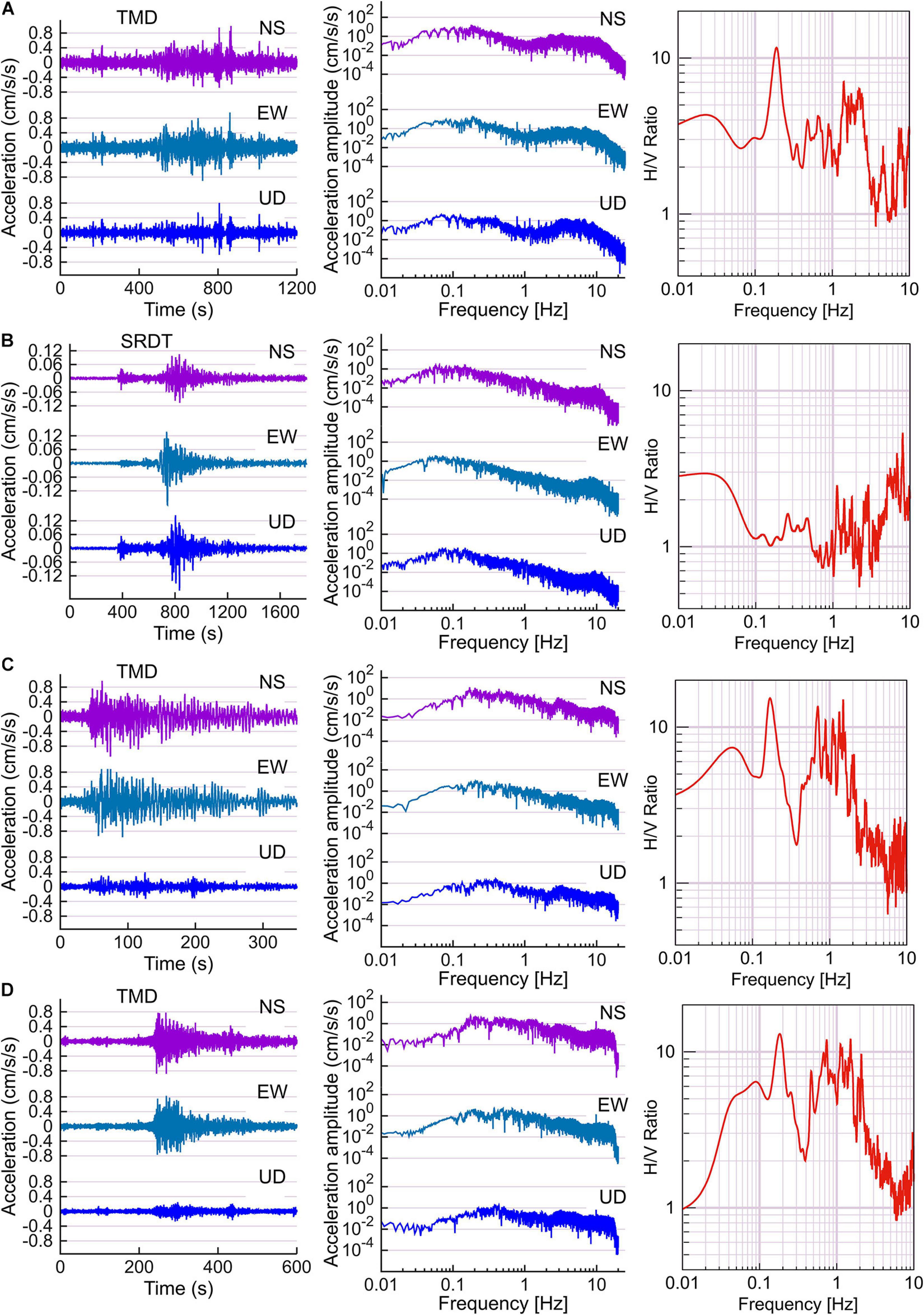
Figure 2. Acceleration time history, Fourier spectra, and horizontal to vertical spectral ratio at (A) TMD station from the 2008 Sichuan Earthquake with sensor located 40 m below the ground surface, (B) SRDT station from the 2008 Sichuan Earthquake. (C) TMD station from the 2011 Tarlay (Myanmar) earthquake and (D) the 2014 Mae Lao (Thailand) earthquake.

Bangkok lies on soft alluvial deposits in a deep basin; these conditions amplify long-period seismic waves. Despite the absence of major seismic damage so far, the risk of seismic damage in Bangkok is rising due to a growing number of structures susceptible to low-frequency seismic waves, especially high-rise and super high-rise buildings. Most of the research on seismic risk in Bangkok is focused on the high-frequency ranges and shallow ground profiles. Therefore, it is important to determine the predominant period in the long-period seismic range and study deep soil profiles.

Geological Setting

The central plain of Thailand is a wide depositional flat plain and can be divided into upper and lower regions. The lower region, called the Lower Central plain or Chao Phraya plain, extends from Chainat province in the north at (15°15′N, 100°15′E) to the Gulf of Thailand at Samut Prakan (13°30′N, 100°30′E) in the south (Sinsakul, 2000). The approximate distance from Chainat, where the Chao-Phraya river transcends to its estuary in the flat plain is 200 km. The east–west distance at the widest part of the plain is around 180 km. The total area of the lower central plain is approximately 36,000 km². The plain is flat with elevation above sea level ranging from 1.5 m at Bangkok, 2.5 m at Ayutthaya, and 15 m at Chainat. The plain encompasses the Bangkok metropolitan region.

The lower central plain is bounded by the Khorat Plateau on the east and the western mountain ranges on the west, with fault scarps as the margins. The basement is a graben formed by block faulting in the late Pliocene–Pleistocene, primarily trending in north-south direction (Sinsakul, 2000; Phien-wej et al., 2006). The pre-Quaternary geology consists of the basement of sedimentary, igneous, and metamorphic rocks from Paleozoic to Mesozoic eras and tertiary rocks above the basement characterized by claystone, siltstone, sandstone, and conglomerate. The Quaternary geology includes thick accumulation of unconsolidated Pleistocene and Holocene sediments. The top eight layers of the sediments are commonly known as the Bangkok aquifer system, which are separated from each other by confining clay or sandy clay layers (Sinsakul, 2000). Late Quaternary geology includes sedimentary succession of the Chao Phraya Delta with the riverine and marine deposits during Late Pleistocene to Holocene epochs. A soft clay layer was deposited during the Holocene epoch when the Plain was covered by sea. Regression started at around 6,000 years B.P. and reached the present level at around 1,500 years B.P. The soft clay covers 13,800 km² area of the Plain and is commonly known as the Bangkok clay (Sinsakul, 2000; Phien-wej et al., 2006).

The Lower Central Plain has a largely irregular basement and tertiary rocks at depths of 500–2,000 m beneath the sediment layers (Sinsakul, 2000). There are only a few deep boreholes reaching the basement rocks. In most parts of the city a layer of soft clay is found at depths of 12–16 m, in some areas even exceeding 20 m in depth (Phien-wej et al., 2006). Drilling carried out for water and oil prospecting and seismic reflection surveys show that the basement of the Bangkok metropolitan area is deep and irregular. Phien-wej et al. (2006) reports that the basement depth changes from 2,100 to 450 m from the mouth of the Chao-Phraya river to a nearby point to the east. In the northeast side the depth is 600 m and the southwestern area extends down to 1,900 m. The paper does not give the exact location of these points. Above the basement, there are complex layers of alluvial sandy soil and deltaic clay or silt. The sequence of aquifers and clay deposits in the upper 450 m of the basin are well known (Phien-wej et al., 2006); however, the deeper profiles are not well established.

Microtremor Data Recording

Conventional methods to determine the shear-wave velocity (Vs) of soil deposits include seismic refraction surveys and surface-wave surveys, down-hole measurements in boreholes, cross-hole surveys and laboratory tests. Among these, the first two methods are non-intrusive. When the sedimentary deposits are deep, borehole measurements require deep drilling which increases cost and reduces the accuracy. The Microtremor Survey Method (MSM) is more effective than conventional seismic methods in heavily populated urban areas like Bangkok because of its non-intrusiveness, ease of use, shorter preparation and recording time, and better portability. It is economic as well as environmentally friendly and does not require any laboratory tests beforehand. MSM uses ambient ground-motion recordings for shallow or deep subsurface exploration. Papadopoulos et al. (2017) used analysis of single point and array measurements of ambient vibration to determine the subsurface geophysical properties in the Chania basin–a basin with a similar geological complexity as the study area.

A microtremor survey was carried out in Bangkok from July 14th to July 17th, 2019 during the holiday season in the daytime. Data were recorded at five sites (see details and locations in Table 1 and Figure 3). Each 4-point array comprised of simultaneous recording by three instruments placed along the circumference of a circle and one at the center. Various radius sizes were used at each site during the survey. Figure 4 shows the array configuration at site CU. The instruments used for the survey are four sets of microtremor recorders DATAMARK JU410 by HAKUSAN Co., Ltd., (JU410), four sets of Mini Seismometers HS-1 by OYO SI (HS-1) and one set of Data loggers HKS-9700 by Keisokugiken Corporation.

TABLE 1

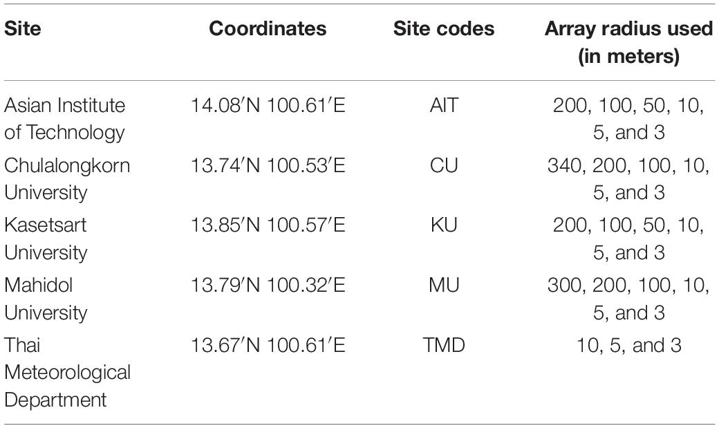
Table 1. Details of the seismic survey sites.

FIGURE 3

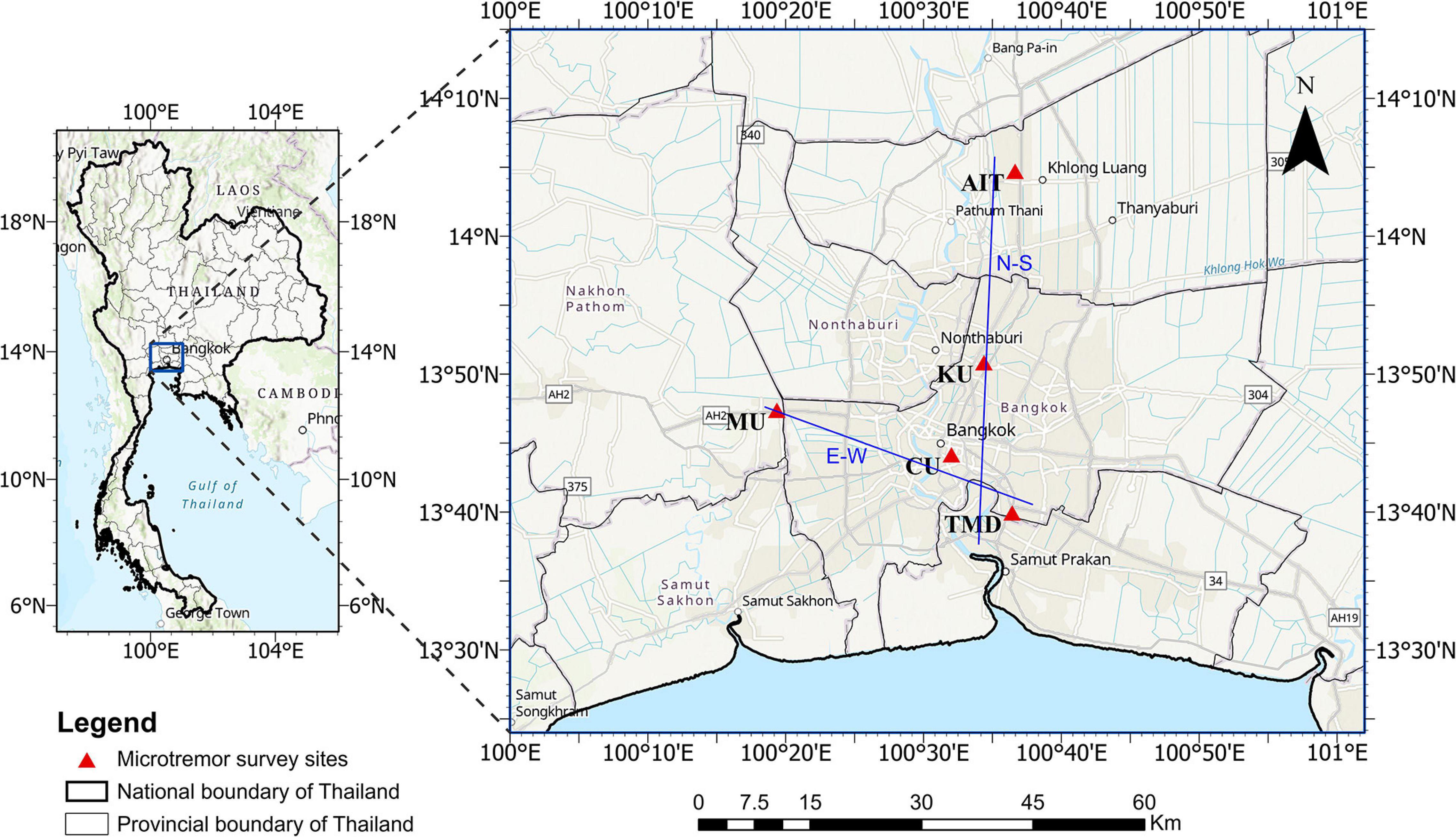
Figure 3. Left: Location of Bangkok in Thailand. Right: Location of survey stations.

FIGURE 4

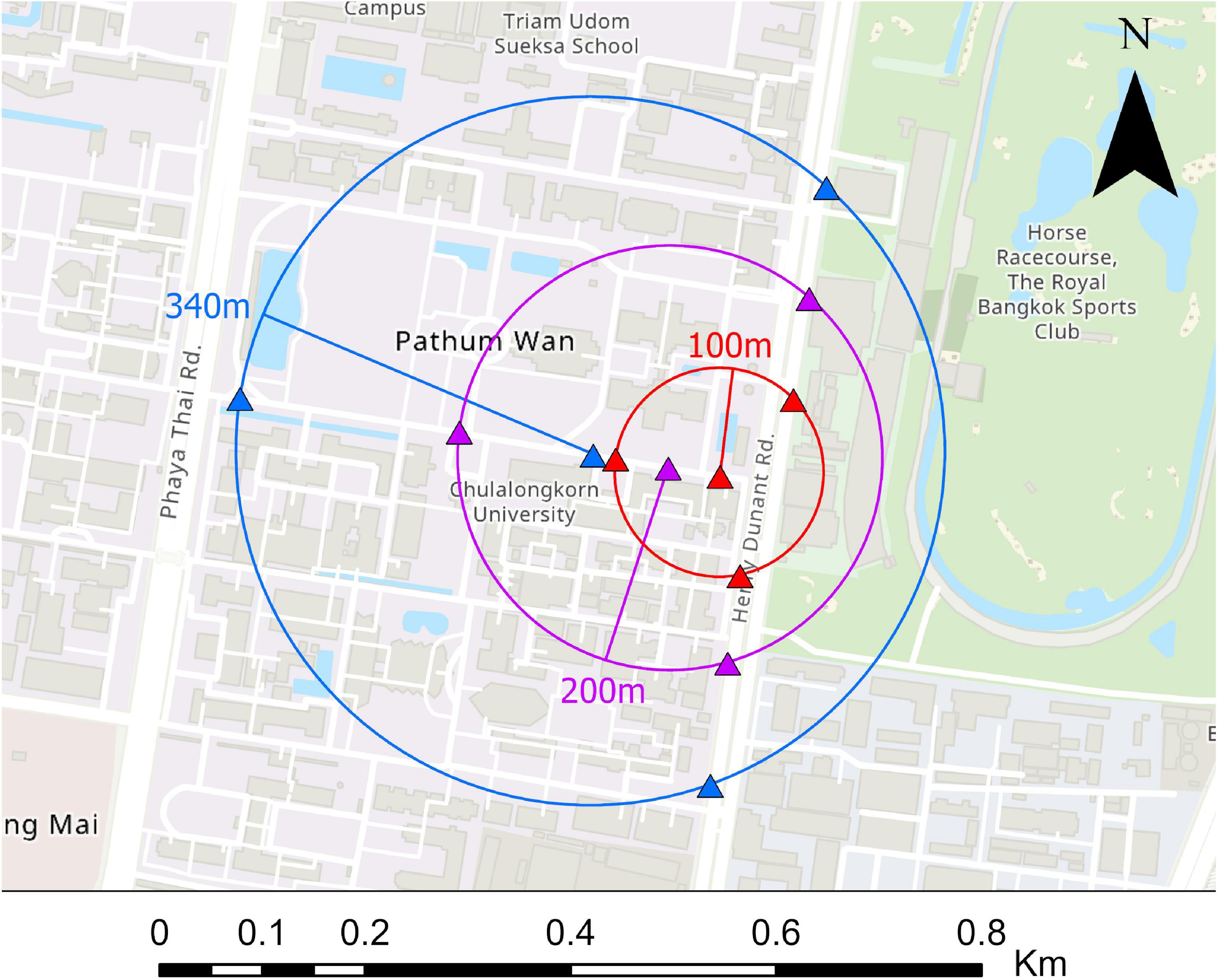
Figure 4. The geometry of the JU410 arrays at site CU; triangles represent the JU410 sensors.

For the 3-, 5-, and 10-m arrays in all five sites, four sets of HS-1 sensors were used with the data logger (Figure 5A). HS-1 is a single-channel seismograph that records vertical velocity. The data was recorded for at least 15 min at a sampling frequency of 100 Hz. For the arrays of 50-m radius or larger, JU410 were used at a sampling frequency of 200 Hz (Figure 5B). JU410 is a data acquisition system with an integrated sensor, data logger and internal GPS. The sensor is a 3-axis servo type accelerograph developed by Japan Aviation Electronics Industry, Ltd., JU410 records data along two perpendicular horizontal channels and one vertical channel. Each dataset by JU410 was recorded for a minimum of 40 min.

FIGURE 5

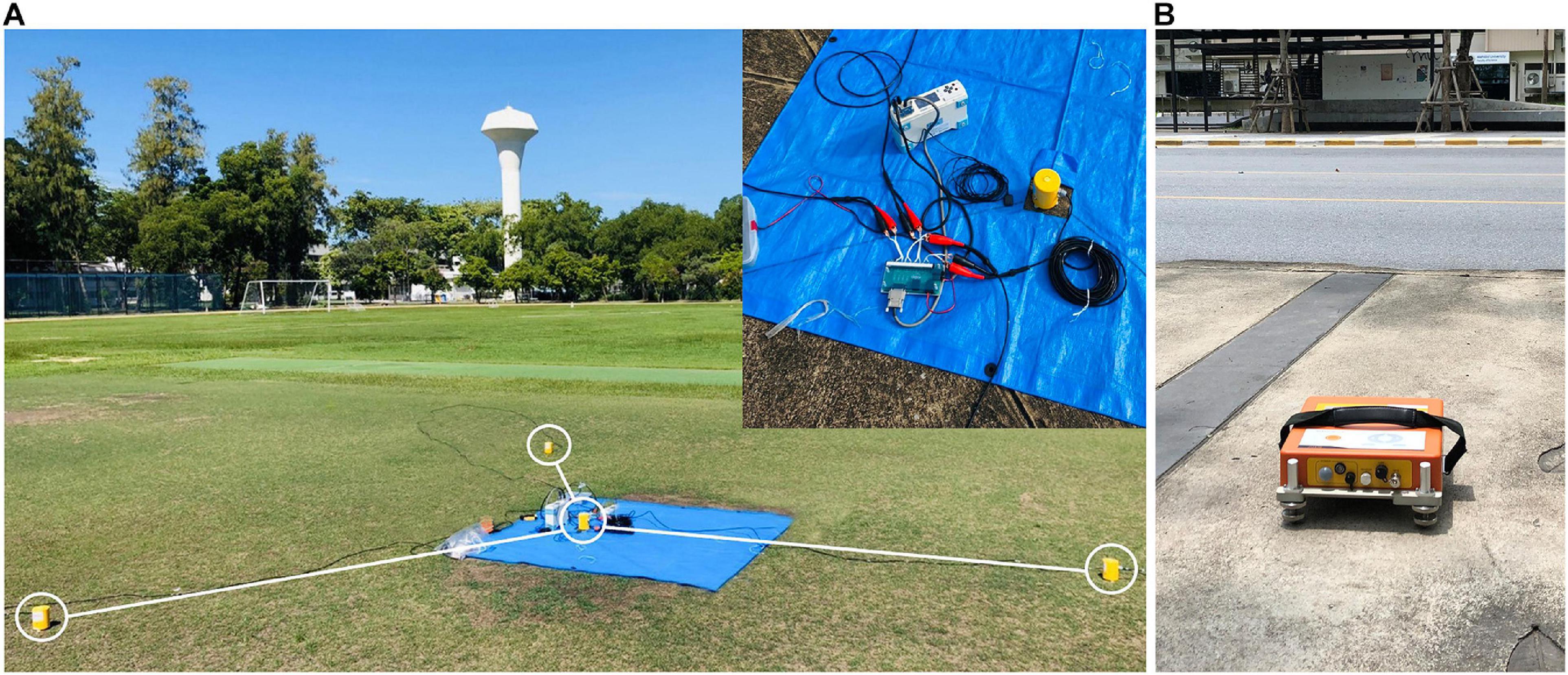
Figure 5. (A) Velocity-meter (Data logger HKS-9700 with HS-1 sensor) being used for small aperture array measurement in Bangkok (B) Datamark JU410 recording data at site MU.

Microtremor Data Analysis

Horizontal-to-Vertical Spectrum Ratio Analysis

The horizontal-to-vertical spectrum ratio (HVSR) of a single point measurement in three directions can be used to find the fundamental frequency of a site. This method was proposed by Nogoshi and Igarashi (1970) and was further developed and made widespread by Nakamura (1989). The HVSR analysis is a robust and low-cost technique to estimate the soil fundamental frequency. However, to estimate the amplification or bandwidth for the amplification, earthquake recordings need to be used as well (Bard, 1999). Here we calculated HVSR using:

$$H/V\left(\mathrm{\omega }\right)=\frac{\sqrt{F_{NS}{(\mathrm{\omega })}^2+F_{EW}{(\mathrm{\omega })}^2}}{F_{UD}(\mathrm{\omega })}(1)$$

Where, F_NS(ω), F_EW(ω), and F_UD(ω) are the Fourier amplitude spectra in the north–south, east–west, and up–down directions, respectively. The H/V(ω) spectrum resembles the transfer ratio and the peak corresponds to the fundamental frequency of the site (Nakamura, 1989). Equation (1) was applied to obtain the H/V spectrum; then, the frequency corresponding to the peak was noted as the predominant ground frequency.

The accuracy of the results obtained from the JU410 records was verified by using another monitoring instrument. The sensor HS-1 3-Component Mini SeisMonitor by Geospace Technologies was used with a data logger HKS-9700. The sensor has three HS-1 seismometers with a natural frequency of 2.0 Hz, orthogonally arranged in two horizontal directions and one vertical. The sensor is especially designed for three-component low-frequency monitoring with a wide operating temperature range of −40°C to 100°C (Geospace Technologies, 2020). The site used for the comparison is the deepest part of the Kyoto basin located at Nishikamosu Makishimacho, Uji, Kyoto, Japan (34.91°N, 135.77°E) (red triangle in map, Figure 6; Kiyono et al., 2001). The depth of the sedimentary basin above the bedrock is 800 m at the recording site (Kansai Geo-informatics Agency, 2002). The site is far from traffic, urban or industrial noises. Recordings, each 15 min long, were carried out twice by two instruments simultaneously. Figure 6 shows the results of the HVSR analysis. The curves overlay each other in all the frequency ranges above 0.3 Hz; below 0.3 Hz the JU420 result drifts upward. Both instruments were able to capture the predominant ground frequency reliably in the low-frequency range at around 0.3–0.4 Hz. The JU410 user manual states that it’s operating range as 0–40°C (Hakusan Corporation, 2015). The temperature during the recording site at Bangkok and Kyoto was mostly 36°C which is close to the upper range. This might be the reason for the variation of the results in frequencies below 0.3 Hz. Thus, the HVSR results of records in Bangkok are validated in the frequency range of 0.3–10 Hz.

FIGURE 6

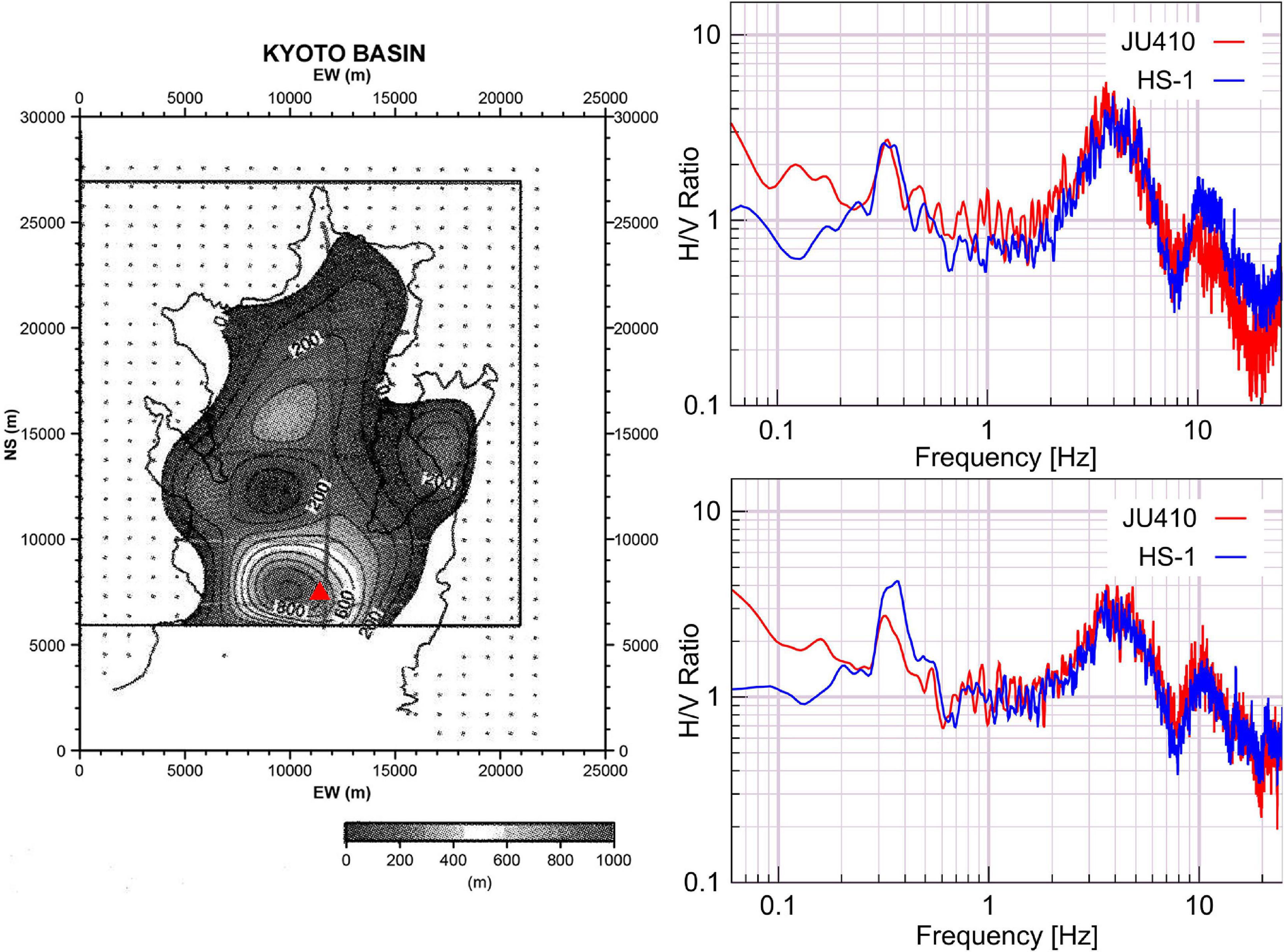
Figure 6. Left: Basin depth of the site used for the comparison inside Kyoto basin (after Kiyono et al., 2001). Right: Comparison of HVSR from two sets of data recorded with JU410 and sensor HS-1 simultaneously.

From the three sets of 4-point array data recorded by JU410, there are 12 single point measurements at AIT, CU, KU, and MU. All the JU410 records were used to calculate the HVSR. At each site, the red curves are the HVSR results from the multiple single point recordings (Figure 7), from 0.3 to 10 Hz. The mean and mean ± one standard deviation were calculated and are plotted in black. There is a clear peak at 0.76 s at AIT, 0.79 s at CU, 0.68 s at KU, 0.86 s at MU, and 0.85 s at TMD. The fundamental resonant time period of the ground at the low-frequency range is not clear. Papadopoulos et al. (2017) compared the HVSR of earthquake records (HVSRE) with HVSR of ambient vibration recorded with a speedometer for the frequency band of 0.2–20 Hz. The methods showed good agreement for the lower and higher predominant frequency depending on two main seismic discontinuities for all the sites except the ones near the edge of the basin. The amplitude for HVSRE was slightly higher than that of HVSR. For accurate estimation of lower predominant frequency in our study area, sensors with higher corner period need to be used for ambient vibration recordings.

FIGURE 7

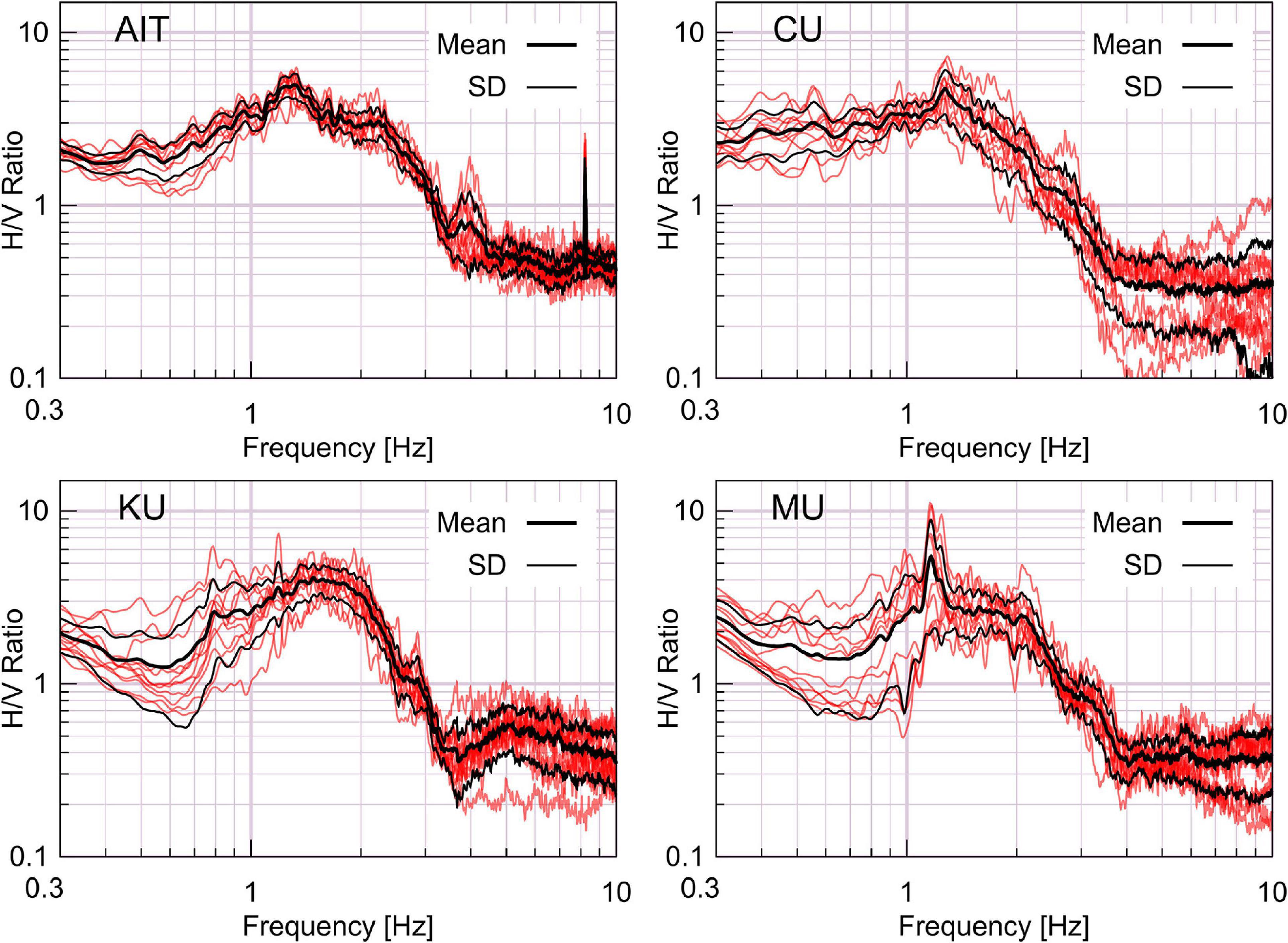
Figure 7. H/V spectra at four survey sites. At each site, the red lines are the H/V ratios from multiple single-point recordings. Mean and mean ± one standard deviation are plotted with black lines.

Methods for Array Analysis

To obtain the dispersion curve of the Rayleigh-wave phase velocity from the array recordings, the Spatial Autocorrelation method (SPAC method) and Centerless Circular Array method (CCA method) were used. These methods are discussed briefly in the following sections.

The SPAC Method

The SPAC method (Aki, 1957) is widely used to deduce the phase velocities of surface waves from microtremor recordings. A station at the center of the array is mandatory for this method. Simultaneous recordings from at least three stations are required; however, a four-station geometry with three equidistant stations along the circumference is generally used. A detailed explanation of the principal of detection of Love and Rayleigh waves from the vertical component microtremor and estimation of the phase velocity and subsurface structure by the SPAC-method can be found in Okada (2003). Estrella and Gonzalez (2003) shows the process for obtaining the Rayleigh-wave dispersion curve by the SPAC method in brief as follows.

If the microtremors are the harmonic waves with frequency ω, the velocity waveforms are represented as u(0,0,ω,t) at the center of the array C(0,0) and u(r,θ,ω,t) at point X(r,θ) along the circumference. The spatial autocorrelation (SPAC) function is

$$\mathrm{\varphi }(r,\mathrm{\theta },\mathrm{\omega })=\overline{u(0,0,\mathrm{\omega },t).u(r,\mathrm{\theta },\mathrm{\omega },t)}(2)$$

Where, $\overline{u\left(t\right)}$ is the average velocity of the wave in the time domain. The SPAC coefficient ρ is the average of the SPAC function ϕ in all directions in the circular array, described as:

$$\mathrm{\rho }(\text{r},\mathrm{\omega })=\frac{1}{2\mathrm{\pi }.\mathrm{\varphi }(0,\mathrm{\omega })}\underset{0}{\overset{2\mathrm{\pi }}{\int }}\mathrm{\varphi }(r,\mathrm{\theta },\mathrm{\omega })d\mathrm{\theta }(3)$$

Where, ϕ(0,ω) is the SPAC function at the center of the array C(0,0). Integrating Equation (3) gives,

$$\mathrm{\rho }(\text{r},\mathrm{\omega })=J_0\left(\frac{\mathrm{\omega }r}{c(\mathrm{\omega })}\right)(4)$$

Where, J₀ is the Bessel function of the first kind of order zero and c(ω) is the phase velocity at frequency ω. ρ(r,ω) is obtained from recorded microtremors as:

$$\mathrm{\rho }(\text{r},\mathrm{\omega })=\frac{1}{2\mathrm{\pi }}\underset{0}{\overset{2\mathrm{\pi }}{\int }}\frac{Re[S_{CX}(\mathrm{\omega },r,\mathrm{\theta })]}{\sqrt{S_C(\mathrm{\omega }).S_X(\mathrm{\omega },r,\mathrm{\theta })}}d\mathrm{\theta }(5)$$

Where, S_C(ω) and S_X(ω,r,θ) are the power spectral densities of the microtremors at sites C and X, respectively, and S_CX(ω,r,θ) is the cross-spectrum of the recordings at sites C and X. When ρ(r,ω) is known, the phase velocity for every frequency can be obtained from Equation (4).

The CCA Method

This is a relatively new method, introduced by Cho et al. (2004). This method assumes that the Rayleigh- and Love-wave components are uncorrelated and can be taken as random field stationary in time and space. The noise present in the signal is regarded as stationary, uncorrelated with the signal, mutually incoherent and identical in intensity in the different sensor records. The process of the CCA method is outlined in the following sections (Cho et al., 2006).

For a circular array of radius r, Z(t,r,θ) is the vertical component of the microtremors. When the seismograms are integrated with respect to azimuth, two complex waveforms are obtained:

$$Z_0(\text{t},\text{r})=\underset{-\mathrm{\pi }}{\overset{\mathrm{\pi }}{\int }}Z(t,r,\mathrm{\theta })d\mathrm{\theta }(6)$$

$$Z_1(\text{t},\text{r})=\underset{-\mathrm{\pi }}{\overset{\mathrm{\pi }}{\int }}Z(t,r,\mathrm{\theta })\exp \left(i\mathrm{\theta }\right)d\mathrm{\theta }(7)$$

The power spectral densities of Equations (6) and (7) can be presented as:

$$G_{Z0Z0}(\text{r},\text{r},\mathrm{\omega })=4{\mathrm{\pi }}^2\sum _{i=1}^{M^R}{f}_i^{RV}\left(w\right)J_0^2(r{k}_i^R\left(\mathrm{\omega }\right))(8)$$

$$G_{Z1Z1}(\text{r},\text{r},\mathrm{\omega })=4{\mathrm{\pi }}^2\sum _{i=1}^{M^R}{f}_i^{RV}\left(\mathrm{\omega }\right)J_1^2(r{k}_i^R\left(\mathrm{\omega }\right))(9)$$

Where, ω is the angular frequency, M^R is the number of Rayleigh-wave modes, $f_i^{RV}(\mathrm{\omega })$ is the intensity of the vertical component of the i^th mode Rayleigh waves, J₀(.) and J₁(.) are the zero- and first-order Bessel functions of the first kind, and $k_i^R\left(\mathrm{\omega }\right)$ is the wavenumber of the i^th mode Rayleigh wave. Taking the ratio of Equations (8) and (9) and assuming the dominance of the fundamental mode, the ratio reduces to:

$$\frac{G_{Z0Z0}(\text{r},\text{r},\mathrm{\omega })}{G_{Z1Z1}(\text{r},\text{r},\mathrm{\omega })}=\frac{J_0^2(r{k}^R\left(\mathrm{\omega }\right))}{J_1^2(r{k}^R\left(\mathrm{\omega }\right))}(10)$$

Where, k^R (ω) is the phase velocity of the fundamental-mode Rayleigh waves. When the left-hand side of Equation (10) is known from recordings, rk^R can be estimated for each frequency ω. Since r is known, the wavenumber is known and can be used to calculate the phase velocity. Equation (10) is applied in noise-free conditions. When noise is present in the signal, Equation (11) should be used to avoid underestimating the phase velocity at the low-frequency range.

$$\frac{G_{Z0Z0}(\text{r},\text{r},\mathrm{\omega })}{G_{Z1Z1}(\text{r},\text{r},\mathrm{\omega })}=\frac{J_0^2\left(r{k}^R\left(\mathrm{\omega }\right)\right)+{\mathrm{\epsilon }}^v(\mathrm{\omega })/N}{J_1^2(r{k}^R\left(\mathrm{\omega }\right))+{\mathrm{\epsilon }}^v(\mathrm{\omega })/N}(11)$$

Where, N is the number of sensors along the circle and ε^v(ω) is the noise to signal ratio.

Analysis of Array Records

Comparing the results of the SPAC method and CCA method for the analysis of the Osaka Basin data, the CCA method analyzed more than double the length of wavelength compared with the SPAC method for array radius up to 50 m. For arrays with radiuses of more than 100 m, both methods had the same level of analysis capability (Yoshimi, 2012). In our analysis, the CCA method was able to analyze longer wavelengths for the arrays with radiuses of 3, 5, and 10 m in all the sites, as reported. Therefore, for all the data of the 3-, 5-, and 10-m arrays, the CCA method was used. For the data of the larger arrays, analysis by both methods was carried out. Although both methods produced similar peak locations and dispersion curves for the three larger arrays, in sites CU, KU, and MU, the SPAC method gave clearer peaks in the individual dispersion curve whereas for site AIT, the results from CCA method were clearer. Accordingly, the SPAC or CCA method was chosen to derive the observed dispersion curves.

Figure 8 shows the dispersion curves for the five sites with different colors for the various array sizes. The inversion was done by conventional forward modeling. During the inversion, the P-wave velocity (V_p) and density (ρ) were required as well as V_s, V_p, and ρ were calculated by using the following empirical equations from Ludwig et al. (1970).

FIGURE 8

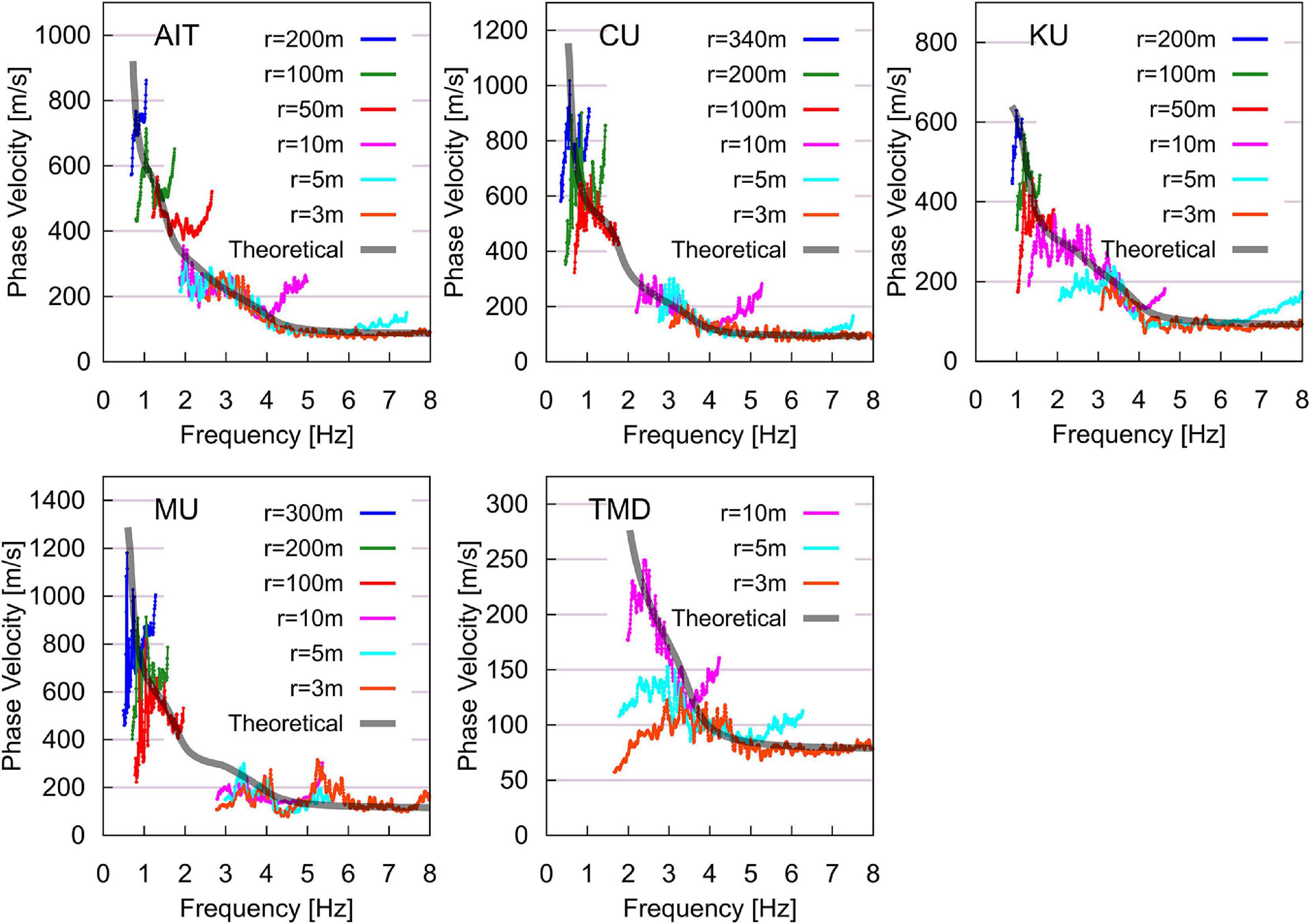
Figure 8. Phase-velocity dispersion curves of the Rayleigh waves at five sites. The gray lines were derived from the final inversion profile; the colored lines represent the various array sizes.

$$V_p\left(km/s\right)=0.9409+2.0947V_s-0.8206V_s^2+0.2683V_s^3$$

$$-0.0251V_s^4(12)$$

$$\mathrm{\rho }\left(gm/c{m}^3\right)=1.6612V_p-0.4721V_p^2+0.0671V_p^3$$

$$-0.0043V_p^4+0.000106V_p^5(13)$$

The phase-velocity dispersion curves calculated from the microtremor data (colored lines) and the theoretical dispersion curve calculated from final inversion profile (gray curve) display a good fit.

The deepest velocity profiles were obtained in sites CU and MU (Table 2 and Figure 9). The largest array diameter used at CU was 340 m and at MU it was 300 m whereas in KU and AIT, the 200-m array was the largest. In TMD, the inversion was performed down to the layer with Vs = 330 m/s above the layer with Vs = 650 m/s due to the small array radius (up to 10 m) at that site.

TABLE 2

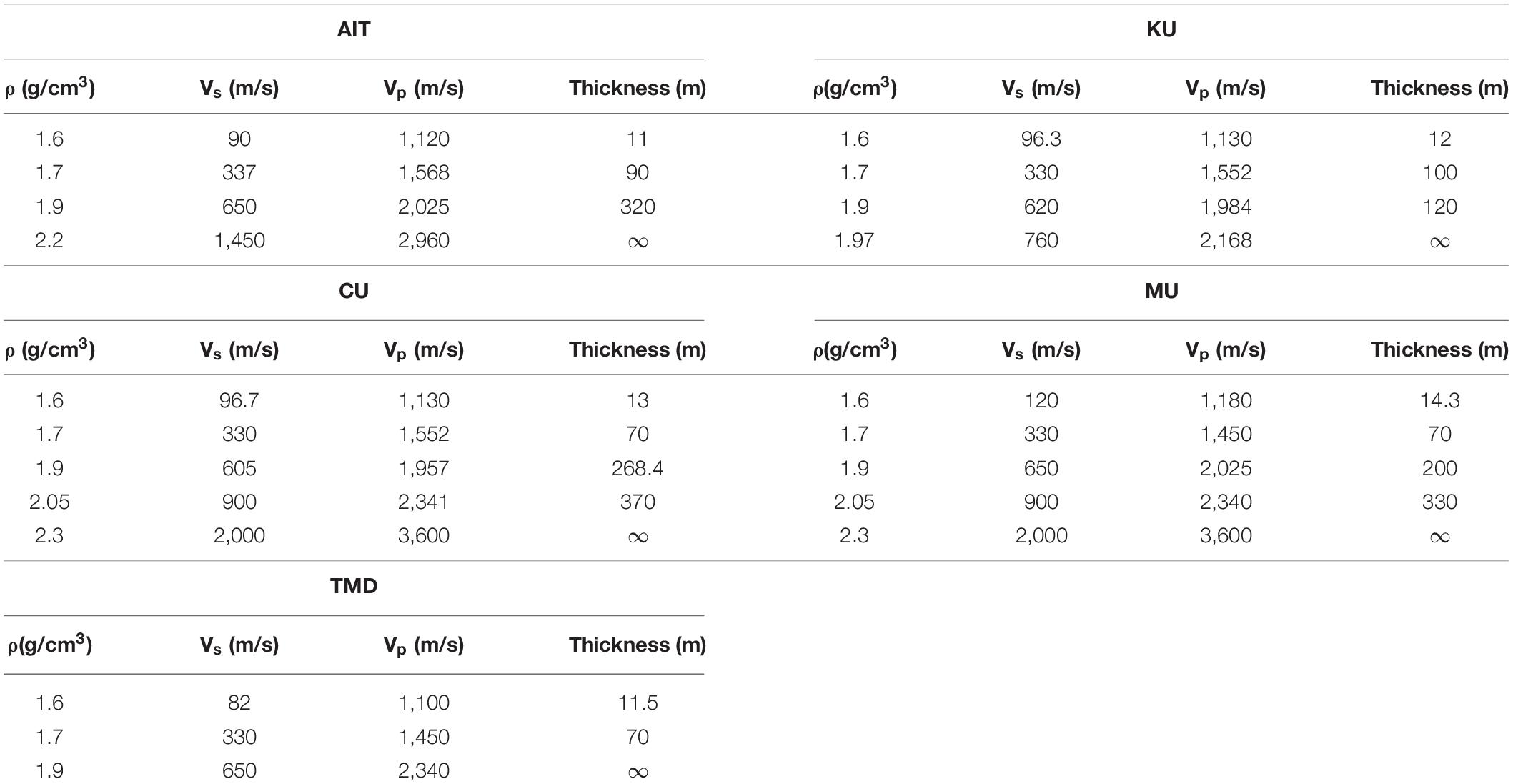
Table 2. Velocity profiles from the inversion of the dispersion curves shown in Figure 8.

FIGURE 9

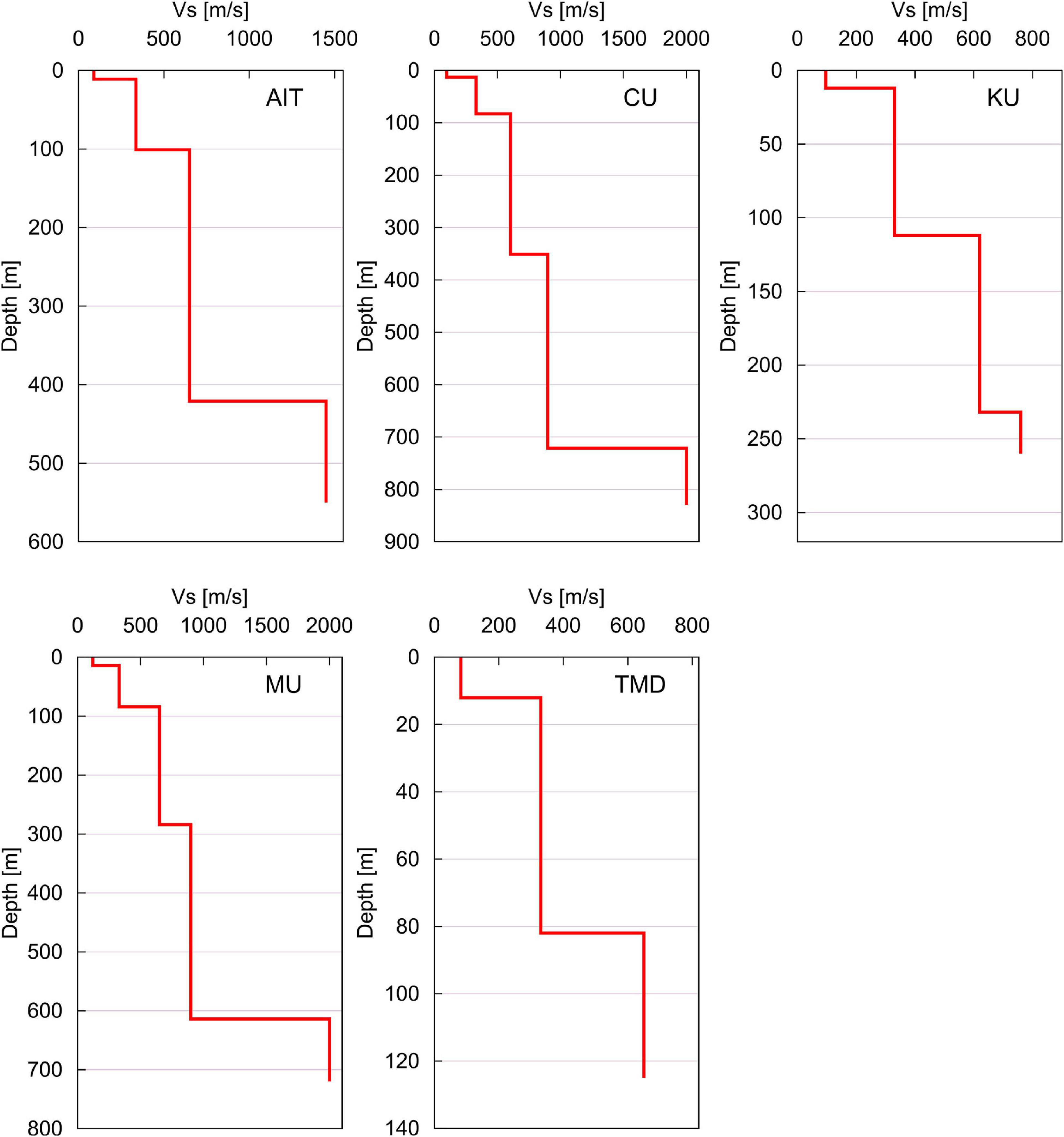
Figure 9. Velocity profiles from inversion of the dispersion curves shown in Figure 8.

The results show that Vs of the top clay layer is 82–120 m/s. The depth of this soft clay is 11–14.3 m. Such low Vs values for the top-most clay layer have been reported by various researchers. The top layer of soft clay (12–16 m deep) is highly compressible (Phien-wej et al., 2006); because of this soft clay layer, buildings in Bangkok need pile foundations and even small buildings have piles driven to depths of 6–12 m.

The Vs depth profiles at the recording sites along the N–S and E–W lines (Figure 3) were plotted using the inversion results and are shown in Figure 10. Along the N–S, the depth of the third layer, with Vs = 605–650 m/s, is less at KU than at AIT and CU, which implies that the northern and southern parts of the basin are deeper than the center. Along the E–W line, the third layer, with Vs = 605–650 m/s, is deeper at CU than at MU. This implies that the basin is deeper near CU and the depth decreases northward near KU and westward near MU.

FIGURE 10

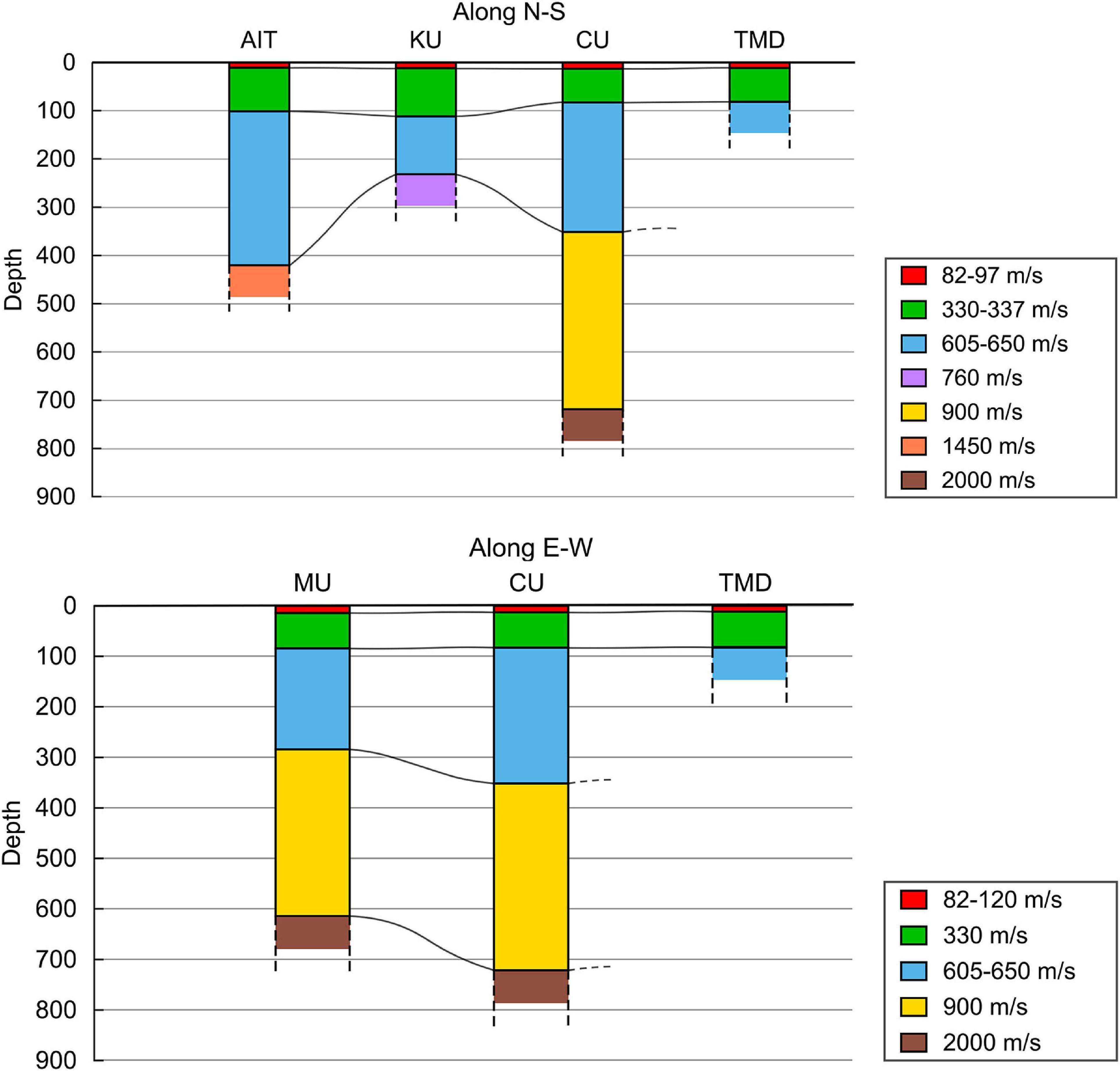
Figure 10. S-wave velocity profiles along the N–S and E–W lines shown in Figure 3.

The 1-D transfer functions derived from the multiple reflection analysis of the inverted profiles for all the sites except TMD are shown in Figure 11. The predominant frequencies at the four sites are similar at around 2 Hz and all show higher amplitudes from 0.3 to 2 Hz. A detailed comparison was performed with the records observed at TMD (Figure 12). The distance between the strong-motion stations TMD and SRDT is 179 km (see Figure 1). SRDT is located at a rocky site whereas TMD is in the sediment of the Bangkok basin. The ratio of the TMD and SRDT HVSRs of the seismic waves recorded in the 2008 Sichuan Earthquake was used to find the site-effect of the basin (Figure 12A). The plot of this ratio is shown alongside with HVSR of the single-point three-direction microtremor measurement by JU410 at TMD (Figure 12B) and 1-D transfer function obtained from the inversion model at the site (Figure 12C).

FIGURE 11

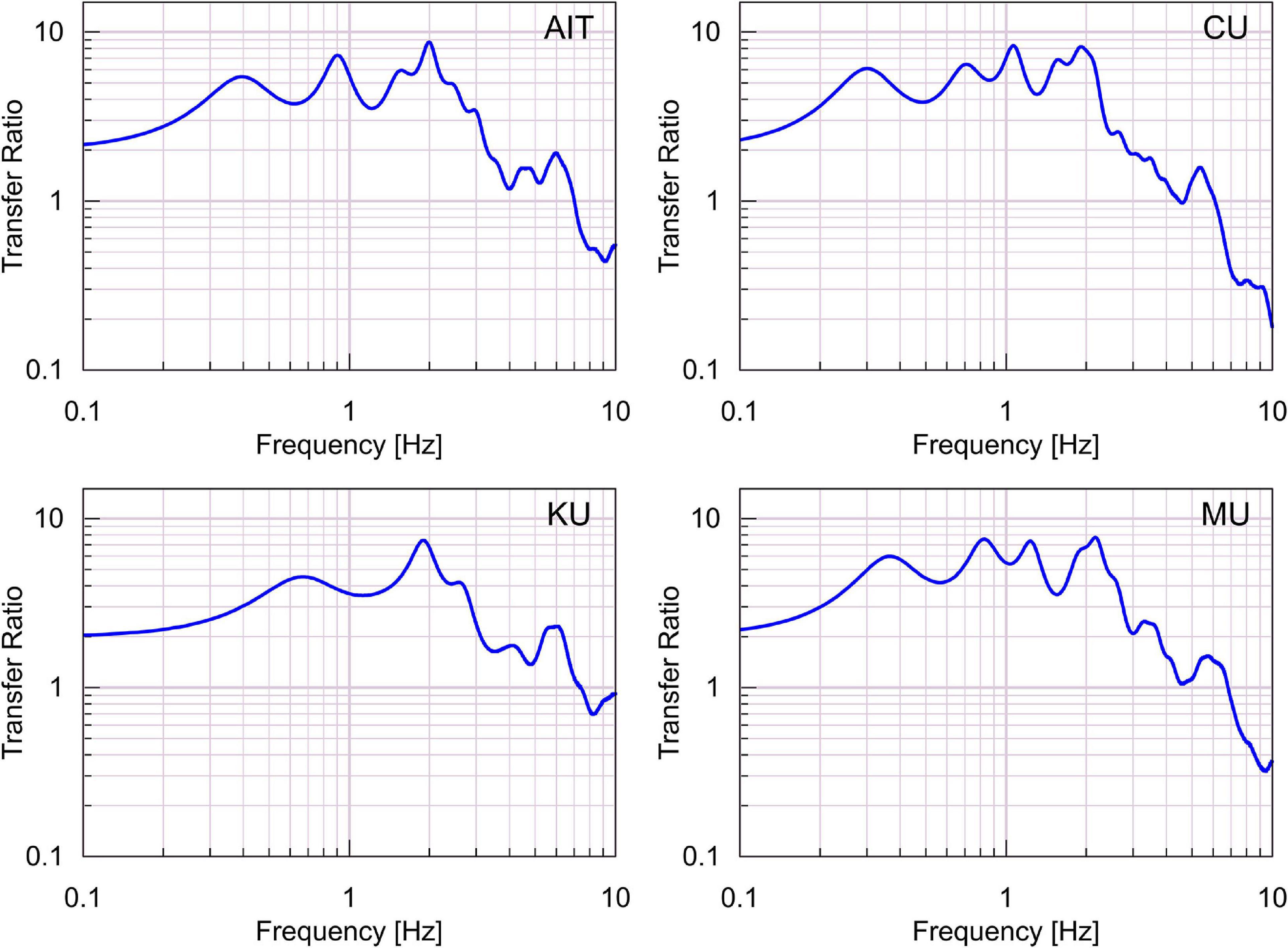
Figure 11. 1-D linear transfer function from the multiple reflection analysis of the inverted models.

FIGURE 12

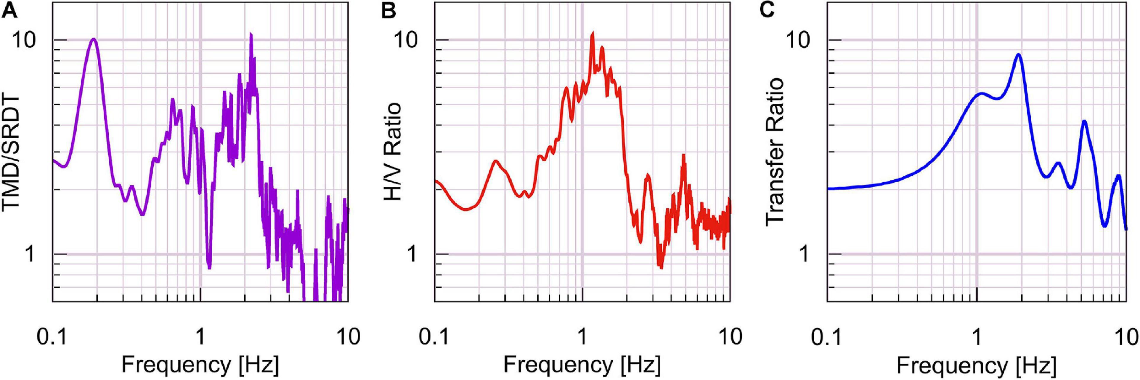
Figure 12. (A) Ratio of HVSR of earthquake records at TMD and SRDT, (B) HVSR of single-point microtremor measurement at TMD, (C) 1-D transfer function from the inversion model at TMD.

The peak and shape of the HVSR and transfer function are in good agreement, with a peak frequency of 1–2 Hz. However, another low-frequency peak appears in Figure 12A. As mentioned earlier, the array radius in TMD is small, therefore we cannot investigate the deeper layer information that appears in Figure 12C. The 0.2-Hz peak in Figure 12A indicates the existence of deep bedrock. To clarify the long-period HVSR peak, seismometers reliable in low-frequency should be used for further study. Moreover, large-aperture array observations and deep borehole data should be used to establish the deep boundary reliably to estimate the amplification of long-period earthquake waves in Bangkok.

Conclusion

Bangkok lies in soft alluvial deposits in a deep basin; these conditions amplify long-period seismic waves. The HVSR of seismic waves recorded inside the Bangkok basin shows a low-frequency peak at around 5 s. This study presents the microtremor survey technique used in a preliminary geophysical investigation at five sites in Bangkok. We conducted single-point and array recordings and HVSR analysis of single-point ambient vibration recordings. The accuracy of the accelerometer used for the ambient data recording was verified in the frequency range of 0.3–10 Hz by comparing with velocity-meter results. Thus, the HVSR spectra of the sites in Bangkok were verified in that range. The estimated predominant period was long—in the range of 0.68–0.86 s. A predominant period longer than 2 s was not identified. From the array records, the dispersion curves of the Rayleigh-wave phase velocity were extracted using the SPAC and CCA methods. The inversion was performed and the Vs depth profiles were plotted. The results show that Vs of the top clay layer is low: 82–120 m/s at depths of 11–14.3 m. The basin is deeper near CU and the depth decreases northward near KU and westward near MU. The 1-D transfer functions derived by multiple reflection analysis of the inversion profiles for the four sites show the predominant frequencies at around 2 Hz and higher amplitudes from 0.3 to 2 Hz. For the site TMD, the ratio of the TMD to SRDT HVSRs of the seismic waves recorded in the 2008 Sichuan Earthquake, the HVSR of the single-point three-direction microtremor measurement and the 1-D transfer function obtained from the inversion model show good agreement.

The low-frequency peak in the HVSR of the earthquakes and the existence of sediment with low Vs implies that Bangkok is at risk of amplification of long-period earthquake waves. To clarify the deep bedrock boundary, large-aperture array observations, seismometers reliable in low-frequency and/or deep borehole data should be used for further study.

Data Availability Statement

The original contributions presented in the study are included in the article. Requests to access the bulk datasets analyzed in this study should be directed to the corresponding author, BS (subedi.bidhya.24s@st.kyoto-u.ac.jp).

Author Contributions

BS performed analysis of the earthquake records and microtremor records, prepared figures, and wrote the manuscript. JK conceptualized the study, supervised the data recording, processing, and manuscript preparation. AF supervised the data processing. TO collected the earthquake records in Bangkok. All the authors performed the microtremor survey in Bangkok, Thailand, and contributed to the discussions. BS and JK carried out the microtremor observations in Kyoto basin. All the authors contributed to the article and approved the submitted version.

Funding

This work was supported by the project “International Collaborative Research on Long-period Earthquake Early Warning for Bangkok Metropolitan Area.” The project was supported by the Supporting Program for Interaction-Based Initiative Team Studies (SPIRITS) funded by Kyoto University.

Conflict of Interest

The authors declare that the research was conducted in the absence of any commercial or financial relationships that could be construed as a potential conflict of interest.

Acknowledgments

We are grateful to the people of Bangkok for the kind support and cooperation during the microtremor survey.

References

Aki, K. (1957). Space and time spectra of stationary stochastic waves, with special reference to microtremors. Bull. Earthq. Res. Inst. Univ. Tokyo 35, 415–457.

Google Scholar

Baoqi, C., and Renfa, C. (1990). The srinakarin reservoir earthquake, Thailand. J. Southeast Asian Earth Sci. 4, 49–54. doi: 10.1016/0743-9547(90)90024-8

CrossRef Full Text | Google Scholar

Bard, P. Y. (1999). “Microtremors measurements: a tool for site effect estimation?,” in Proceedings of the Second International Symposium on the The Effects of Surface Geology on Seismic Motion, Vol. 3, eds K. Irikura, K. Kudo, H. Okada, and T. Sasatani (Rotterdam: Balkema), 1251–1279.

Google Scholar

Cho, I., Tada, T., and Shinozaki, Y. (2004). A new method to determine phase velocities of Rayleigh waves from microseisms. Geophysics 69, 1535–1551. doi: 10.1190/1.1836827

CrossRef Full Text | Google Scholar

Cho, I., Tada, T., and Shinozaki, Y. (2006). Centerless circular array method: inferring phase velocities of Rayleigh waves in broad wavelength ranges using microtremor records. J. Geophys. Res. 111:B09315. doi: 10.1029/2005JB004235

CrossRef Full Text | Google Scholar

City Population (2019). Available online at: https://www.citypopulation.de/en/thailand/prov/admin/ (accessed on December 25, 2020).

Google Scholar

DMR (Department of Mineral Resources) (2006). Active Fault Zones in Thailand. Available online at: http://www.dmr.go.th/main.php?filename=fault_En (accessed on October 29, 2020).

Google Scholar

Estrella, H. F., and Gonzalez, J. A. (2003). SPAC: an alternative method to estimate earthquake site effects in mexico city. Geofísica Int. 42, 227–236.

Google Scholar

Geospace Technologies (2020). HS-1 3 Component Array Product Brochure. Available online at: https://www.geospace.com/sensors/hs-1-3-component-array-mini-seismonitor/ (accessed on October 29, 2020).

Google Scholar

Hakusan Corporation (2015). DATAMARK Microtremormeter JU410 User’s Manual, 2nd Edn. Tokyo: HAKUSAN Corporation.

Google Scholar

Kansai Geo-informatics Agency (2002). Shin-Kansai Jiban, Kyoto basin. Osaka: Kansai Geo-informatics Agency, 164. (in Japanese)

Google Scholar

Kiyono, J., Toki, K., and Sakai, Y. (2001). “Ground profile and seismic ground motion of kyoto basin,” in Proceedings of the JSCE Earthquake Engineering Symposium, Vol. 26, 281–284. (in Japanese)

Google Scholar

Ludwig, W. J., Nafe, J. E., and Drake, C. L. (1970). in Seismic Refraction, the Sea 4, ed. A. Maxwell (New York, NY: Wiley Inter Science), 53–84.

Google Scholar

Lukkunaprasit, P. (1993). “State of seismic risk mitigation in Thailand,” in Proceedings of the WSSI Workshop on Seismic Risk Management for Countries of the Asia Pacific Region, Bangkok. doi: 10.1007/978-94-010-0806-8_4

CrossRef Full Text | Google Scholar

Nakamura, Y. (1989). A method for dynamic characteristics estimation of subsurface using microtremor on the ground surface. Q. Rep. Railway Tech. Res. Inst. (RTRI) 30, 25–30.

Google Scholar

Nogoshi, M., and Igarashi, T. (1970). On the propagation characteristics of microtremors. J. Seism. Soc. Jpan. 23, 264–280.

Google Scholar

Okada, H. (2003). The Microtremor Survey Method: Geophysical Monograph Series, no. 12, Society of Exploration Geophysicists. Tulsa, OK: Society Of Exploration Geophysicists.

Google Scholar

Ornthammarath, T. (2013). A note on the strong ground motion recorded during the Mw 6.8 earthquake in Myanmar on 24 March 2011. Bull. Earthq. Eng 11, 241–254. doi: 10.1007/s10518-012-9385-4

CrossRef Full Text | Google Scholar

Ornthammarath, T., and Warnitchai, P. (2016). 5 May 2014 MW 6.1 Mae Lao (Northern Thailand) earthquake: interpretations of recorded ground motion and structural damage”. Earthq. Spectra 32, 1209–1238. doi: 10.1193/081814eqs129m

CrossRef Full Text | Google Scholar

Ornthammarath, T., Warnitchai, P., Worakanchana, K., Zaman, S., Ragnar, S., and Lai, C. G. (2010). Probabilistic seismic hazard assessment for Thailand. Bull. Earthq. Eng. 9, 367–394. doi: 10.1007/s10518-010-9197-3

CrossRef Full Text | Google Scholar

Pananont, P., Wechbunthung, B., Putthapiban, P., and Wattanadilokkul, D. (2011). Seismic activities in Kanchanaburi: past and present. Songkhlanakarin J. Sci. Technol. 33A, 355-364.

Google Scholar

Papadopoulos, I., Papazachos, C., Savvaidis, A., Theodoulidis, N., and Vallianatos, F. (2017). Seismic microzonation of the broader Chania basin area (Southern Greece) from the joint evaluation of ambient noise and earthquake recordings. Bull. Earthq. Eng. 15, 861–888. doi: 10.1007/s10518-016-0019-0

CrossRef Full Text | Google Scholar

Phien-wej, N., Giao, P. H., and Nutalaya, P. (2006). Land subsidence in Bangkok Thailand. Eng. Geol. 82, 187–201. doi: 10.1016/j.enggeo.2005.10.004

CrossRef Full Text | Google Scholar

Sinsakul, S. (2000). Late quaternary geology of the lower central plain Thailand. J. Asian Earth Sci. 18, 415–426. doi: 10.1016/s1367-9120(99)00075-9

CrossRef Full Text | Google Scholar

Yoshimi, M. (2012). Resolution of the SPAC, CCA, nc-CCA, and V-method for microtremor array survey on deep sedimentary basin—case of the Osaka basin. J. Jpn. Soc. Civil Eng. A1 (Struct. Eng. Earthq. Eng.) 68, I_220–I_226.

Google Scholar