Encoding Time-Series Ground Motions as Images for Convolutional Neural Networks-Based Seismic Damage Evaluation

Introduction

Traditional seismic fragility curves based on a scalar intensity measure (IM) have been widely used to generate fragility estimates in earthquake events (Hwang et al., 2001; Baker and Cornell, 2005; Cimellaro et al., 2010; Xu et al., 2020a). Although they are affected by geometry and material uncertainties, seismic fragility estimates are dominated by the earthquake uncertainty (Kwon and Elnashai, 2006; Padgett and DesRoches, 2007; Jalayer et al., 2014; Mangalathu et al., 2018; Xie et al., 2020). The traditional seismic fragility curves using one IM to propagate the primary earthquake uncertainty have several disadvantages. First, the fragility curves generated from a single IM are likely inaccurate because of the weak dependence of seismic structural responses on the selected IM (Grigoriu, 2016). Second, different ground motions at the same IM level generate the same fragility estimates, thus overlooking their record-to-record variation. To address the first disadvantage, an optimal IM that can sufficiently characterize ground motions is recommended in seismic fragility analysis (Padgett et al., 2008). However, previous studies of correlation between IMs and structural damage indices showed that the optimal IM varies with the dynamic structural properties and the used damage index (Riddell, 2007; Kostinakis et al., 2015). It is a daunting assignment to find the optimal IM from dozens, if not hundreds, of existing IMs when generating the traditional fragility curves. To address the second disadvantage, researchers built a desired confidence interval confined with the pre-determined upper and lower bounds around the traditional fragility curves (e.g., Jalayer et al., 2017; Miano et al., 2018; Wang et al., 2018). Thus, the confidence interval corresponds to a range of fragilities at a certain IM level, which can account for the record-to-record variation to some degree. An alternative approach involved the use of multiple IMs. For example, Baker and Cornell (2005) used two IMs to better characterize the ground motions in fragility estimates. Morfidis and Kostinakis (2018, 2019) investigated the ability of multilayer feedforward perceptron networks (MFP) and radial-basis function networks (RBF) to predict the reinforced concrete (r/c) buildings’ seismic damage state with 14 IMs as input. They concluded that both MFP and RBF neural networks could reliably and rapidly predict the damage states of r/c buildings based on the case study results of 30 r/c buildings. Du et al. (2020) used five IMs to facilitate more accurate and reliable regional seismic risk estimates. Xu et al. (2020b) included up to 48 IMs as input to machine learning models to predict the structural damage states of different types of buildings. They used an iterative approach to filter the optimal IMs from different combinations of IM candidates by training the machine learning models multiple times. Overall, the traditional seismic damage evaluation requires time-consuming manual computations and the selection of optimal IMs from a large pool of IM candidates in order to represent the ground motion record-to-record variation and achieve the best performance in damage evaluation.

Since real-time seismogram data can be obtained from an advanced system such as the ShakeMap (Wald et al., 2006) at seismograph stations (USGS, 2021), they may be preferably used for an in-situ evaluation of seismic damage through Convolutional Neural Networks (CNNs). To achieve this, the features of the ground motion records need to be automatically extracted as IMs. CNNs are well known for their powerful feature extraction ability and have been widely used in image and video analysis (LeCun et al., 1998, 2010; Kussul et al., 2006; Lecun et al., 2015; Li et al., 2016). In addition, CNNs have been successfully applied to time-series data. For example, Wang and Oates (2015a,b) used Gramian angular summation/difference fields (GAF) and Markov transition fields (MTF) to generate the compound GAF–MTF images of time series for tiled CNN classification. Their approach was demonstrated to yield competitive results for time series classification compared to existing best time-series classification methods. Debayle et al. (2018) proposed to use the recurrence plots (RP) to transform one-dimensional (1D) time series to two-dimensional (2D) texture images for deep CNN classification. Their RP image-based classification approach proved to outperform the traditional classification framework and the new CNN-based classification (GAF–MTF images with CNN). Recently, Mangalathu and Jeon (2020) proposed to use CNNs to rapidly evaluate the damage of structures. They used the wavelet transform (WT) to format 320 ground acceleration records as one-channel images to characterize the temporal and spectral nonlinearity of ground motions. Those images were labeled by their resulting damage states obtained from nonlinear time history analysis (NLTHA), and then inputted into the CNN classifier. The trained CNN classifier was used to predict the damage states caused by future ground motions. The CNN-based approach of ground motion record classification avoids the process of IM selection and computation, and thus is suitable for rapid post-earthquake damage evaluation (Mangalathu and Jeon, 2020).

However, there are still some shortcomings in the current CNN-based classification methods for ground motions. First, there is no agreement on which image encoding technique and its corresponding image size (width × height × channel) is most suitable for ground-motion image encoding. Second, the duration and sampling frequency of ground motions lead to thousands or even tens of thousands of data points in the ground motion records. This can result in very large time-series images and create a difficulty for CNN training. In this study, we propose a new image encoding technique based on time-series segmentation (TS) to transform the acceleration (A), velocity (V), and displacement (D) records of each ground motion event to a three-channel AVD image with a pre-defined size of width × height. We will compare the CNN classification performance trained by the newly proposed TS technique with that of two state-of-the-art time-series image encoding techniques, RP and WT. In addition, these CNN-based seismic evaluation approaches will be compared to the state-of-the-art machine-learning IM-based approach proposed by Xu et al. (2020b). Finally, the most suitable ground-motion AVD image encoding techniques and their corresponding image sizes will be recommended for future studies, based on their classification performance and computational efficiency.

Convolutional Neural Networks-Based Seismic Damage Evaluation Method

A CNN for seismic damage evaluation can be regarded as a classifier of ground motions into different categories according to their resulting damage states to a structure. For example, three damage states, green (ready to occupy), yellow (need detailed inspection before occupying), and red (unsafe to use) as specified in the ATC-40 Guidelines (Applied Technology Council, 1996) were used to label ground motion records in Mangalathu and Jeon (2020). In their case study of a nonductile building frame, the nonlinear response of beam-column joints was selected as the dominant failure mode and the median drift obtained from NLTHA was used to determine the damage labels. If a record caused a maximum drift ratio less than 1.2%, the record was assigned the green label. If a ground motion record caused the maximum drift ratio to be between 1.2 and 2.4%, the record was labeled as the yellow tag. If the maximum drift ratio was beyond 2.4%, the corresponding record was assigned the red tag. These labeled records were transformed into labeled 2D images by WT and used as training samples for the CNN model. Once properly trained using the collected ground-motion images, the CNN classifier would be run in near real time to rapidly predict the damage states of the frame building caused by future ground motions.

Proper image encoding of ground motion records and a good CNN architecture are the two important factors for CNN-based seismic damage evaluation without the use of traditional IMs. Figure 1 shows the framework of this CNN-based methodology for seismic damage evaluation without specified IMs. The CNN seismic classifier is trained using the collected ground-motion images that are labeled by their resulting damage states to a target structure via NLTHA. Thus, the damage state of the target structure caused by a future earthquake event can be predicted by the previously trained CNN seismic classifier based on the proposed image encoding technique with the input of the ground motion recorded during the earthquake event.

FIGURE 1

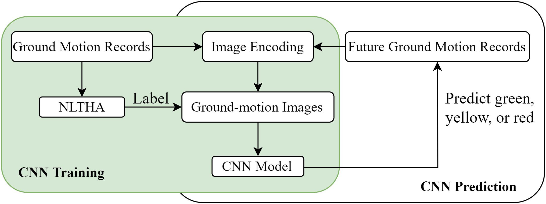
Figure 1. Methodology of the convolutional neural networks- (CNN) based seismic damage evaluation.

Different CNN architectures such as the AlexNet (Krizhevsky et al., 2012), VGG-Net (Simonyan and Zisserman, 2015), InceptionNet (Szegedy et al., 2015), ResNet (He et al., 2016), and DenseNet (Huang et al., 2017) were developed and utilized to identify thousands of subjects. These architectures were widely studied in Mangalathu and Jeon (2020) to evaluate the seismic damage via transfer learning (Pan and Yang, 2010). The main advantage of using these pre-trained CNN architecture lies in that it can train very deep neural networks with fewer data and less training time. However, since these pre-trained CNN architectures were mainly designed to identify hundreds, or even thousands of classes, they are generally very deep and have millions of learnable parameters to store after well-trained, which will cause a huge storage problem if they are utilized in regional seismic damage evaluation where thousands of CNN models need to be trained and stored. Besides, there are only three classes of green, yellow, and red tags in seismic damage evaluation. Therefore, we will propose a new CNN architecture in this paper (section “Convolutional Neural Networks Training and Results”), which has less than 20% (0.1–0.2 million parameters depending on the size of input images) of the learnable parameters used in the existing CNN architectures as discussed above.

Figure 2 shows the CNN architecture used in this study. A normal image consists of three channels – R (red), B (blue), and G (green), which store the brightness and color information of any subject in the image as pixel values. Similarly, a ground-motion image is also comprised of three channels – A (acceleration), V (velocity), and D (displacement). The AVD channels store the intensity and temporal (frequency) information of the ground motion as pixel values. These pixel values are inputted into the CNN model that is comprised of feature extraction layers and fully connected layers. The feature extraction layers are stacked with convolutional layers and pooling layers alternatively. Through the convolutional layers, new channels are generated via a small sliding window (e.g., 2 × 2, 3 × 3, or 5 × 5 depending on the image size) with learnable weights scanning over the image local pixels horizontally and vertically in a customized stride. ReLu activation function is usually adopted in the convolutional layer due to its computational efficiency (Li and Yuan, 2017). Through the pooling layers, a similar scanning technique to the convolutional layer is adopted to take the maximal or mean value of a local area on different channels for the purpose of down sampling. In this paper, the max pooling is adopted because it outperformed the mean pooling as demonstrated by Cha et al. (2017). Note that there are no weights to learn in the pooling layer. Examples of convolution and max pooling are given in Figure 2 to represent the detailed computation process. The horizontal and vertical output sizes of convolutional layers and pooling layers are determined by the corresponding input size in each orientation, the stride size, and the sliding window size as shown in the given examples. With carefully tuned weights of convolutional layers, the feature extraction layers can automatically extract the features of the input image and generate high level features for the fully connected layers. The fully connected layers of the CNN architecture take in the extracted features to identify the class of the input image.

FIGURE 2

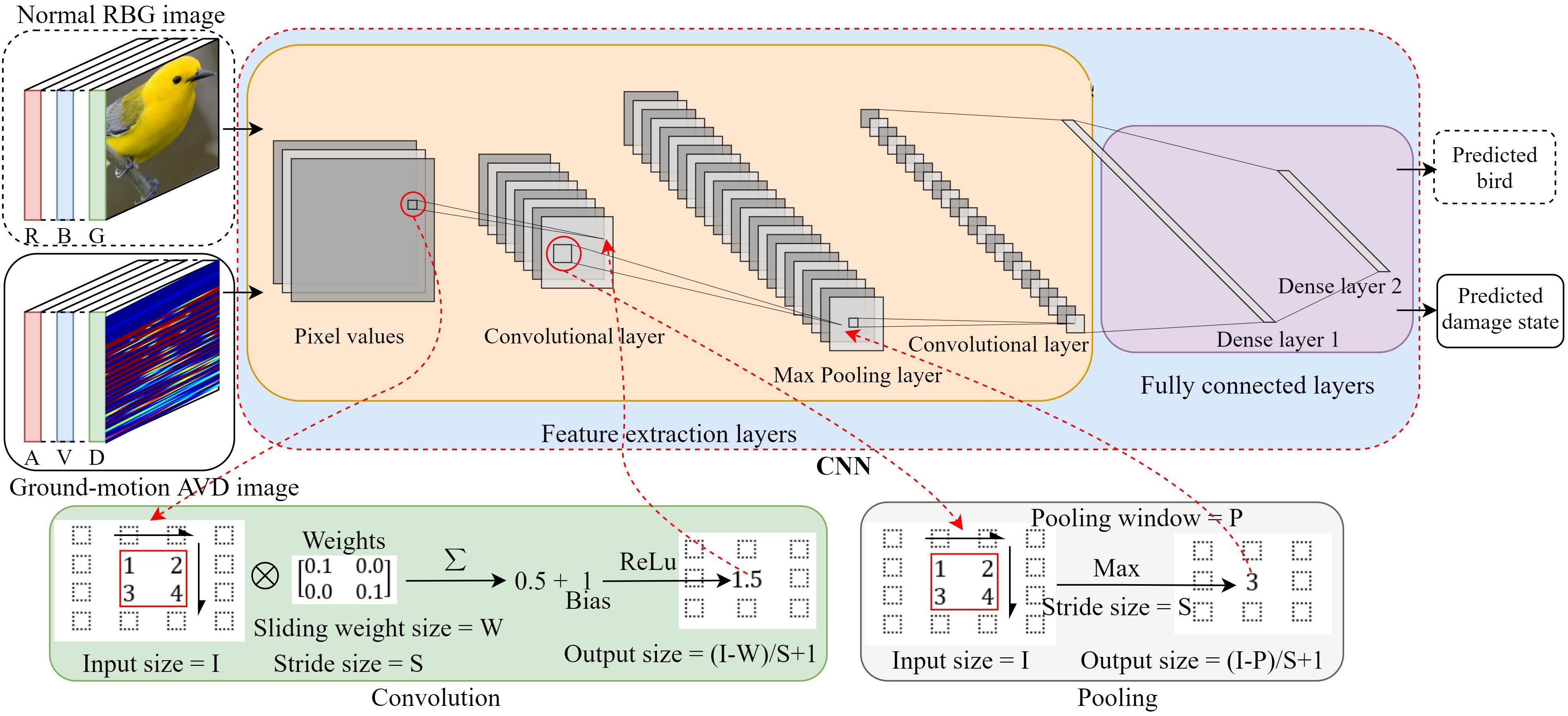
Figure 2. A CNN architecture to predict image classes. Features are automatically extracted in convolutional layers and max pooling layers. The extracted features are fed to the fully connected layers for prediction.

Image Encoding of Ground Motion Records

As seen in Figure 2, a ground-motion AVD image is comprised of A (acceleration), V (velocity), and D (displacement) channels. The ground motion information is represented as pixel values in the three channels. When Mangalathu and Jeon (2020) transformed the ground motion records into images via the WT technique, they considered ground accelerograms only. Therefore, their WT images were expressed in one channel with the recorded acceleration information of an earthquake event. However, the previous structural dynamics and earthquake engineering studies by Riddell (2007) and Chopra (2012) showed that the seismic responses of stiff and flexible structures with short, intermediate, and long natural periods are sensitive to the acceleration-, velocity-, and displacement-related characteristics of ground motions, respectively. To generate ground motion images that represent a wide frequency range of structures, the ground motion records are encoded into AVD images in three channels, where A, V, and D channels are transformed from the acceleration, velocity, and displacement records of an earthquake event. The new technique, TS, along with two state-of-the-art encoding techniques, RP and WT, are adopted to encode the AVD ground-motion images in this section.

Recurrence Plot

The RP technique can be used to visualize the periodic nature of a trajectory in a phase space and present certain aspects of the phase space trajectory in a 2D representation (Eckmann et al., 1987). The RP technique was proposed to encode time series as images for CNN classification by Debayle et al. (2018) and was found to outperform the traditional methods of time-series classification such as support vector machine (SVM) and the GAF–MTF encoding technique. The RP reveals times when the phase space trajectory of a dynamic system fluctuates around a constant phase. For a time series X = {x₁,x₂,x₃,…,x_n} with a certain time step, the phase space trajectory with a time delay embedding τ (multiplier of the time step) and dimension m is S = {s₁,s₂,s₃,…,s_{n−(m−1)τ}} in which vector s_i = (x_i,x_{i + τ},…,x_{i + (m−1)τ}). The RP can be mathematically presented in Eq 1,

$$R_{ij}=\mathrm{\theta }\left({\mathrm{\epsilon }}_i-||s_i-s_j||\right),i,j=1,\mathrm{\hspace{0.33em}2},\mathrm{\hspace{0.33em}3},\mathrm{\dots },n-(m-1)\mathrm{\tau }(1)$$

where ε_i is a threshold value, θ(⋅) is the Heaviside function, and ||⋅|| represents the norm of an argument in the bracket. With the Heaviside function, the 2D squared matrix R only consists of ones and zeros. Valuable information might be lost by the binarization of the R-matrix as pointed out by Debayle et al. (2018). To avoid the information loss, they skipped the Heaviside function and directly used the norm value ||s_i−s_j|| to form the 2D texture image. In this paper, we follow the same approach to directly generate the RP images of ground motion records. Note that the squared RP image size with a time delay embedding τ and dimension m of the state s_i is n−(m−1)τ, where n is the total number of data points in a time series.

Wavelet Transform

The Wavelet Transform (WT) can compute the temporal frequency feature of a time series at different locations in the duration by decomposing the time series into many wavelets that are localized in time and represent a narrow frequency range. There are two forms of WT: discrete wavelet transform (DWT) and continuous wavelet transform (CWT). Since CWT is advantageous over DWT in accurately estimating the instantaneous frequencies of signals with high resolution (Li et al., 2009), Mangalathu and Jeon (2020) used CWT to encode earthquake accelerograms as one-channel images for CNN classification. On the other hand, CWT was utilized to identify the pulse-like ground motions (Baker, 2007; Yaghmaei-Sabegh, 2010), where the ground-motion velocity records were encoded into images to classify near-fault ground motions. A brief overview of CWT on theoretical and algorithmic features (e.g., Heil and Walnut, 1989; Daubechies, 1990; Daubechies et al., 1992) is provided here. The CWT of a general time signal f(t) with a mother wavelet $\overline{\mathrm{\psi }}(\cdot )$ is defined in Eq 2,

$$W(a,b)=\frac{1}{\sqrt{a}}\underset{-\mathrm{\infty }}{\overset{+\mathrm{\infty }}{\int }}\overline{\mathrm{\psi }}\left(\frac{t-b}{a}\right)f\left(t\right)dt(2)$$

Where W(a,b) is the wavelet coefficient associated with a scale factor a and a time position factor b, and $\overline{\mathrm{\psi }}(\cdot )$ is the complex conjugate of the mother wavelet. A commonly used mother wavelet Morse wavelet (Olhede and Walden, 2002) used by Mangalathu and Jeon (2020) is also adopted in this paper. The coefficients W(a,b) are used to form a W matrix and generate the WT images of ground motion records. Since CWT computes the wavelet coefficients associated with every integer value of the scale and position parameters of a signal series X = {x₁,x₂,x₃,…,x_n} with length n, the WT image size is determined by the scale range (frequency range) and length of the time series.

Time-Series Segmentation

The RP and WT imaging techniques need to process the raw ground motion records and represent the recurrence values and wavelet values in texture images, respectively. As stated by Debayle et al. (2018), valuable information might be lost in the process of ground motion records. On the other hand, the size of WT time-series images is partially determined by the length of the time series. For a ground motion record whose strong motion over the 5–95% Arias Intensity duration could last for more than 200 s (s for second) with a sampling rate of over 50 Hz (Raghunandan and Liel, 2013), the length of the ground motion record can be more than ten of thousands data, which can make CNN training time-consuming because of the need for large-scale WT images. The accelerogram duration used in Mangalathu and Jeon (2020) was 30 s. Since the ground motion duration plays an import role in the collapse capacity of a structure (Raghunandan and Liel, 2013), it is not desirable to artificially reduce the ground motion duration to compensate for large scale data processing. Therefore, we propose the TS technique to encode ground motion records as texture images that can maintain their long duration while reducing their image size. Time-series segmentation has been widely used in time series analysis and mining (e.g., Chung et al., 2004; Lemire, 2007; Liu et al., 2008; Isensee et al., 2018). In this paper, we evenly divide the ground motion record into M pieces, each having a length N. M and N can be flexible when the 2D images are encoded and our examination shows that the overall classification accuracy is close when different Ms and Ns are used in the case study of section “Case Study of a Benchmark Building”. However, since square images (M = N) are usually adopted in existing deep learning CNN architectures like VGG-Net and ResNet because square images are easier to cope with the convolutional kernel and stride size, we encode the square 2D ground-motion images in this way as well. Thus, the raw acceleration, velocity, and displacement values can be stored in the matrix form and encoded as texture images for CNN training and validation. Note that it does not matter which orientation to stack these pieces into the matrix because the CNN model will scan the images both horizontally and vertically. The segmentation of the ground motions can significantly downsize the texture images while maintaining a long duration of the ground motion. For example, a ground motion record with 100 s duration and a sampling rate of 100 Hz has 10,000 data points. The texture image size can be only 100 × 100 if the original record is divided into 100 pieces. The formula of TS image is defined in Eq 3.

$$X=\{x_1,x_2,\mathrm{\dots },x_{M\times N}\}\stackrel{encoding}{\to }\left\{\begin{array}{c}{x}_1\\ x_{N+1}\\ ⋮\\ x_{(M-1)*N+1}\end{array}\begin{array}{c}{x}_2\\ x_{N+2}\\ ⋮\\ \cdots \end{array}\begin{array}{c}\cdots \\ \cdots \\ \ddots \\ \cdots \end{array}\begin{array}{c}{x}_N\\ x_{2N}\\ ⋮\\ x_{M\times N}\end{array}\right\}(3)$$

Acceleration, Velocity, and Displacement Images by RP, WT, and TS

The datasets from the UCR time series archival (Chen et al., 2015) used by Debayle et al. (2018) had a longest length of 637 points in Lightning2 time series. They adopted the time delay embedding τ = 4 and dimension m = 3 to encode 28 × 28, 56 × 56, and 64 × 64 RP images (very small). The ground motion acceleration records which were encoded with the WT by Mangalathu and Jeon (2020) were only 30 s long, of which the scale number and transition number were not given. As a matter of fact, the ground-motion image sizes can always be customized and uniformed according to the sampling parameters of the regional seismograph station in real engineering applications. In this paper, the proposed AVD images of ground motion records are encoded with RP, WT, and TS techniques in size of 500 × 500, 1,000 × 100, and 100 × 100, respectively. The acceleration, velocity, and displacement records of a ground motion with 100 s in duration and a sampling step of 0.01 s are transformed to the three-channel AVD images as shown in Table 1. Note that the length of the ground motion records reaches 10,000. When the RP technique is adopted, the time delay embedding τ = 95 and dimension m = 101 to significantly downsize the RP images for CNN training. When the WT technique is adopted, the ground motion records are resampled with a frequency of 10 Hz (0.1 s) to reduce the length to 1,000 and 100 scales from 0.05 to 50 with a 0.5 increment are used to generate the WT images. Since they have different durations and lengths, the ground motion records can be cut, resampled, or padded to make their length suitable for the pre-selected image size. Since the ground motion duration plays an important role in structural collapse (Raghunandan and Liel, 2013), we choose to resample the record with a different sampling frequency. In Table 1, the memory size of one image is also given with the unit of MegaByte (MB). It is evident that the TS AVD image takes the least memory space. To make a fair comparison between these techniques, we will also encode AVD images with 100 × 100 size via RP and WT in the case study of section “Case Study of a Benchmark Building” to investigate their performance for CNN seismic damage evaluation.

TABLE 1

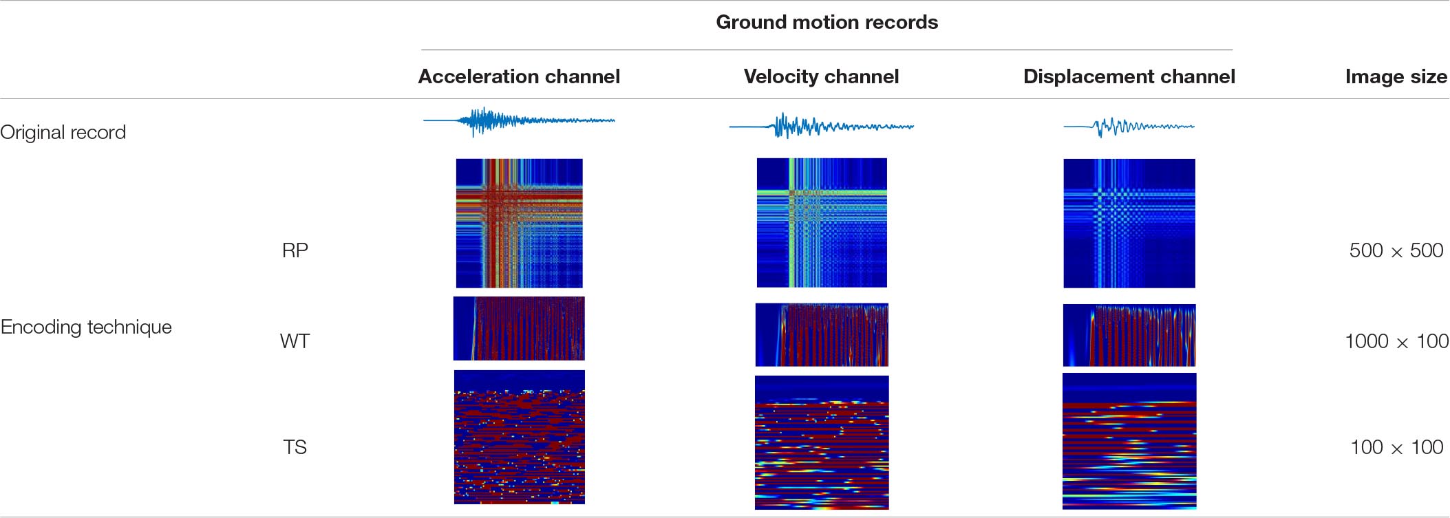
Table 1. Acceleration, velocity, and displacement (AVD) images of ground motion records by different image encoding techniques.

Case Study of a Benchmark Building

The Benchmark Building and Ground Motion Records

The CNN ground motion classifier with different image encoding techniques are investigated and compared using a reinforced concrete moment-frame (RCMF) benchmark building designed by Haselton et al. (2008) in compliance with the 2003 International Building Code (IBC). This code-conforming building is located in a high seismic zone in California. The rectangular building with 4 × 6 bays resists lateral loads through four moment-resisting frames around its perimeter. The elevation view of the perimeter frame is shown in Figure 3. Given that the lateral forces on the building are mainly resisted by the perimeter frames, the entire building is simplified into a 2D-frame structure. The perimeter frame in Figure 3 is simulated in the software OpenSEES (McKenna, 2011), where the columns and beams as described in Table 2 are represented by distributed-plasticity fiber elements. Nonlinear hysteretic characteristics of the element cross sections are captured by the uniaxial materials in OpenSEES, i.e., Concrete02 material model for unconfined and confined concrete (nominal compressive strength 35 MPa), and Steel02 material model for Grade 60 steel reinforcement (nominal yield strength 460 MPa), respectively. The columns of the frame structure are fixed on the ground. The modal analysis shows that the simplified structure has a fundamental period of 0.724 s. Details of the structural and non-structural design, and the more sophisticated computational model are referred to the original report (Haselton et al., 2008).

FIGURE 3

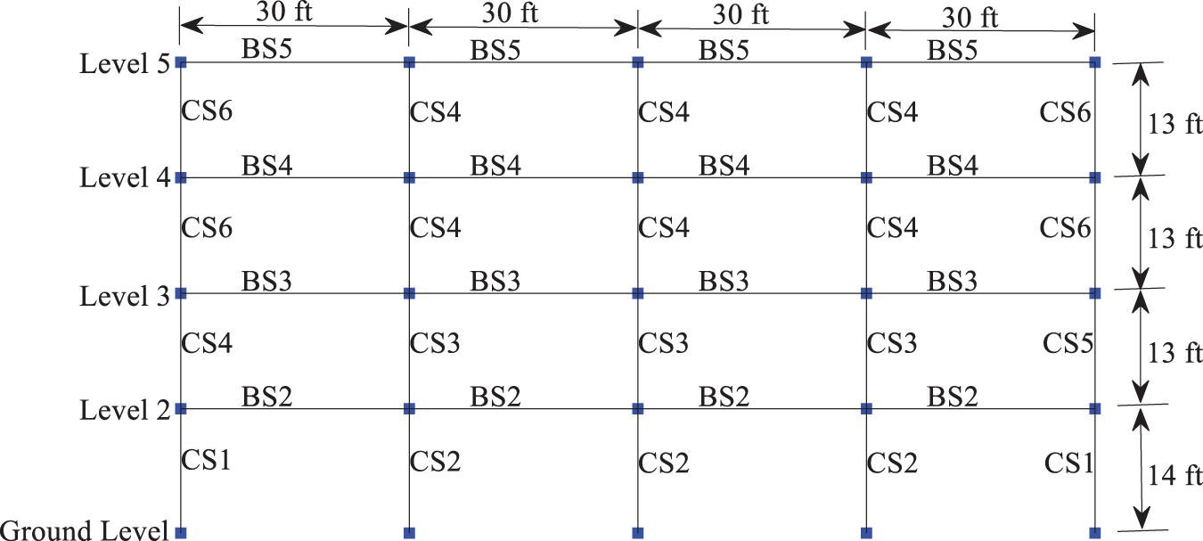
Figure 3. The elevation view of the benchmark structure (1 ft = 3.3 m).

TABLE 2

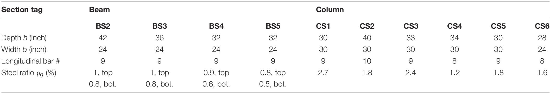
Table 2. Column and beam dimension and reinforcement properties (1 inch = 25.4 mm, bot. = bottom).

The structural model in Figure 3 is subjected to a suit of ground motions in NLTHA to generate their ATC-40 tags associated with various degrees of structural damage (Applied Technology Council, 1996). To obtain enough training samples for each damage tag, i.e., green, yellow, and red, a total of 1,993 ground acceleration records with a peak ground acceleration (PGA) of higher than 0.15 g (g = 9.81 m/s²) are selected from the Pacific Earthquake Engineering Research Center (PEER) database¹. When code-conformed with the most stringent seismic design requirements, the frame structure experiences severe damage only under a few of the 1,993 historical ground motion records. Therefore, the ground motion records are scaled by 2–10 times in amplitude with an increment of 1, as commonly adopted in the seismology community (Luco and Bazzurro, 2007). In addition, 2,500 synthetic accelerograms are generated based on a spectrum- and energy-compatible algorithm (Li et al., 2017), totaling the 22,430 ground acceleration records collected. These ground acceleration records are inputted into the frame model and labeled with the green, yellow, and red tags based on their resulting maximal interstory drift ratio (MIDR). According to the analysis results of Haselton et al. (2008), the benchmark frame would experience a MIDR of 0.005–0.02 under design ground motions with 10% probability of exceedance in 50 years, which meets the design code requirements. The MIDR at collapse would be in the order of 0.07–0.12. The solution for MIDR beyond 0.12 is deemed unrealistic due to the dynamic instability of the collapsed structure and the corresponding ground motion records are thus excluded from further analysis. This decision is also supported by the conclusion drawn by Luco and Bazzurro (2007) as excessive scaling of the ground motion records would introduce bias to the seismic NLTHA results. Next, the ground motion records are labeled with a green, yellow, and red tag when they result in MIDR < 0.02, 0.02 ≤ MIDR < 0.05, and 0.05 ≤ MIDR, respectively. The selection of 0.05 as a lower bound MIDR for the red tag corresponds to an approximate mean minus three times standard deviation of 353 MIDR data points in the range of 0.07–0.12. Finally, a balanced dataset of 3,201 ground motion records, each class containing 1,067 samples, is obtained to ensure that the adequate and equal training samples are fed to the CNN model.

Convolutional Neural Networks Training and Results

The RP, WT, and TS techniques are applied to the 3,201 ground motion records to generate 3,201 AVD ground-motion images and are fed to the CNN model for training and validation. The 3,201 images are split into two sets for training and validation. The training set consists of 2,250 images, each class including 750 images. The validation set contains 951 images, each class having 317 images. The validation set is meant to test the performance of the CNN model on unseen data to avoid overtraining. All trainings are carried out on the MATLAB platform (MATLAB, 2018) using a workstation with Intel (R) Xeon (R) Gold 6148 CPU @2.4 GHz, 2 GPU NAVID Quadro P5000, and 192G memory. As illustrated in Figure 2, the CNN architecture is comprised of three convolutional layers and two max pooling layers that are alternated to extract features, and two fully connected layers to predict the class of ground-motion images. The three convolutional layers have 128, 64, and 32 channels, respectively. For each convolutional layer, the convolution windows have a size of 3 × 3 and a stride of 2. The two intermediate pooling layers contain a pooling window of 2 × 2 and a stride of 2. The loss function of categorical crossentropy and the optimizer rmsprop are adopted. Since it remains an open problem to find the optimal CNN parameters (Debayle et al., 2018), the CNN parameters in this study are determined mainly based on their performance on the validation dataset and the guidance from the computing platform. After the CNN architecture is built, the RP-based AVD images with a size of 100 × 100 and 500 × 500, the WT-based AVD images with a size of 100 × 100 and 1,000 × 100, and the TS-based AVD images with a size of 100 × 100 are, respectively, fed to the CNN model for proper training. An example of the TS-based CNN training history is shown in Figure 4. The total training goes through 8 training epochs of 35 iterations each using a single GPU and a learning rate of 0.0001. The total training time is 33 s. The performance of the CNN model rapidly converges in the first few epochs, and training is stopped when the validation loss starts to increase to avoid the overtraining of the CNN model. If overtrained, the CNN model will lose performance on the unseen data of future ground motions.

FIGURE 4

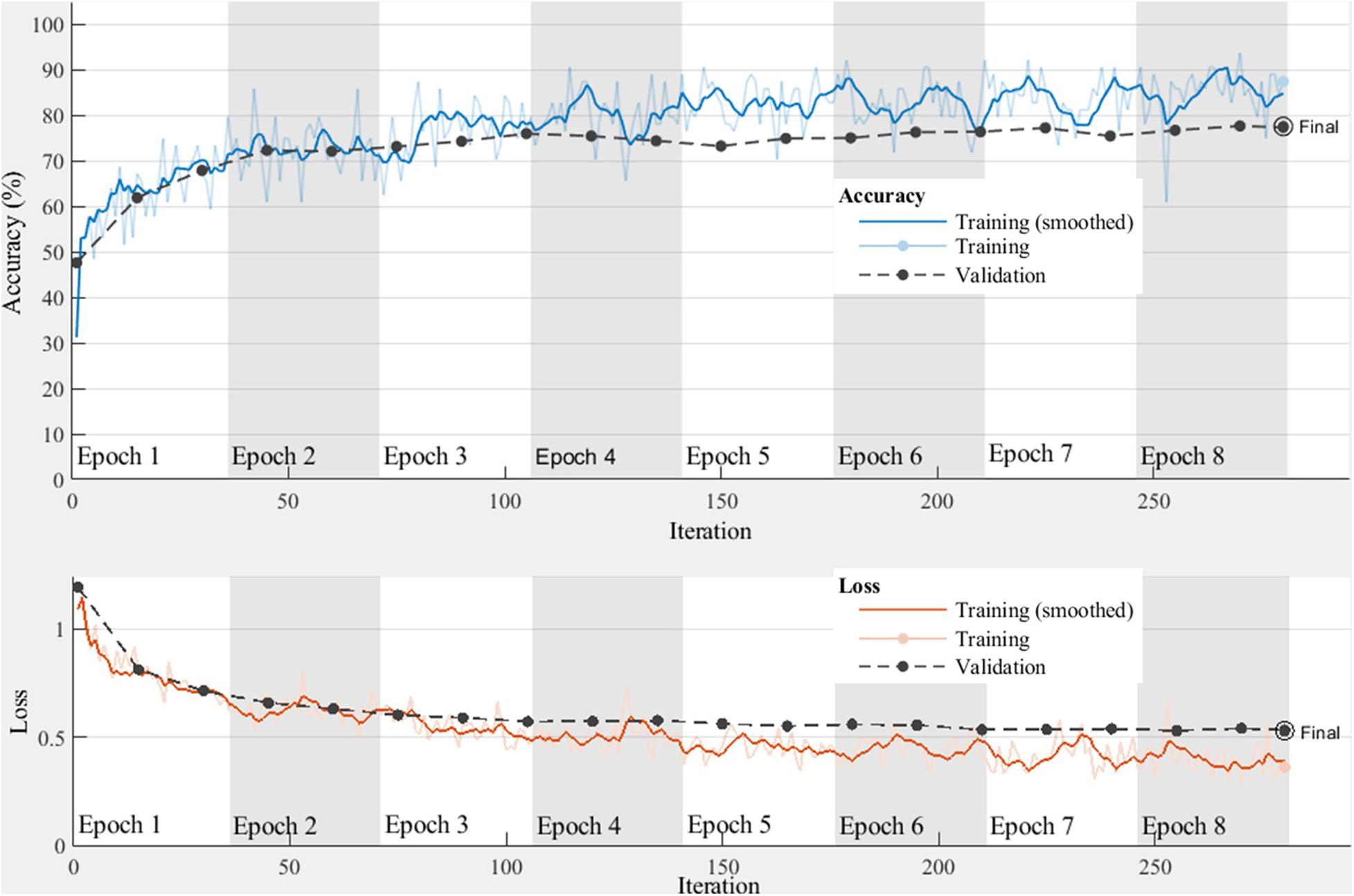
Figure 4. Accuracy and loss histories of the TS-based CNN model. For both training and validation datasets, the loss histories are decreasing, indicating that the CNN model is properly trained without overfitting. One epoch means all training samples are fed to the CNN model once before the next training iteration starts.

Figure 5 shows the classification results of the training and validation datasets from the trained TS-based CNN model. Consider the validation dataset of 951 AVD images as shown in Figure 5B. The confusion matrix includes a total of 951 prediction classes, each row for one prediction class and each column for one true class. In the second row of the validation matrix, the CNN model predicts 299 images as yellow tags (ground motion images), including 100 false positive cases (42 for green tags and 58 for red tags). The true positive ratio in the second row is 66.6%, known as precision ratio p_–ratio. In the second column of the validation matrix, among 317 true yellow tags, 199 samples are correctly classified while 44 are misclassified as green cases, and 74 as red cases. The correct classification ratio in the second column is 62.8%, known as recall ratio r_–ratio. Given in the right bottom corner of the matrix, the overall classification accuracy of the TS-based CNN model is 76.8%, which represents a ratio of the correctly classified cases and the 951 cases in the whole validation dataset. A compound index F_–measure of the p_–ratio and r_–ratio, and the overall classification accuracy are thus used to evaluate the performance of the CNN model. The F_–measure is defined as Eq 4,

FIGURE 5

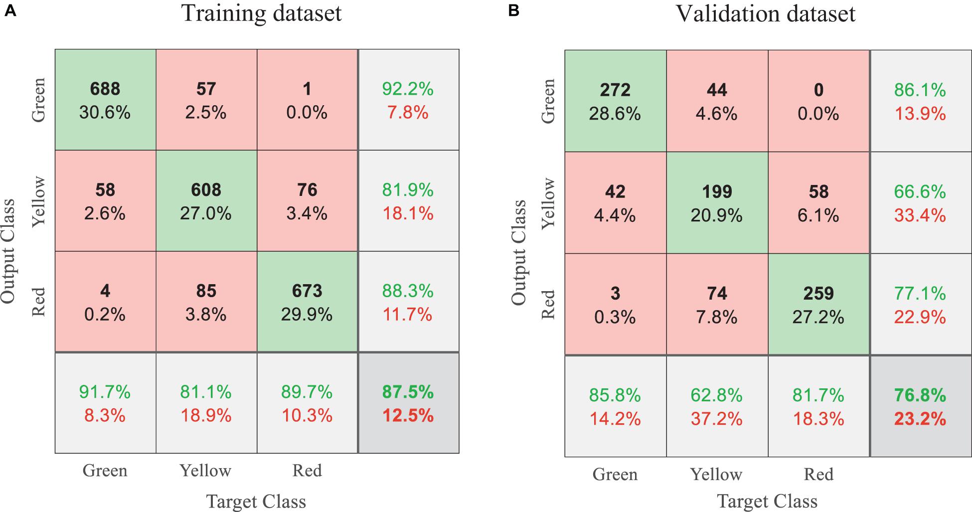
Figure 5. Classification results summarized in confusion matrices for: (A) the training dataset; (B) the validation dataset.

$$F_{-measure}=\left(1+{\mathrm{\beta }}^2\right)\frac{p_{-ratio}\cdot r_{-ratio}}{{\mathrm{\beta }}^2{p}_{-ratio}+r_{-ratio}}(4)$$

Where β indicates that r_–ratio is β times as important as p_–ratio. We set β = 1 because in the task of seismic damage evaluation, most true positive cases in each damage class should be identified without raising too many false alarms.

In Figure 5, the classification results indicate that the CNN model performs better on the training dataset than the validation dataset, which matches the observation in Figure 4. This is because the samples in the training dataset have already been fed to the CNN model and have been specifically learnt by the model. The validation data is more representative of future data, as the model has not seen them. Therefore, the F_–measure and accuracy of the validation dataset are used to evaluate and compare the performance of various CNN models based on different image encoding techniques in section “Results and Discussion.” A F_–measure and accuracy closer to 1 means better classification results.

Results and Discussion

The five CNN models taking the RP-based AVD images with a size of 100 × 100 and 500 × 500, the WT-based AVD images with a size of 100 × 100 and 1,000 × 100, and the TS-based AVD images with a size of 100 × 100 are compared among themselves and with two state-of-the-art machine-learning models: logistic regression (LR) and decision tree (DT). This is because the LR algorithm is highly accurate and efficient while the DT algorithm is less efficient but easier to interpret (Xu et al., 2020b). In their study, Xu et al. (2020b) also recommended several IMs from a pool of 48 IMs to be used in the machine-learning models for effective damage evaluation, including the spectral acceleration at the fundamental period of a target structure, effective peak acceleration, Housner intensity, effective peak velocity, and peak ground velocity, that are used in this study to train the LR and DT machine learning models. Figure 6 presents the F_–measure values and the overall accuracy of the validation dataset corresponding to the classification results of the five CNN models and the two machine learning models. The CNN model based on the WT 1,000 × 100 AVD images and the machine-learning LR model predict the best classification results or generate the two highest values in Figure 6. The CNN models based on the RP 500 × 500 and TS 100 × 100 AVD images and the machine-learning DT model generate the second-best results. The CNN models based on WT 100 × 100 and RP 100 × 100 AVD images perform worst in classification. Further examination on the two most accurate models indicates that the features of ground motion records automatically extracted by the CNN architecture with the WT 1,000 × 100 AVD images (in contrast to the machine-learning LR model) can lead to a slightly more accurate damage classification on the post-earthquake structural damage states. Therefore, the proposed CNN architecture with far less learnable parameters can achieve the same or better classification results. Additionally, the smaller size of learnable parameters is promising for large-scale regional seismic evaluation that requires models to be saved and run in real time.

FIGURE 6

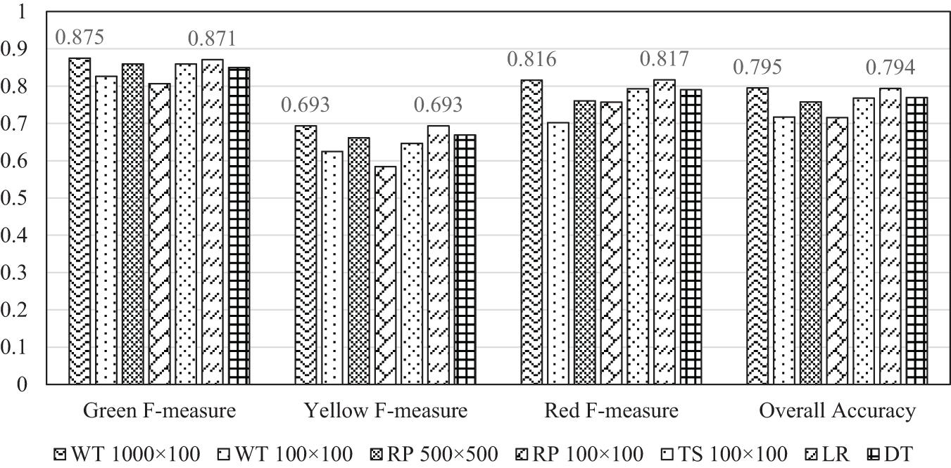
Figure 6. Classification performance comparison of different models according to the F-measure of each damage class and overall accuracy. The overall accuracy (79.5%) of the CNN model trained with WT 1,000 × 100 AVD images is slightly higher than that (79.4%) of the IM-based machine learning LR model.

Table 3 shows the time spent in CNN model training with different AVD images. The entire training process is completed on the MATLAB platform using a workstation with the same CNN parameter setting as previously mentioned in section “Convolutional Neural Networks Training and Results”. It is evident from Table 3 that the larger the AVD image size, the more costly the computational time to encode the image and train its corresponding CNN model. While the validation accuracy (76.8%) of the TS 100 × 100 encoding technique is lower than that (79.5%) of the WT 1,000 × 100 technique, the TS 100 × 100 technique is most computationally efficient in encoding, training, and testing. The WT 1,000 × 100 and the TS 100 × 100 encoding methods are thus recommended for future study. Note that the prediction of each AVD image only consumes 4.14 ms for the WT encoding technique and 0.36 ms for the proposed TS technique. Therefore, once the CNN models of target structures are well trained, they can be used to run near real-time damage evaluation for future earthquake events.

TABLE 3

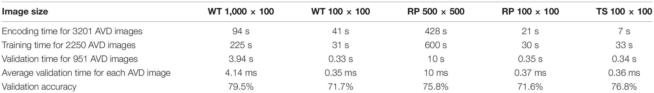
Table 3. Computational efficiency comparison of convolutional neural networks (CNN) models trained with different AVD images.

Conclusion

Automatic feature extraction from a large set of complex ground motion data and proper encoded image size (width × height × channel) are important in CNN-based seismic damage evaluation. A new TS image encoding technique has been developed to transform acceleration, velocity, and displacement ground motion records into an AVD image of the ground motion event for seismic classification evaluation. The new TS has been compared with two state-of-the-art image encoding techniques, namely RP and WT. While the classification accuracy of the CNN trained with 2,250 ground motion images slightly decreases from 79.5% when using the WT 1,000 × 100 image encoding technique to 76.8% when using the TS 100 × 100 encoding technique, the validation time for 951 AVD images is reduced by 11.6 times from 3.94 to 0.34 s. Both classification accuracies are comparable to 79.4% from the IM-based LR model.

For small-scale training with limited structures or ground motion records, we recommend WT 1,000 × 100 for better accuracy. For large-scale training, we recommend TS 100 × 100 for higher efficiency while maintaining the same order of accuracy. With an increasing AVD image size, it costs more time to encode the ground motion and train the corresponding CNN model with more learnable parameters. Overall, the CNN-based seismic damage prediction of each AVD image only costs less than 5 ms. Once the CNN models of target structures are well trained, they can be saved to run near-real-time damage evaluation for future earthquake events.

The objective to explore suitable image encoding techniques and corresponding image sizes for CNN-based seismic damage evaluation based on a specific code-conforming benchmark building is achieved in this study. However, more research must be conducted to understand the effect of different types of structures (e.g., bridges) on CNN training and validation, and in particular the influences of material, geometry, and structural capacity uncertainties on the CNN classification accuracy. Even so, the three-channel WT-based AVD images with a size of 1,000 (width) × 100 (height) and TS 100 × 100 show great potential for CNN-based seismic damage evaluation.

Data Availability Statement

The raw data supporting the conclusions of this article may be made available upon request from the correspondence author.

Author Contributions

XY contributed to methodology of the study. XY and DT contributed to the CNN model training. XY and PJ performed the numerical simulation of the building. XY wrote the first draft of the manuscript. LL, GC, DW, DT, and XY contributed to manuscript revision and read. All authors approved the submitted version.

Funding

Financial support to complete this study was provided in part by the US Department of Transportation, Office of the Assistant Secretary for Research and Technology under the auspices of Mid-America Transportation Center at the University of Nebraska-Lincoln (Grant No. 00059709). Partial support for this research was received from the Missouri University of Science and Technology Intelligent Systems Center, the Mary K. Finley Missouri Endowment, the National Science Foundation, the Lifelong Learning Machines program from DARPA/Microsystems Technology Office, the Army Research Laboratory (ARL), and the Leonard Wood Institute; and it was accomplished under Cooperative Agreement Numbers W911NF-18-2-0260 and W911NF-14-2-0034. The views and conclusions contained in this document are those of the authors and should not be interpreted as representing the official policies, either expressed or implied, of the Leonard Wood Institute, the National Science Foundation, the Army Research Laboratory, or the U.S. Government.

Disclaimer

The U.S. Government is authorized to reproduce and distribute reprints for Government purposes notwithstanding any copyright notation herein.

Conflict of Interest

The authors declare that the research was conducted in the absence of any commercial or financial relationships that could be construed as a potential conflict of interest.

Acknowledgments

The kind help from Drs. Jun Han and Haibin Zhang during the completion of this paper is highly appreciated. The reviews and comments by reviewers are highly appreciated.

Footnotes

1. ^ https://ngawest2.berkeley.edu/

References

Applied Technology Council. (1996). ATC 40 Seismic Evaluation and Retrofit of Concrete Buildings. Redwood City CA: Seismic Safety Commisionsion.

Google Scholar

Baker, J. W. (2007). Quantitative classification of near-fault ground motions using wavelet analysis. Bulletin of the Seismological Society of America. 97, 1486–1501. doi: 10.1785/0120060255

CrossRef Full Text | Google Scholar

Baker, J. W., and Cornell, C. A. (2005). A vector-valued ground motion intensity measure consisting of spectral acceleration and epsilon. Earthquake Engineering and Structural Dynamics. 34, 1193–1217. doi: 10.1002/eqe.474

CrossRef Full Text | Google Scholar

Cha, Y. J., Choi, W., and Büyüköztürk, O. (2017). Deep Learning-Based Crack Damage Detection Using Convolutional Neural Networks. Computer-Aided Civil and Infrastructure Engineering. 32, 361–378. doi: 10.1111/mice.12263

CrossRef Full Text | Google Scholar

Chen, Y., Keogh, E., Hu, B., Begum, N., Bagnall, A., Mueen, A., et al. (2015). The UCR Time Series Classification Archive. Available online at: www.cs.ucr.edu/~eamonn/time_series_data/ (accessed January 5, 2021).

Google Scholar

Chopra, A. K. (2012). Dynamics of structures. Upper Saddle River, NJ: Pearson Education.

Google Scholar

Chung, F. L., Fu, T. C., Ng, V., and Luk, R. W. (2004). An evolutionary approach to pattern-based time series segmentation. IEEE Transactions on Evolutionary Computation. 8, 471–489. doi: 10.1109/TEVC.2004.832863

CrossRef Full Text | Google Scholar

Cimellaro, G. P., Reinhorn, A. M., and Bruneau, M. (2010). Seismic resilience of a hospital system. Structure and Infrastructure Engineering. 6, 127–144. doi: 10.1080/15732470802663847

CrossRef Full Text | Google Scholar

Daubechies, I. (1990). The Wavelet Transform, Time-Frequency Localization and Signal Analysis. IEEE Transactions on Information Theory. 36, 961–1005. doi: 10.1109/18.57199

CrossRef Full Text | Google Scholar

Daubechies, I., Barlaud, M., and Mathieu, P. (1992). Image Coding Using Wavelet Transform. IEEE Transactions on Image Processing. 1, 205–220. doi: 10.1109/83.136597

CrossRef Full Text | Google Scholar

Debayle, J., Hatami, N., and Gavet, Y. (2018). “Classification of time-series images using deep convolutional neural networks,” in Proceedings of the 10th International Conference on Machine Vision (ICMV 2017) (Vienne: SPIE), doi: 10.1117/12.2309486

CrossRef Full Text | Google Scholar

Du, A., Padgett, J. E., and Shafieezadeh, A. (2020). Influence of intensity measure selection on simulation-based regional seismic risk assessment. Earthquake Spectra. 36, 647. doi: 10.1177/8755293019891717

CrossRef Full Text | Google Scholar

Eckmann, J. P., Oliffson Kamphorst, O., and Ruelle, D. (1987). Recurrence plots of dynamical systems. EPL 4, 973–977. doi: 10.1209/0295-5075/4/9/004

CrossRef Full Text | Google Scholar

Grigoriu, M. (2016). Do seismic intensity measures (IMs) measure up? Probabilistic Engineering Mechanics 46, 80–93. doi: 10.1016/j.probengmech.2016.09.002

CrossRef Full Text | Google Scholar

Haselton, C. B., Goulet, C. A., Mitrani-Reiser, J., Beck, J. L., Deierlein, G. G., Porter, K. A., et al. (2008). An assessment to benchmark the seismic performance of a code-conforming reinforced concrete moment-frame building, PEER report. Berkeley, CA: Pacific Earthquake Engineering Research Center.

Google Scholar

He, K., Zhang, X., Ren, S., and Sun, J. (2016). “Deep residual learning for image recognition,” in Proceedings of the IEEE Computer Society Conference on Computer Vision and Pattern Recognition (Las Vegas, NV: IEEE), doi: 10.1109/CVPR.2016.90

CrossRef Full Text | Google Scholar

Heil, C. E., and Walnut, D. F. (1989). Continuous and discrete wavelet transforms. SIAM Review. 31, 628–666. doi: 10.1137/1031129

CrossRef Full Text | Google Scholar

Huang, G., Liu, Z., Van Der Maaten, L., and Weinberger, K. Q. (2017). “Densely connected convolutional networks,” in Proceedings of the 30th IEEE Conference on Computer Vision and Pattern Recognition, CVPR 2017 (Honolulu, HI: IEEE), doi: 10.1109/CVPR.2017.243

CrossRef Full Text | Google Scholar

Hwang, H., Liu, J. B., and Chiu, Y. H. (2001). “Seismic Fragility Analysis of Highway Bridges,” in Proceedings of the 9th ASCE Specialty Conference on Probabilistic Mechanics and Structural Reliability (Reston, VA: ASCE).

Google Scholar

Isensee, F., Jaeger, P. F., Full, P. M., Wolf, I., Engelhardt, S., and Maier-Hein, K. H. (2018). “Automatic cardiac disease assessment on cine-MRI via time-series segmentation and domain specific features,” in Lecture Notes in Computer Science (including subseries Lecture Notes in Artificial Intelligence and Lecture Notes in Bioinformatics) (Cham: Springer), doi: 10.1007/978-3-319-75541-0_13.

CrossRef Full Text | Google Scholar

Jalayer, F., Elefante, L., De Risi, R., and Manfredi, G. (2014). “Cloud analysis revisited: Efficient fragility calculation and uncertainty propagation using simple linear regression,” in Proceedings of the 10th U.S. National Conference on Earthquake Engineering NCEE 2014: Frontiers of Earthquake Engineering (Anchorage, AK: NCEE), doi: 10.4231/D3SF2MC59

PubMed Abstract | CrossRef Full Text | Google Scholar

Jalayer, F., Ebrahimian, H., Miano, A., Manfredi, G., and Sezen, H. (2017). Analytical fragility assessment using unscaled ground motion records. Earthquake Engineering and Structural Dynamics. 46, 2639–2663. doi: 10.1002/eqe.2922

CrossRef Full Text | Google Scholar

Kostinakis, K., Athanatopoulou, A., and Morfidis, K. (2015). Correlation between ground motion intensity measures and seismic damage of 3D R/C buildings. Engineering Structures. 82, 151–167. doi: 10.1016/j.engstruct.2014.10.035

CrossRef Full Text | Google Scholar

Krizhevsky, A., Sutskever, I., and Hinton, G. E. (2012). ImageNet classification with deep convolutional neural networks. Advances in Neural Information Processing Systems 25, 1097–1105.

Google Scholar

Kussul, E. M., Baidyk, T. N., Wunsch, D. C., Makeyev, O., and Martín, A. (2006). Permutation coding technique for image recognition systems. IEEE Trans. Neural Networks 17, 1566–1579.

Google Scholar

Kwon, O. S., and Elnashai, A. (2006). The effect of material and ground motion uncertainty on the seismic vulnerability curves of RC structure. Engineering Structures 28, 289–303. doi: 10.1016/j.engstruct.2005.07.010

CrossRef Full Text | Google Scholar

LeCun, Y., Bottou, L., Bengio, Y., and Haffner, P. (1998). Gradient-based learning applied to document recognition. Proceedings of the IEEE 86, 2278–2324. doi: 10.1109/5.726791

CrossRef Full Text | Google Scholar

Lecun, Y., Bengio, Y., and Hinton, G. (2015). Deep learning. Nature. 521, 436–444. doi: 10.1038/nature14539

PubMed Abstract | CrossRef Full Text | Google Scholar

LeCun, Y., Kavukcuoglu, K., and Farabet, C. (2010). “Convolutional networks and applications in vision,” in Proceedings of the 2010 IEEE International Symposium on Circuits and Systems ISCAS: Nano-Bio Circuit Fabrics and Systems (Paris: IEEE), doi: 10.1109/ISCAS.2010.5537907

CrossRef Full Text | Google Scholar

Lemire, D. (2007). “A better alternative to piecewise linear time series segmentation,” in Proceedings of the 7th SIAM International Conference on Data Mining (Philadelphia, PA: SIAM), doi: 10.1137/1.9781611972771.59

CrossRef Full Text | Google Scholar

Li, H., Yi, T., Gu, M., and Huo, L. (2009). Evaluation of earthquake-induced structural damages by wavelet transform. Progress in Natural Science. 19, 461–470. doi: 10.1016/j.pnsc.2008.09.002

CrossRef Full Text | Google Scholar

Li, L., Fan, Y., Huang, X., and Tian, L. (2016). “Real-time UAV weed scout for selective weed control by adaptive robust control and machine learning algorithm,” in Proceedings of the 2016 American Society of Agricultural and Biological Engineers Annual International Meeting (St. Joseph, MI: ASABE), doi: 10.13031/aim.20162462667

CrossRef Full Text | Google Scholar

Li, Y., and Yuan, Y. (2017). Convergence analysis of two-layer neural networks with RELU activation. Advances in Neural Information Processing Systems 30, 597–607.

Google Scholar

Li, Z., Kotronis, P., and Wu, H. (2017). Simplified approaches for Arias Intensity correction of synthetic accelerograms. Bulletin of Earthquake Engineering. 15, 4067–4087. doi: 10.1007/s10518-017-0126-6

CrossRef Full Text | Google Scholar

Liu, X., Lin, Z., and Wang, H. (2008). Novel online methods for time series segmentation. IEEE Transactions on Knowledge and Data Engineering. 20, 1616–1626. doi: 10.1109/TKDE.2008.29

CrossRef Full Text | Google Scholar

Luco, N., and Bazzurro, P. (2007). Does amplitude scaling of ground motion records result in biased nonlinear structural drift responses? Earthquake Engineering and Structural Dynamics. 36, 1813–1835. doi: 10.1002/eqe.695

CrossRef Full Text | Google Scholar

Mangalathu, S., and Jeon, J.-S. (2020). Ground Motion-Dependent Rapid Damage Assessment of Structures Based on Wavelet Transform and Image Analysis Techniques. Journal of Structural Engineering. 146, 0402020230. doi: 10.1061/(asce)st.1943-541x.0002793

PubMed Abstract | CrossRef Full Text | Google Scholar

Mangalathu, S., Jeon, J. S., and DesRoches, R. (2018). Critical uncertainty parameters influencing seismic performance of bridges using Lasso regression. Earthquake Engineering and Structural Dynamics. 47, 784–801. doi: 10.1002/eqe.2991

CrossRef Full Text | Google Scholar

MATLAB. (2018). (R2018b). Natick, MA: The MathWorks Inc.

Google Scholar

McKenna, F. (2011) OpenSees: A framework for earthquake engineering simulation. Comput. Sci. Eng. 13, 58–66. doi: 10.1109/MCSE.2011.66

CrossRef Full Text | Google Scholar

Miano, A., Jalayer, F., Ebrahimian, H., and Prota, A. (2018). Cloud to IDA: Efficient fragility assessment with limited scaling. Earthquake Engineering and Structural Dynamics. 47, 1124–1147. doi: 10.1002/eqe.3009

CrossRef Full Text | Google Scholar

Morfidis, K., and Kostinakis, K. (2018). Approaches to the rapid seismic damage prediction of r/c buildings using artificial neural networks. Engineering Structures. 165, 120–141. doi: 10.1016/j.engstruct.2018.03.028

CrossRef Full Text | Google Scholar

Morfidis, K., and Kostinakis, K. (2019). Comparative evaluation of MFP and RBF neural networks ability for instant estimation of r/c buildings seismic damage level. Engineering Structures. 197, 109436. doi: 10.1016/j.engstruct.2019.109436

CrossRef Full Text | Google Scholar

Olhede, S. C., and Walden, A. T. (2002). Generalized Morse wavelets. IEEE Transactions on Signal Processing. 50, 2661–2670. doi: 10.1109/TSP.2002.804066

CrossRef Full Text | Google Scholar

Padgett, J. E., and DesRoches, R. (2007). Sensitivity of Seismic Response and Fragility to Parameter Uncertainty. Journal of Structural Engineering. 133, 1710–1718. doi: 10.1061/(asce)0733-94452007133:121710

CrossRef Full Text | Google Scholar

Padgett, J. E., Nielson, B. G., and DesRoches, R. (2008). Selection of optimal intensity measures in probabilistic seismic demand models of highway bridge portfolios. Earthquake Engineering and Structural Dynamics. 37, 711–725. doi: 10.1002/eqe.782

CrossRef Full Text | Google Scholar

Pan, S. J., and Yang, Q. (2010). A survey on transfer learning. IEEE Transactions on Knowledge and Data Engineering. 22, 1345–1359. doi: 10.1109/TKDE.2009.191

CrossRef Full Text | Google Scholar

Raghunandan, M., and Liel, A. B. (2013). Effect of ground motion duration on earthquake-induced structural collapse. Structural Safety. 41, 119–133. doi: 10.1016/j.strusafe.2012.12.002

CrossRef Full Text | Google Scholar

Riddell, R. (2007). On ground motion intensity indices. Earthquake Spectra. 23, 147. doi: 10.1193/1.2424748

CrossRef Full Text | Google Scholar

Simonyan, K., and Zisserman, A. (2015). “Very deep convolutional networks for large-scale image recognition,” in Proceedings of the 3rd International Conference on Learning Representations, ICLR 2015 Conference Track Proceedings (Vienna: ICLR).

Google Scholar

Szegedy, C., Liu, W., Jia, Y., Sermanet, P., Reed, S., Anguelov, D., et al. (2015). “Going deeper with convolutions,” in Proceedings of the IEEE Computer Society Conference on Computer Vision and Pattern Recognition (Boston, MA: IEEE), doi: 10.1109/CVPR.2015.7298594

CrossRef Full Text | Google Scholar

USGS. (2021). Real-time Seismogram Displays. USGS, Available online at: https://earthquake.usgs.gov/monitoring/seismograms (accessed January 3, 2021).

Google Scholar

Wald, D. J., Worden, B. C., Quitoriano, V., and Pankow, K. L. (2006). ShakeMap Manual: Technical Manual, Users Guide, and Software Guide. Reston, VA: USGS.

Google Scholar

Wang, Z., Pedroni, N., Zentner, I., and Zio, E. (2018). Seismic fragility analysis with artificial neural networks: Application to nuclear power plant equipment. Engineering Structures. 162, 213–225. doi: 10.1016/j.engstruct.2018.02.024

CrossRef Full Text | Google Scholar

Wang, Z., and Oates, T. (2015a). “Encoding time series as images for visual inspection and classification using tiled convolutional neural networks,” in Proceedings of the 29th AAAI Conference on Artificial Intelligence (Menlo Park, CA: AAAI).

Google Scholar

Wang, Z., and Oates, T. (2015b). “Imaging time-series to improve classification and imputation,” in Proceedings of the IJCAI International Joint Conference on Artificial Intelligence (Buenos Aires: IJCAI).

Google Scholar

Xie, Y., Ebad Sichani, M., Padgett, J. E., and DesRoches, R. (2020). The promise of implementing machine learning in earthquake engineering: A state-of-the-art review. Earthquake Spectra. 36, 1769–1801. doi: 10.1177/8755293020919419

CrossRef Full Text | Google Scholar

Xu, J. G., Wu, G., Feng, D. C., Cotsovos, D. M., and Lu, Y. (2020a). Seismic fragility analysis of shear-critical concrete columns considering corrosion induced deterioration effects. Soil Dynamics and Earthquake Engineering. 134, 106165. doi: 10.1016/j.soildyn.2020.106165

CrossRef Full Text | Google Scholar

Xu, Y., Lu, X., Tian, Y., and Huang, Y. (2020b). Real-Time Seismic Damage Prediction and Comparison of Various Ground Motion Intensity Meassures Based on Machine Learning. Journal of Earthquake Engineering doi: 10.1080/13632469.2020.1826371

CrossRef Full Text | Google Scholar

Yaghmaei-Sabegh, S. (2010). Detection of pulse-like ground motions based on continues wavelet transform. Journal of Seismology. 14, 715–726. doi: 10.1007/s10950-010-9193-8

CrossRef Full Text | Google Scholar