Performance-Based Coastal Engineering Framework

Introduction

Coastal communities face severe socio-economic challenges posed by the disastrous impacts of natural hazards such as hurricanes. Such challenges are exacerbated by an increase in population over time coupled with the aging of existing infrastructure, rise in property value, and the expected shifts in the frequency and intensity of natural hazards due to climate change (Field et al., 2012; Camargo and Wing, 2021). For instance, the extreme levels of rainfall caused by Hurricane Harvey (2017) led to innumerous flood-related damages in the southeast Texas region, making it the second-costliest hurricane in United States history, preceded only by Hurricane Katrina (Blake and Zelinsky, 2018). Recent studies have linked the severe levels of rainfall observed during Harvey to climate change effects on the ocean’s heat content and surface temperature (Emanuel, 2017; Risser and Wehner, 2017; Trenberth et al., 2018; Wang et al., 2018). These complex conditions are expected with more frequency in the future (Hassanzadeh et al., 2020; Wang and Toumi, 2021) and raise important questions about the adequacy of our existing structural and infrastructure systems to withstand the upcoming hazard exposure. Therefore, to effectively design, manage and maintain structures and infrastructure systems in coastal regions, special consideration should be given to time-varying factors while conducting a performance evaluation.

In general, performance-based engineering offers methods to quantify the uncertain structural response when exposed to a stressor in terms of performance levels and incurred damage states, followed by estimating the probability of exceeding a defined value of a decision variable DV (e.g., economic losses, sustainability index such as waste generation or embodied energy) in a reference time of analysis. The framework for performance-based engineering, originally proposed in the earthquake engineering community (Porter, 2003; Moehle and Deierlein, 2004; Günay and Mosalam, 2013), has been recently extended to other types of natural hazards such as wind (PBWE) (Ciampoli et al., 2011), hurricanes (PBHE) (Barbato et al., 2013), and tsunamis (PBTE) (Attary et al., 2017; Attary et al., 2019), to perform probabilistic risk assessment and/or design of structures. These methodologies posed key advances in the performance assessment of coastal structures by accounting for: 1) the effects of the interaction between the structure and its surroundings (e.g. fluid-structure interaction, soil-structure interaction) (Ciampoli et al., 2011); 2) the intrinsic multi-hazard nature of coastal hazards (Barbato et al., 2013; Attary et al., 2019); and 3) successive damage to the structures (e.g. incoming and outcoming flows during tsunami events) (Attary et al., 2017). These frameworks employ the theorem of total probability, where the marginal probability distribution of the decision variable is computed by disaggregating the joint distributions into smaller components of analysis. Performance-based design methodologies have also been implemented for specific types of coastal structures (Van De Lindt and Dao, 2009; Van De Lindt and Taggart, 2009; Do et al., 2016; Attary et al., 2017; Cui and Caracoglia, 2018) by leveraging fragility functions and evaluation of mitigation strategies. However, existing performance-based engineering frameworks are focused on punctuated hazards and generally do not consider time-varying factors such as climate change and loss of performance over time, which are key in the analysis of coastal settings into the future.

Furthermore, past coastal hazard events, such as Hurricane Sandy (Blake et al., 2013) and Hurricane Katrina (Sills et al., 2008), have showcased the relevance of considering cascading effects while assessing the risk of coastal structures and infrastructure systems. Cascading effects are a sequence of events (i.e. effects) having a common source (i.e. cause) that result in system damages and disruptions as they propagate (Pescaroli and Alexander, 2015). These paths can either escalate over time to create independent chains (i.e. effects that become the cause of secondary chains of cascading effects) or follow a linear cause-effect path (i.e. having only one cause). Pescaroli and Alexander (2015) offer further details. The damage evaluation of the system without considering the impact of cascading effects can lead to the underestimation of losses and potentially hide vulnerable components in a system. For instance, the unforeseen failure mechanisms and damages inflicted to different levees and shore-protection systems on the Louisiana coast were the key drivers of the vast devastation caused in the city of New Orleans by Hurricane Katrina (Sills et al., 2008). During Hurricane Sandy, storm-induced damages to the natural gas pipeline network triggered several fires around New Jersey (Blake et al., 2013). Moreover, waterborne debris during storm surge events has also been observed to cause major disruption to transportation networks, interrupt port operations and augment the risk of damage to structures located further from the coast (FEMA, 2009; Gonzalez Duenas et al., 2019; Padgett et al., 2008). The performance-based hurricane engineering framework (Barbato et al., 2013) implements a simplified assumption of the windborne debris as an additional source of hazard to consider the cascading effect. However, such an assumption fails to explicitly model the coupling between one component’s failure and its subsequent effect on the remaining components. The coupled modeling of the cause and effect at the component level provides the necessary framework to evaluate the overall performance of the system.

In the literature, performance-based frameworks have focused on forward uncertainty propagation methodologies (mostly Monte Carlo simulation approaches) to compute the probability of exceedance of the decision variable in an analysis (Ciampoli et al., 2011; Li et al., 2012; Barbato et al., 2013; Günay and Mosalam, 2013; Cui and Caracoglia, 2018; Attary et al., 2019; Nofal et al., 2020; Zeng et al., 2020). However, these approaches are incapable of updating uncertainties in the decision variables once new information about the condition of the system emerges. In modern coastal settings, information is continuously harnessed from sensor data, satellite imagery, and camera images during regular monitoring, condition assessments, and reconnaissance surveys. Likewise, data from component test results (e.g. mechanical properties of materials, aging and corrosion of structural components under certain environmental actions) and higher resolution or refined models (e.g. climate change models, structural behavior), are constantly being updated as further research is conducted. Thus, the incorporation of emerging observation data is needed to enhance the probabilistic estimates of the system performance.

In order to address the above mentioned drawbacks, the proposed study aims to present a Performance-Based Coastal Engineering (PBCE) framework for design and risk assessment of coastal structures considering time-varying factors, which is flexible enough to accommodate the multi-hazard and cascading hazard effects, and a range of performance objectives of interest. Furthermore, the proposed PBCE framework is implemented using a dynamic Bayesian network that constructs a probabilistic model of coastal systems in the form of a graphical network, drawing dependencies among random variables according to engineering judgment. The prior belief of the constructed probabilistic graphical model can be updated in the presence of available evidence that integrates the data-oriented learning paradigm with expert domain knowledge. As a proof of concept, the performance assessment of an elevated coastal structure and two single-bay elastoplastic frames, are presented as case studies. The former corresponds to a typical Gulf Coast residential structure subjected to wave and surge loads while considering time-varying factors. The probabilities of failure and losses for different years (2030, 2050, and 2100), under different climate change scenarios are computed. The latter investigates cascading effects by considering the failure of one of the frames and its impact in the second one. In both case studies, the posterior probabilities of the decision variables are inferred by updating the corresponding dynamic Bayesian network.

The formulation of the PBCE framework is introduced in Proposed Performance-Based Coastal Engineering Framework. The individual components of the framework, as well as its time-varying and event-triggered factors that affect the performance of coastal systems, are described. The section also presents the implementation of the framework in the form of a probabilistic graphical model and inference using a dynamic Bayesian network. Illustrative Case Studies demonstrates the application of the proposed PBCE framework in the form of two case studies: 1) the performance assessment of a typical elevated residential structure subjected to wave and surge loads, and 2) the evaluation of cascading-effects in a system of two elastoplastic frames. The proposed methodology also infers the updated probabilities of the decision variables in the presence of available quantitative and qualitative evidence.

Proposed Performance-Based Coastal Engineering Framework

Factors Affecting de Performance of Coastal Systems

Coastal regions are complex environments shaped by the dynamics of physical, social, and economic processes. Structures and infrastructure systems in these regions are often exposed to multi-hazard environments and chronic hazards, which impose additional challenges to their design and overall assessment. Moreover, the impact of coastal hazard events usually escalates when cascading failures are triggered due to system interdependencies (Blake et al., 2013). Herein, factors affecting the performance of coastal systems are classified as 1) time-varying factors, and 2) event-triggered factors. The former accounts for factors that are time-dependent and therefore affect the system during its lifetime (e.g., climate change, stiffness degradation, market changes), while the latter considers factors that are conditioned on the occurrence of an event (e.g., cascading effects).

Time-Varying Factors

Erosion, loss of natural barriers (e.g. dunes, mangrove forests), sea-level rise, and overall changes in coastal hazards (e.g. intensity, frequency), have significantly affected the exposure and vulnerability of coastal systems, as observed in the landing and aftermath of tropical cyclones around the world in the last 2 decades (Pistrika and Jonkman, 2010; Stewart and Deng, 2015; Risser and Wehner, 2017; Toimil et al., 2017; Poddar et al., 2020). Furthermore, the degradation of structural capacity due to aging, previous load history, or exposure to harsh environmental conditions, leads to differences in the response of structural and infrastructure systems during their lifetime (Li et al., 2015; Sanchez-Silva et al., 2011; Stewart et al., 2011). Changes in the use of the structure (e.g. a residential to a commercial building) and the market (e.g. devaluation, discount rate) will in turn affect the measure of performance and the losses in the aftermath of a hurricane event (Baade et al., 2007). For instance, in recent years, methodologies to address the intergenerational risk transfer for socio-economic sustainability have been proposed to avoid intergenerational inequities (Ellingwood and Lee, 2016; Lee and Ellingwood, 2017).

Event-Triggered Factors

Coastal hazards can lead to cascading failures due to the interdependencies of infrastructure systems and urban planning considerations. For instance, the failure of one residence can lead to construction debris and jeopardize the structural integrity of neighboring houses (FEMA, 2009), vegetation debris or falling trees during a hurricane cause damages in infrastructure networks (e.g. power lines) and structural systems (e.g. residential houses), and can also lead to casualties (Blake et al., 2013; WTVD-TV, 2020). Power outages have been the cause of several losses due to business interruption and deaths (e.g. cold weather), especially in vulnerable populations such as elderly people (Blake et al., 2013). Moreover, aspects such as stakeholder risk aversion (de Boer et al., 2016), perspectives on non-acceptable losses, and specific requirements of the design (e.g. sustainability), can significantly impact and change the course of decision-making processes and as a result, modify the original design of the system.

Components of the Performance-Based Coastal Engineering Framework

The proposed Performance-Based Coastal Engineering (PBCE) framework focuses on the assessment of coastal systems subjected to both chronic and punctuated natural hazards by incorporating time-varying and event-triggered factors. The PBCE framework consists of six basic components (Figure 1): 1) performance objectives, 2) hazard analysis, 3) structural characterization, 4) structural analysis, 5) damage analysis, and 6) performance analysis. This subdivision facilitates the identification and probabilistic characterization of the parameters pertinent to each component and its specific sources of uncertainties.

FIGURE 1

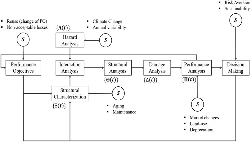
FIGURE 1. Proposed Performance-Based Coastal Engineering (PBCE) framework. The framework consists of six basic components: (1) performance objectives, (2) hazard analysis, (3) structural characterization, (4) structural analysis, (5) damage analysis, and (6) performance analysis.

Performance Objectives

Performance objectives (PO) are discrete qualitative measures of expected performance that are based on probable damages to the system given the occurrence of a hazard. Although similar nomenclature can be used across different civil engineering subfields to denote performance expectations, their definition and associated damage states vary significantly depending on the type of structure, construction material, and hazard. In the literature, performance objectives and damage classifications have been proposed for various types of coastal structures and hazards (Van De Lindt and Dao, 2009; Van De Lindt and Taggart, 2009; Ciampoli et al., 2011; Li et al., 2012; Massarra, 2012; Ataei and Padgett, 2013; Barbato et al., 2013; Attary et al., 2017; Emanuel, 2017; Park et al., 2017; Tomiczek et al., 2017; Baradaranshoraka et al., 2019; Xiong et al., 2019). PO are commonly associated with structural integrity, operational status, incurred losses, or serviceability requirements (Ciampoli et al., 2011; Barbato et al., 2013; American Society of Civil Engineers, 2017). Performance objectives can be evaluated by the damage of individual structural and nonstructural components (American Society of Civil Engineers, 2017) or the overall state of the structure in the aftermath of a hazard event (Barbato et al., 2013).

Hazard Analysis

The hazard analysis component starts with the probabilistic characterization of the vector of intensity parameters $\mathbf{\Lambda }$. Since coastal structures might be exposed to both single-hazard (e.g., extreme winds, flooding, tsunamis) and multi-hazard (e.g., hurricane induced storm surge, wind, and waves) scenarios, the vector of intensity parameters $\mathbf{\Lambda }$ is described as:

$\mathbf{\Lambda }=\left[ {\left\{{\mathbf{\Lambda }}^1\right\}}^{\mathrm{T}}, {\left\{{\mathbf{\Lambda }}^2\right\}}^{\mathrm{T}}, \cdots , {\left\{{\mathbf{\Lambda }}^m\right\}}^{\mathrm{T}}\right]{ }^{\mathrm{T}}(\mathrm{1a})$

${\left\{{\mathbf{\Lambda }}^i\right\}}^{\mathrm{T}}={\left[{\lambda }_1^i, {\lambda }_2^i, \cdots ,{\lambda }_n^i\right]}^{\mathrm{T}},i\in \left[1,m\right](\mathrm{1b})$

Where $m$ corresponds to the number of individual hazards (i.e., single hazards), and $n$ denotes the number of intensity parameters in the $i^{th}$ hazard. Each of the parameters composing the individual vectors of $\mathbf{\Lambda }$ are explicitly a function of time. For example, if for the $i^{t\text{h}}$ hazard ${\lambda }_1^i\to {\lambda }_1^i\left(t\right)$, then, ${\mathbf{\Lambda }}^i\to {\mathbf{\Lambda }}^i\left(t\right)$ and $\mathbf{\Lambda }\to \mathbf{\Lambda }\left(t\right)$. Nevertheless, for the sake of simplicity, the mathematical expressions for the vector parameters are represented in shorthand notation as in Eq. 1a and Eq. 1b for the following components of the framework.

To select a suitable set of intensity parameters, consideration should be given to the hazard models selected to describe the event (Barbato et al., 2013), as well as their efficiency and sufficiency for the particular case study (i.e. hazard models might need information not available/very difficult to estimate at the site, or might be irrelevant for the overall performance of the structure) (Barbato et al., 2013). Considering an elevated residential coastal structure subjected to both significant surge and wave loads as an example, the vector of intensity parameters would be comprised of flood hazard intensity parameters (Barbato et al., 2013) such as surge depth $S_d$, significant wave height $H_s$, and flow velocities $V_x$, $V_y$. Therefore, in this case:

$\mathbf{\Lambda }=\left[ {\left\{{\mathbf{\Lambda }}^1\right\}}^{\mathrm{T}}\right](\mathrm{2a})$

${\left\{{\mathbf{\Lambda }}^1\right\}}^{\mathrm{T}}={\left[S_d,H_s,V_x, V_y\right]}^{\mathrm{T}}(\mathrm{2b})$

If wind, rainfall, or other types of hazards are seen or expected to cause significant loading to the structure during a hurricane or storm event, their respective ${\left\{{\mathbf{\Lambda }}^i\right\}}^{\mathrm{T}}$ vectors can be added in Eq. 2. In a fully probabilistic hazard analysis, the output of this PBCE component could be depicted in the form of a hazard curve, characterizing the mean annual rate of exceedance of a particular intensity parameter from its marginal distribution, or $n$-dimensional hazard surface characterizing the rates of joint intensity parameter exceedance. While in the coastal engineering community these joint exceedances or associated joint probability distribution functions are often lacking for a vector of intensity parameters, recent studies have made progress in this direction (Günay and Mosalam, 2013; Jia and Taflanidis, 2013; Hallowell et al., 2018; Attary et al., 2019; Do et al., 2020; Nofal et al., 2020). The hazard analysis component can also be conducted using a scenario-based analysis by selecting a representative hazard (e.g., worst-expected hazard, a hazard with a specific return period) scenario of the region, which can be used for rapid-response analysis or when the computational demand of a fully probabilistic analysis cannot be afforded. For instance, synthetic storms such as FEMA 36 and FEMA 33 (Ebersole et al., 2017; Melby et al., 2017), which result in approximately 500- and 100-years storm surge events in the Houston-Galveston region (Ebersole et al., 2017), respectively, have been commonly adopted in the literature to conduct scenario-based risk analysis in the Texas coast (Ebersole et al., 2017).

Structural Characterization

The uncertainty associated with the mechanical and geometrical properties of the system is described through the vector of structural parameters $\mathbf{\Xi }$. In general terms, these parameters are the ones required to describe the stiffness, strength, and geometry of the individual structural elements and the overall structure, such as material properties (e.g., modulus of elasticity $E$, yielding strength $f_y$), depth and height of beams and columns, characterization of the substructure, among others. However, further consideration should be given to systems where fluid-structure or soil-structure interactions play a critical role in the response of the structure, and their respective parameters should also be included. For instance, during hurricane events, significant scour can occur in the foundation of elevated residential structures and bridges, which can add to the collapse of these structures (FEMA, 2009; Briaud, 2015; Kameshwar and Padgett, 2018), in which case, parameters related to the soil properties of the site should also be considered. Moreover, the landscape, surrounding structures, topological factors, and system connectivity, might also play an important role in the loading process and response of individual structures (Barbato et al., 2013; Hatzikyriakou et al., 2016; Attary et al., 2017). For instance, shielding and canalization effects have been seen to play a key role in the loading process of coastal buildings structures (Hu et al., 2016; Tomiczek et al., 2016; Winter, 2019). The vector of structural parameter is defined as:

$\mathbf{\Xi }=\left[ {\left\{{\mathbf{\Xi }}^1\right\}}^{\mathrm{T}}, {\left\{{\mathbf{\Xi }}^2\right\}}^{\mathrm{T}}, \cdots , {\left\{{\mathbf{\Xi }}^s\right\}}^{\mathrm{T}}\right]{ }^{\mathrm{T}}(\mathrm{3a})$

for systems with more than one structure, and as

${\left\{{\mathbf{\Xi }}^i\right\}}^{\mathrm{T}}=\left[{\xi }_1^i, {\xi }_2^i, \cdots ,{\xi }_p^i\right]{ }^{\mathrm{T}},i\in \left[1,s\right](\mathrm{3b})$

for single structures, where $s$ corresponds to the number of structures, and $p$ denotes the number of structural parameters in the $i^{th}$ structure. In the case of elevated residential coastal structures (ERCS), some of the variables that might be considered are elevation of the lowest horizontal member, the strength of the connections, stiffness of individual structural components, Reynolds number, undrained shear strength of the soil, distance to the coast, number of structures in the surroundings, the distance between structures, among others.

Structural Analysis

The structural analysis provides the probabilistic characterization of the system response through the vector $\mathbf{\Theta }$ of engineering demand parameters. These can be defined in terms of the response of individual structural elements (e.g., plastic rotations of beams and columns, element forces), non-structural elements (e.g., loss of roof panels, infiltration damage to floors), or the overall behavior of the structure (e.g., drifts, loss of foundation) (Barbato et al., 2013; Günay and Mosalam, 2013). To accommodate systems composed of more than one structure, the vector parameter $\mathbf{\Theta }$ is defined as:

$\mathbf{\Theta }=\left[ {\left\{{\mathbf{\Theta }}^1\right\}}^{\mathrm{T}}, {\left\{{\mathbf{\Theta }}^2\right\}}^{\mathrm{T}},\cdots ,{\left\{{\mathbf{\Theta }}^s\right\}}^{\mathrm{T}}\right]{ }^{\mathrm{T}}(\mathrm{4a})$

${\left\{{\mathbf{\Theta }}^i\right\}}^{\mathrm{T}}=\left[{\theta }_1^i,{\theta }_2^i,\cdots ,{\theta }_r^i\right]{ }^{\mathrm{T}},i\in \left[1,s\right](\mathrm{4b})$

where $s$ corresponds to the number of structures and $r$ corresponds to the number of engineering demand parameters for the $i^{th}$ structure. The vector ${\mathbf{\Theta }}^i$ can combine different types of engineering demand parameters depending on the components of the system and is frequently composed of their respective peak values (Günay and Mosalam, 2013). In the case of ERCS subjected to surge and wave loads typical engineering demand parameters include shear force at the connections, pier deformations, pressures on walls, or uplift pressure.

Damage Analysis

The damage analysis allows the quantification of the probability of exceeding a certain damage level of a given structural element or the overall structure conditioned on their respective engineering demand parameters (EDPs). The damage function is discretized using damage states, which describe the amount of damage that the element undergoes until its complete loss of functionality or collapse when subjected to different levels of intensity (i.e. different hazard scenarios, increment in the intensity parameters). To estimate the element damage, a limit state function $\mathit{g}$ is evaluated, where the capacity corresponding to each damage state is compared with the EDPs obtained from the structural analysis component. Recent efforts have been devoted to the probabilistic characterization of structural element capacities (Gardoni et al., 2002; Choe et al., 2008; Sharma et al., 2015), however, these can be defined as deterministic if the information on the variability of the capacity is not available, comes at a large computational cost, or is deemed relatively known. The vector of engineering capacity parameters (ECPs) is then defined as:

$\mathbf{\Psi }={\left[ {\left\{{\mathbf{\Psi }}^1\right\}}^{\mathrm{T}},{\left\{{\mathbf{\Psi }}^2\right\}}^{\mathrm{T}},\cdots ,{\left\{{\mathbf{\Psi }}^s\right\}}^{\mathrm{T}}\right]}^{\mathrm{T}}(\mathrm{5a})$

${\left\{{\mathbf{\Psi }}^i\right\}}^{\mathrm{T}}=\left[{\psi }_1^i,{\psi }_2^i,\cdots ,{\psi }_r^i\right],i\in \left[1,s\right](\mathrm{5b})$

where $s$ corresponds to the number of structures and $r$ corresponds to the number of ECPs for the $i^{th}$ structure. The limit state function for each damage state is defined as:

${\mathit{g}}_j^i={\theta }_j^i-{\psi }_j^i,i\in \left[1,s\right],j\in \left[1,r\right](6)$

This comparison allows defining if a certain component has failed using a Bernoulli random variable, which will state if the element has exceeded a certain damage level or not. Subsequently, the probabilistic characterization of the vector $\mathbf{\Delta }$ of damage parameters is given by:

$\mathbf{\Delta }={\left[{\left\{{\mathbf{\Delta }}^1\right\}}^{\mathrm{T}},{\left\{{\mathbf{\Delta }}^2\right\}}^{\mathrm{T}},\cdots ,{\left\{{\mathbf{\Delta }}^s\right\}}^{\mathrm{T}}\right]}^{\mathrm{T}}(\mathrm{7a})$

${\left\{{\mathbf{\Delta }}^i\right\}}^{\mathrm{T}}={\left[{\delta }_1^i,{\delta }_2^i,\cdots ,{\delta }_r^i\right]}^{\mathrm{T}},i\in \left[1,s\right](\mathrm{7b})$

where

$\begin{array}{l}{\delta }_j^i=1if{\theta }_j^i>{\psi }_j^i,i\in \left[1,s\right],j\in \left[1,r\right]\\ =0otherwise\end{array}(8)$

To consider the possibility of complete collapse or loss of functionality of the structure, the last parameter of the damage vector is reserved to account for a global parameter that can define global collapse:

$\begin{array}{l}{\delta }_r^i=1collapse\\ =0nocollapse\end{array}(9)$

This allows checking the global stability of the system before performing computationally expensive element-wize calculations (Günay and Mosalam, 2013). Moreover, the limit state function is also used to develop fragility models that depict the probability of reaching or exceeding a damage state given intensity parameters and/or structural parameters. If fragility functions are already available for individual structural elements or the structural system itself, the component of structural analysis can be avoided, and the probability of exceeding a certain damage state is directly evaluated from the fragility model. Multiple fragility functions have been proposed in the literature for diverse types of coastal systems, with a recent shift toward parameterized fragility models, where fragility functions are conditioned on specific structural characteristics and load conditions (Ataei and Padgett, 2013; Tomiczek et al., 2014; Hatzikyriakou et al., 2016; Balomenos and Padgett, 2018; Saeidpour et al., 2018; Bernier and Padgett, 2019). In the case of ECRS under surge and wave load, most of the fragility models to date have been empirically derived in the aftermath of major hurricane events (Hatzikyriakou et al., 2016; Tomiczek et al., 2014, 2017); with some recent efforts to develop parameterized fragility functions using numerical simulations (Do, 2016; Do et al., 2020). To incorporate cascading effects, the damage parameter of an individual structure or system ${\mathbf{\Delta }}^i$ is computed by factoring in the cascading parameter with its demand parameter in the limit state function. For instance, if structure two is subjected to waterborne debris load (e.g. cascading effect) coming from structure one, the limit state function of structure two becomes:

${\mathit{g}}_j^2={\beta }^1\cdot {\theta }_j^2-{\psi }_j^2,j\in \left[1,r\right](10)$

Where ${\beta }^1>1$ is the cascading parameter coming from the damage analysis of structure 1. Moreover, the shielding effect is incorporated by considering $\beta <1$.

Performance Analysis

The component of performance analysis computes the marginal probability distribution of the decision variable DV. The selection of the decision variable implies an active communication with the stakeholders to adopt metrics that adequately portray the desired/required performance objectives of the system. A common choice of DV includes the annual economic loss or the life-cycle cost of the structure—the reason why the computation of the marginal probability distribution of the decision variable is typically known as “loss analysis” (Porter, 2003; Ciampoli et al., 2011; Barbato et al., 2013; Günay and Mosalam, 2013; Attary et al., 2017). Nevertheless, decision variables encompass various aspects of importance for stakeholders and communities, that cover a wide selection of metrics such as downtime, injuries and fatalities (Jonkman, 2007; Günay and Mosalam, 2013), carbon footprint (Dehghani and Shafieezadeh, 2019; Padgett and Tapia, 2013), environmental impact, and the threat to public health in the event of failure (Reible et al., 2006), loss of community service, and even aspects related to psychological trauma after a hazard event. Indirect costs (e.g. loss of productivity in the community, cost of power outages (Bjarnadottir et al., 2018), a decline in revenue (Becker et al., 2015), unemployment, evacuation efforts (Whitehead, 2003) and intangible consequences (e.g. ecosystem damages (Becker et al., 2015), individuals’ well-being (Berlemann, 2016)) should also be considered since they have a great effect on the total cost and impact of natural disasters (Dong and Li, 2016). Moreover, the DV can also be defined as a system metric, where the result of individual building responses is used to estimate the system-level performance, as in the case of community resilience metrics (Lounis and McAllister, 2016; Kameshwar et al., 2019) or sustainable neighborhoods (Ju et al., 2016; Wangel et al., 2016).

In the case of economic losses, the probability of exceeding a certain loss can be estimated by assigning costs to the actions needed to repair or replace the structural elements depending on the sustained damages computed in the damage analysis component. The loss associated with downtime can be estimated by computing the incurred costs due to loss of functionality of the system [e.g. business interruption, loss of household production (Rose et al., 2007)]. Moreover, different studies have proposed methodologies to assess the value of life (Landefeld and Seskin, 1982; Jonkman, 2007; Ditlevsen and Friis-Hansen, 2009; Luechinger and Raschky, 2009; Kousky, 2014; Daniell et al., 2015; Yu and Tang, 2017), however, serious ethical questions arise when estimating the cost of fatalities or injury in the aftermath of natural disasters. CO₂ or other greenhouse gas emissions and embodied energy are typical DVs (Dehghani and Shafieezadeh, 2019; Lounis and McAllister, 2016; Müller et al., 2013; Padgett and Tapia, 2013) to measure the environmental impact of structures and infrastructure systems by associating costs to the emissions of the manufacturing process and transportation of construction materials (Lounis and McAllister, 2016), maintenance and repair (Dehghani and Shafieezadeh, 2019), and any detour of vehicles during the construction phase or in retrofitting, inspection, and repair actions (Lounis and McAllister, 2016; Padgett and Tapia, 2013). Furthermore, decision variables concerning public health, the individual’s well-being, and psychological impact can be associated with the expected number of failures of residences and special structures such as hospitals in a community in the aftermath of a hazard event. For instance, failure of residences during storm-surge events can release toxic substances into the environment in the form of construction debris, household-stored chemicals, fuel in flooded cars, and their improper disposal (Reible et al., 2006), jeopardizing the health of entire communities. Potentially more than one decision variable can be evaluated to analyze different consequences of system or element failure.

The vector $\mathbf{\Xi }$ representing the unit value of DV for each damageable element is expressed as:

$\left[\mathbf{\Xi }\right]=\left[\left[{\mathbf{\Xi }}^1\right],\left[{\mathbf{\Xi }}^{\mathbf{2}}\right],\cdots ,\left[{\mathbf{\Xi }}^s\right]\right](\mathrm{11a})$

$\left[{\mathbf{\Xi }}^i\right]=\left[\begin{array}{cccc}{\gamma }_1^{i,1}& {\gamma }_1^{i,2}& \cdots & {\gamma }_1^{i,u}\\ {\gamma }_2^{i,1}& {\gamma }_2^{i,2}& \cdots & {\gamma }_2^{i,u}\\ ⋮& ⋮& \ddots & ⋮\\ {\gamma }_r^{i,1}& {\gamma }_r^{i,2}& \cdots & {\gamma }_r^{i,u}\end{array}\right],{\mathbf{\Xi }}^i\in {ℝ}^{r\times u},i\in \left[1,s\right](\mathrm{11b})$

where

${\gamma }_k^{i,j}=unitvalueof{k}^{th}ECPofthe{i}^{th}structureforthe{j}^{th}DV$

and ${\gamma }_r^{i,u}$ represents the value associated with global collapse. Therefore, the value of each $u^{th}$ decision variable is given by:

$\mathbf{\Pi }={\left[{\left\{{\mathbf{\Pi }}^1\right\}}^{\mathrm{T}}, {\left\{{\mathbf{\Pi }}^2\right\}}^{\mathrm{T}},\cdots ,{\left\{{\mathbf{\Pi }}^s\right\}}^{\mathrm{T}}\right]}^{\mathrm{T}}(\mathrm{12a})$

${\left\{{\mathbf{\Pi }}^i\right\}}^{\mathrm{T}}={\left[{\pi }_1^i,{\pi }_2^i,\cdots ,{\pi }_u^i\right]}^{\mathrm{T}}(\mathrm{12b})$

where the $u^{th}$DV can stand for loss of life, money, embodied energy, CO₂ emissions, downtime, among others. Thus, ${\pi }_j^i$ stands for the total loss of the $i^{th}$ structure for the $j^{th}$DV:

${\pi }_j^i=\left(1-{\delta }_r^i\right){\displaystyle \sum _{j=1}^{j=r-1}{\gamma }_k^{i,j}{\delta }_k^i + {\gamma }_k^{i,j}{\delta }_r^i},i\in \left[1,s\right],k\in \left[1,u\right](\mathrm{12c})$

Therefore, for the case of community metrics

$\left\{ℂ\right\}=\left\{C_1,C_2,\cdots , C_u\right\}(\mathrm{13a})$

where

$C_j=Totalcommunitylevellossforthe{j}^{th}DV$

$C_j={\displaystyle \sum _{i=1}^s{\pi }_j^i}(\mathrm{13b})$

Time-Dependent Probabilistic Graphical Model

With the main components of the PBCE defined, a mathematical abstraction of this framework is pursued, first with an overview of the adopted model—a dynamic Bayesian network, followed by an example of how to construct a dynamic Bayesian network from the PBCE framework representation. Probabilistic graphical models, such as Bayesian and dynamic Bayesian networks, provide a flexible approach for model updating using evidence and have been successfully implemented in the assessment of civil structures and infrastructure systems (Bensi et al., 2013; Schultz and Smith, 2016; Khakzad and Van Gelder, 2018). Moreover, the basic construction of probabilistic graphical models using nodes and links, allows direct consideration of dependencies (links) between different random variables (nodes) (Bensi et al., 2013), providing not only an efficient sampling strategy but also the easy incorporation of engineering judgment in the model while facilitating communication with stakeholders. This section provides a general overview of Bayesian networks followed by the case of dynamic Bayesian networks. Subsequently, their relevance and adaptation to modeling the PBCE problem are described.

Bayesian Network

Bayesian networks (BN) are directed acyclic probabilistic graphical models that represent the joint probability density function $p\left(\mathbf{X}\right)$ of a set of random variables $\mathbf{X}$. The random variables are represented as nodes and the causal relationships among them are represented by links directed from the parent node to the children node. The causal relationship constitutes the conditional dependence of the child random variable to the parent random variable. A detailed description of BN can be found in Russel and Norvig (2002). Figure 2A illustrates a simple BN where nodes $\mathbf{X}=\left\{{\mathit{X}}_1,{\mathit{X}}_2,{\mathit{X}}_3,{\mathit{X}}_4,{\mathit{X}}_5\right\}$ represent the random variables of the model. In this case, $X_5$ is the child node of $X_3$, while $X_2$ and $X_3$ have $X_1$ as the parent node and $X_4$ as the child node. The joint probability density function of the network is evaluated as the product of individual conditional probabilities as:

$p\left(\mathbf{X}\right)=p\left({\mathit{X}}_1,{\mathit{X}}_2,{\mathit{X}}_3,{\mathit{X}}_4,{\mathit{X}}_5\right)=p\left({\mathit{X}}_1\right) p\left({\mathit{X}}_2|{\mathit{X}}_1\right)p\left({\mathit{X}}_3|{\mathit{X}}_1\right)p\left({\mathit{X}}_4|{\mathit{X}}_2,{\mathit{X}}_3\right)p\left({\mathit{X}}_5|{\mathit{X}}_3\right)(14)$

The marginal probability density function (pdf) of any random variable is computed by performing integration of the joint pdf over the remaining random variables. For example

$p\left(X_4\right)={\displaystyle \underset{{\Omega }_{X_1}}{\int }{\displaystyle \underset{{\Omega }_{X_2}}{\int }{\displaystyle \underset{{\Omega }_{X_3}}{\int }p\left(X_4|X_2,X_3\right)p\left(X_2|X_1\right)p\left(X_3|X_1\right)d{X}_{3}d{X}_{2}d{X}_1}}}(15)$

where ${\text{Ω}}_{X_1}$, ${\text{Ω}}_{X_2}$, and ${\text{Ω}}_{X_3}$ are the domains of the random variables $X_1, X_2,$ and $X_3$, respectively. In the event of the availability of information related to any random variable in the model, BN offers the potential to update the probabilities in the network. BN propagates the evidence throughout the network to update the probability distributions of all the other variables following Bayes’ theorem. For example, if evidence $e$ is observed for the random variable $X_2$, the marginal pdf of $X_3$ is updated as follows

$p\left(X_3|e\right)=\frac{p\left(X_3,e\right)}{p\left(e\right)}=\frac{{\displaystyle {\int }_{{\Omega }_{X_1}}{\displaystyle {\int }_{{\Omega }_{X_2}}p\left(X_3|X_1\right)p\left(e|X_2\right)p\left(X_2|X_1\right)d{X}_{2}d{X}_1}}}{{\displaystyle {\int }_{{\Omega }_{X_1}}{\displaystyle {\int }_{{\Omega }_{X_2}}p\left(e|X_2\right)p\left(X_2|X_1\right)d{X}_{3}d{X}_{2}d{X}_1}}}(16)$

FIGURE 2

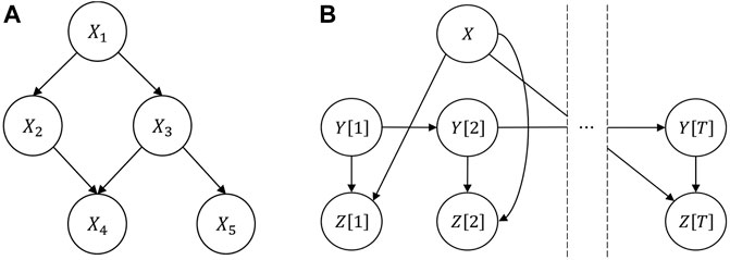
FIGURE 2. (A) Basic example of a Bayesian network. Nodes $\mathbf{X}=\left\{X_1,X_2,X_3,X_4,X_5\right\}$ represent the random variables of the model. $X_5$ is the child node of $X_3$, $X_2$ and $X_3$ have $X_1$ as the parent node, and $X_4$ as the child node (B) Example of a Dynamic Bayesian Network (DBN). The DBN network models the probabilities of the random variables $Y\left[t\right]$ and $Z\left[t\right]$ as it evolves discretely over each time instant $t\in \left\{\mathrm{1,2},\cdots ,T\right\}$.

Dynamic Bayesian Network

A Dynamic Bayesian Network (DBN) is an extension of classical BN which is capable of modeling the uncertainties of discrete time-varying systems (Murphy and Russell, 2002). Figure 2B shows an example of a DBN that models the probabilities of the set of random variables $Y\left[t\right]=\left\{Y\left[1\right],Y\left[2\right],\cdots ,Y\left[T\right]\right\}$ and $Z\left[t\right]=\left\{Z\left[1\right],Z\left[2\right],\cdots ,Z\left[T\right]\right\}$ as they evolve discretely over each time index $t\in \left\{\mathrm{1,2},\cdots ,T\right\}$. The joint pdf of the network is evaluated as the product of the individual conditional pdf of the variables in the network as in BN (Straub, 2009)

$p\left(X,Y\left[t\right],Z\left[t\right]\right)={\displaystyle \prod _{t=1}^{T}p\left(Z\left[t\right]|Y\left[t\right],X\right)}(17)$

where $X$ is a time-invariant random variable. Therefore, given the availability of evidence regarding any node, the probabilities of each random variable would be updated according to Bayes’ theorem as illustrated for BN.

For both BN and DBN, the child node originates from one or more parent nodes which are modeled through a directed arrow. The nodes that share a child node but are not children of that node are spouse nodes. The parent, child, and spouse nodes, together, form a Markov blanket. Apart from the nodes within the Markov blanket of a node, that random variable is independent of all other variables present in the network. The efficient sampling and inference of the joint pdf of the network are attributed to this concept of d-separation (Markov blanket) of a node in the network (Pearl, 2014). As new evidence of any node becomes available, the joint pdf of the network gets updated following the Bayes’ theorem, and the posterior distribution of the random variables that are inside the Markov blanket of the observed random variable gets updated. However, the marginal pdfs of those random variables that are d-separated from the observed node do not change. It is noteworthy to mention, that in the context of BNs and DBNs, evidence constitutes any measurement associated with one or more of the random variables in the network. New models or forecasts of the relations between the random variables (links) can be incorporated, but this would imply the modification of the network and a new model.

Dynamic Bayesian Network Modeling of the Performance-Based Coastal Engineering Framework

One of the key features of the proposed PBCE framework is its adaptability to model time-varying systems through the incorporation of time-varying parameters into the description of each of the components presented in Components of the Performance-Based Coastal Engineering Framework. DBNs offer the capability of modeling discrete-time or space varying systems and allow to represent stochastic processes by constructing a BN over each discrete point in time (Straub, 2009). To model the flow of information from one discrete-time index $t$ to the following time index $t+1$, one or more nodes of the BN at time $t$ are connected through directed links to nodes in the BN at time $t+1$ (Ghahramani, 1997; Straub, 2009), as seen in Figure 2B by the link connecting $Y\left[1\right]$ to $Y\left[2\right]$. For illustration purposes, we use a typical Gulf Coast elevated residential structure subjected to storm surge and wave loading to portray how to construct a discrete in time DBN model from the formulation of the PBCE framework. The selected house is a typical wood-frame structure elevated on piles that was constructed in the year 2000 (Fereshtehnejad et al., 2021). Figure 3A shows the complete PBCE framework for this example, defined both as continuous and discrete (i.e., at a time index $\left[i\right]$) in time. Since the objective of this section is to show the basic construction of a DBN from the vectors of parameters of the PBCE framework, herein we focus on the definition of nodes and links starting from the description of the parameters relevant to the case study. The details on the mathematical description of the links and how each vector is constructed along with the probabilistic description of its parameters can be found in the following section (Realistic System: Existing Elevated Residential Structure).

FIGURE 3

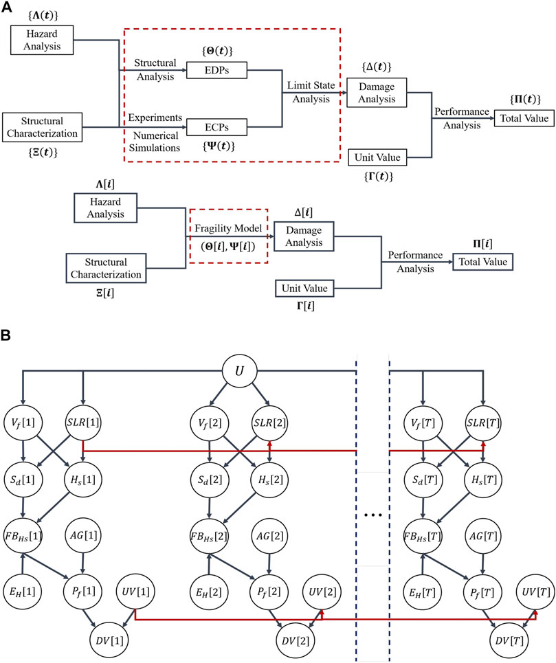
FIGURE 3. (A) Performance-Based Coastal Engineering framework representation of a typical Gulf Coast elevated residential structure subjected to storm surge and wave loading, defined both as continuous and discrete (i.e., at a time index $\left[i\right]$) in time (B) DBN model of a typical Gulf Coast elevated residential structure subjected to storm surge and wave loading.

In this case study, the intensity parameters are selected as the significant wave height $H_s$ and the surge depth $S_d$ at the location of the structure, which is defined based on two hazard parameters (i.e., parameters concerning the hazard itself or variables necessary for the numerical simulation of the hazard), the forward velocity of the storm $V_f$ and the sea-level rise ($SLR$). As mentioned in the component of damage analysis in the previous section, if fragility models are available for the region, structural elements, or the structure itself, these can be used to evaluate the damage based on the hazard and the structural characterization components. The variant number five of the fragility models proposed by Tomiczek et al. (2014) is used to define the probability of failure $P_f$ of the house, which is a function of the significant wave height $H_s$, the free-board height (i.e., the free distance between the crest of the wave and the lowest horizontal structural member of the house), and the year of construction (categorized by age groups). The free-board height ($F{B}_{Hs}$) is itself a function of $H_s$, $S_d$, and the height of the house with respect to the ground $E_H$. Therefore, the vector of structural parameters consists of both $E_H$ and the age of the house ($AG$). The unit value ($UV$) corresponds to the one associated with global collapse of the house (i.e., ${\gamma }_r^{i,u}$) and is defined as the replacement cost of the house. Finally, the decision variable DV is set as the probable economic loss of the structure based on its structural damage (i.e., unit value scaled with the probability of failure of the house).

With the nodes and their basic dependencies (links) defined, the DBN can be constructed by replicating the basic BN structure at each time step and connecting the nodes that have a time-variant relation. Figure 3B shows the DNB constructed for the house, where it is assumed that the time variation of the sea-level rise and the unit value of the replacement cost of the house are represented with the aid of a mathematical expression. For illustration, the probability distribution of the hazard parameters is assumed to be conditioned on a random influencing variable $U$, to account for possible common influencing factors (e.g. hazard model, climate change simulations, statistical uncertainties) (Straub and Der Kiureghian, 2010). Moreover, and as can be depicted in Figure 3B, given the multiple parameters that play a role in defining a PBCE framework analysis, the constructed DBNs will turn out to be very large, and even more when modeling systems with multiple structures. Methods have been proposed to significantly reduce the computational cost of large BN networks (Bensi et al., 2013). However, it is still challenging to perform exact inference of the network’s joint pdf because it depends on the nature of the individual probability distribution of the variables. Closed-form solutions exist for DBNs composed solely of discrete or Gaussian random variables (Straub, 2009; Shenoy, 2012; Lerner et al., 2013). In most applications related to coastal engineering, the parameters are defined by a combination of discrete and continuous random variables, each one with a different probability distribution. This makes the computation of the integrals needed to estimate the full posterior distribution of the random variables an impossible task.

To handle these situations, approximate inference algorithms such as Markov Chain Monte Carlo (MCMC) are used to avoid the exact computation of integrals by estimating the posterior distribution using ergodic averages (Yildirim, 2012). The Gibbs sampling algorithm is an MCMC technique that allows the efficient computation of large BNs, in which the Monte Carlo estimates of the marginal pdfs of each node are obtained by generating samples from a Markov chain. In this way, the explicit computation or inversion of the joint pdf is averted to generate samples from a complex marginal pdf. This is done by generating samples of the posterior distribution of a random variable in its conditional distribution form (as presented in Eq. 14 and Eq. 17) while maintaining the other random variables fixed until convergence. This is repeated for all the random variables in the BN. Nevertheless, convergence to the true joint probability distribution is only ensured for a large number of samples (i.e., when we reach the stationary state), which means that the early random samples might not be representative of it. Therefore, these initial samples are usually discarded, known as the tuning process or bur-in period (Yildirim, 2012). Details on the Gibbs sampling strategy can be found in (Yildirim, 2012). In this study, Markov chain Monte Carlo simulation with Gibbs sampling is applied. OpenBUGS (Spiegelhalter et al., 2007), an open-source Bayesian inference software, is used to implement the DBN model for the case studies discussed in the subsequent section. According to the best knowledge of the authors, this is the first instance of DBN adaptation to model a time-dependent PBE framework. Although this paper focuses on the PBCE framework, modeling concepts of DBN are easily transferable to other PBE frameworks.

Illustrative Case Studies

In this section, two case studies are introduced to illustrate the application of the PBCE framework and highlight two of its key features, the incorporation of time-varying parameters and cascading effects. First, the DBN constructed for the elevated residential structure in Dynamic Bayesian Network Modeling of the Performance-Based Coastal Engineering Framework (Figure 3B) is used to evaluate the probable economic loss associated with the replacement cost of the house (DV) under surge and wave loading. However, due to a lack of information on the year-to-year time variation of the parameters in the DBN model of the house, the marginal probability of the DV is computed independently for the years 2030, 2050, and 2100, by evaluating their respective BNs. For each year, the dependencies of the parameters and their mathematical description are elaborated to compute the marginal probability distribution of the economic loss given that a storm characteristic of the hazard conditions of that year occurs. The second case study corresponds to a system of two frames where the applicability of the framework to model cascading effects and time-varying systems is showcased. The year-to-year variation of relevant parameters in the model is included and the DBN evaluated for an illustrative period of analysis. In both examples, the evidence is incorporated into the model to demonstrate its effect in the estimates of the decision variable and highlight the flexibility of the framework to integrate new information in the model as it becomes available.

Realistic System: Existing Elevated Residential Structure

The residential building stock is one of the most vulnerable systems to hurricane hazard, and in a general sense, it dictates the overall impact of a storm in a community being a key component of the response before and after the hazard. Herein, a representative Gulf Coast wood-frame house is used to showcase the potential impact of storm surge and wave loading in the residential building stock when considering time-varying factors such as climate change and structural degradation. The house is selected randomly from a building inventory from Galveston Island, Texas (Fereshtehnejad et al., 2021). This database contains information on more than 15,000 structures and features such as geographical coordinates, year of construction, the elevation of the house with respect to the ground, and socio-demographical data (Fereshtehnejad et al., 2021). As mentioned in Dynamic Bayesian Network Modeling of the Performance-Based Coastal Engineering Framework, the house is elevated on piles, with a 4.572 m (15 ft) elevation above ground and was constructed in the year 2000. In general, coastal residential structures are designed to avoid the effects of surge and waves, which in turn makes the failure probability models highly sensitive to the free-board height. To better capture this effect, a lognormal distribution $E_H\sim LN\left(4.572m,0.023m\right)$ is used to define the elevation of the house, with the mean value set to the database reported elevation (15 ft) and a standard deviation of 0.023 m (0.25 ft) to consider the uncertainty associated with measurement error.

Hazard Analysis

Galveston Island is located in a hurricane-prone region susceptible to the effects of storm surge and wave loading (FEMA, 2009; Liu and Irish, 2019). To consider the effect of a changing climate on the impact of future storms, the forward velocity of the storm $V_f$ and projected increments in the local sea-level are considered, given their influence on surge generation during hurricane events (Liu and Irish, 2019; Moon et al., 2019; Ebad Sichani et al., 2020; Hassanzadeh et al., 2020). In this study, synthetic variations of the scenario storm FEMA 33 (FEMA, 2013; Ebersole et al., 2017) are used to define the hazard as an illustration of the framework. However, in the future, fully probabilistic hazard analysis under climate change conditions should be incorporated. Storm FEMA 33 is a synthetic storm that results in still-water elevations equivalent to approximately a 100-years return period storm in the Houston-Galveston region per (Ebersole et al., 2017; Melby et al., 2017). The reader can refer to (Ebad Sichani et al., 2020) for details on the hazard model and its outcomes which are adopted in this study. The physics-based numerical model ADCIRC + SWAN was implemented to simulate 19 synthetic variations of storm FEMA 33 by varying the forward velocity of the storm while keeping the spatial characteristics constant (Ebad Sichani et al., 2020). The model implements the TX2008 mesh [Federal Emergency Management Agency (FEMA) and U.S. Army Corps of Engineers (USACE), 2011] and comprises 2,500,861 triangular elements and 1,258,550 nodes. The mesh includes all the floodplains in Coastal Texas and has a high level of resolution in this area, with nodal spacing of approximately 30 m (100 ft) in the most refined areas. The geometry, bathymetry, and topography are representative of post-Ike conditions. Moreover, three sea-level rise (SLR) scenarios are considered: 20, 96.5, and 173 cm, which correspond to the minimum, average, and maximum value of the projected local-sea levels for Galveston between 2030 and 2100 (Kopp et al., 2014). The storm response parameters considered herein are the significant wave height $H_s$ and the surge depth $S_d$, which are selected based on existing fragility models for the region (Tomiczek et al., 2014). Therefore, the vector of intensity parameters $\mathbf{\Lambda }$ for the structure under analysis is defined as $\mathbf{\Lambda }=\left[ {\left\{{\mathbf{\Lambda }}^1\right\}}^{\mathrm{T}}\right]={\left[S_d,H_s\right]}^{\mathrm{T}}$.

To parameterize the intensity parameters for the specific location of interest, a regression model is developed for both significant wave height and surge depth as a function of the hazard parameters, the storm forward velocity, and sea-level rise. The polynomial model with third-order in $V_f$ and linear in $SLR$ is selected among other polynomial models using the Akaike information criterion (AIC) and the Bayesian information criterion (BIC). Eq. 18a and Eq. 18b shows the general form of the polynomial regression models adopted to predict both the surge depth and significant wave height for the house location

$S_d\left(V_f,SLR\right)=a_1+a_2\cdot V_f+a_3\cdot SLR+a_4\cdot V_f^2+a_5\cdot V_f\cdot SLR+a_6\cdot V_f^3+a_7\cdot V_f^2\cdot SLR(\mathrm{18a})$

$H_s\left(V_f,SLR\right)=b_1+b_2\cdot V_f+b_3\cdot SLR+b_4\cdot V_f^2+b_5\cdot V_f\cdot SLR+b_6\cdot V_f^3+b_7\cdot V_f^2\cdot SLR(\mathrm{18b})$

where $a_1,a_2,\cdots ,a_7$ and $b_1,b_2,\cdots ,b_7$ are the regression model coefficients presented in Table 1 along with their respective 95% confidence bounds. The regression models have an $R^2$ of 0.9980 and 0.9985, for surge depth and significant wave height, respectively.

TABLE 1

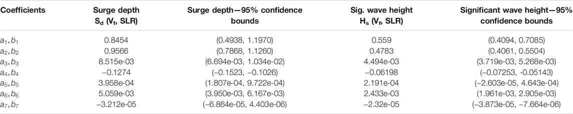
TABLE 1. Coefficients of the polynomial regression model and 95% confidence bounds for surge depth and significant wave height.

Sea-level rise projections and expected changes in the forward velocity of tropical cyclones are considered for three different years: 2030, 2050, and 2100. For each year, the local sea-level projections for Galveston proposed by Kopp et al. (2014) are used to define a normal distribution $SLR\sim N\left(\mu ,\sigma \right)$ of sea-level rise under three Representative Concentration Pathways (RCPs) (Meinshausen et al., 2011): 8.5, 4.5, and 2.6, which are defined to have an equal probability of occurrence. These RCP scenarios, which can be translated into the common influencing variable $U$ in Figure 3B, are associated with greenhouse gas emissions and represent a business-as-usual emissions scenario, a moderate mitigation scenario, and a strong mitigation policy scenario, respectively (Kopp et al., 2014). For further details on the local sea-level projections, the reader is directed to (Kopp et al., 2014). Table 2 presents the parameters of the normal distribution for each combination of year and RCP level. The standard deviation of the distribution is computed based on the 95% confidence bounds provided in (Kopp et al., 2014), while the mean is taken directly from the 50 percentile. The forward velocity of the storm is defined based on the range proposed by Liu and Irish (2019) for the Galveston region. Given the high uncertainty in the effects of climate change in the forward velocity of tropical cyclones (Ebad Sichani et al., 2020), a uniform distribution$V_f\sim U\left(\mathrm{3,12}\right)$ m/s is adopted in this case study.

TABLE 2

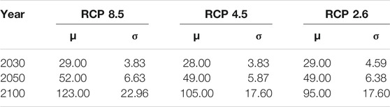
TABLE 2. Parameters of the normal distribution models for sea-level rise projections in Galveston, TX.

Structural Characterization, Structural Analysis, and Damage Analysis

The empirical fragility model proposed by Tomiczek et al. (2014) for wood-framed residences in the Galveston area following Hurricane Ike is used in this study to predict the probability of collapse (i.e. severe damage state) of the representative case study structure. Although the adopted fragility model has noted limitations, it also has the advantages of being representative of the construction practices of the region and developed for a tropical cyclone with predominant surge and wave loading effects (FEMA, 2009). The fragility model variant number five presented in (Tomiczek et al., 2014) is adopted in this study, which is a function of significant wave height $H_s$, free-board height $F{B}_{Hs}$, and age group $AG$. The free-board height represents the free distance between the lowest-horizontal member of the structure and the crest of the wave (i.e. negative values representing the waves reaching the structure), while the age group represents the age of the structure and construction practices (e.g. pre-1974, 1974–1987, 1987–1995, 1995–2008) (Tomiczek et al., 2014). Eq. 19 presents the fragility model proposed in (Tomiczek et al., 2014).

$P_F^{Fr}=\{\begin{array}{c}\Phi \left(-3.56+1.52H_s-1.73H_s\times F{B}_{Hs}-0.31F{B}_{Hs}^2-0.141A{G}^2\right)F{B}_{Hs}\ge -2.79H_s\\ \Phi \left(-3.56+1.52H_s+2.42H_s^2-0.141A{G}^2\right),F{B}_{Hs}<-2.79H_s \end{array}(19)$

where $\Phi$ is the Gaussian cumulative distribution function. Therefore, the vector of structural parameters $\mathbf{\Xi }$ is defined as $\mathbf{\Xi }=\left[ {\left\{{\mathbf{\Xi }}^1\right\}}^{\mathrm{T}}\right]={\left[E_H,AG\right]}^{\mathrm{T}}$, where $E_H$ is the elevation of the house in meters (with respect to the ground) necessary to compute the free-board height $F{B}_{Hs}$. Given that an existing fragility model is available for estimating the failure probability of the structure, the explicit definition of the vectors of engineering demand $\mathbf{\Theta }$ and capacity $\mathbf{\Psi }$ parameters, as well as the damage measures $\mathbf{\Delta }$ is averted. The case study residence was constructed in the year 2000, thus, according to the age groups proposed, $AG=4$. And, as mentioned in the description of the case study, $E_H\sim LN\left(4.572m,0.023m\right)$.

To capture the degradation of the structure over time, a reduction factor $R$ is applied to the fragility model (Bjarnadottir et al., 2011). Values of $R=-15\%$ (Nakajima and Murakami, 2010), $R=-25\%$ (Cavalli et al., 2016), and $R=-55\%$ (Crews et al., 2008) are selected for the years 2030, 2050, and 2100, respectively. These values are based on experimental studies on the degradation of the mechanical properties of different wood specimens and structural timber from the literature, where the changes in flexural strength (i.e., modulus of rupture) and stiffness (i.e., modulus of elasticity) from salvaged timber and new timber are compared.

Eq. 20 shows the modified fragility function. The strengthening of the structure is represented by considering positive values of R (Bjarnadottir et al., 2011).

$p_f=P_F^{Fr}\cdot \left(\frac{100-R}{100}\right)(20)$

Performance Analysis

As mentioned in Dynamic Bayesian Network Modeling of the Performance-Based Coastal Engineering Framework, the unit value UV is defined as the replacement cost of the structure $C$$\left(\left[{\mathbf{\Xi }}^i\right]=\left[ {\gamma }_r^{i,u}\right]=C\right)$. To compare the incurred cost of replacing the house in the three years of analysis (2030, 2050, and 2100), the replacement cost is computed in present value (PV) in dollars and then projected to the respective future value (FV). The FV considers the increase in the value of money over time by applying an interest rate that allows forecasting the value of a present amount of money in the future (Carther, 2020; Chen, 2020). Thus, the incurred cost of replacing the structure in the future (2030, 2050, and 2100) is estimated. The FV of the replacement cost is defined as (Carther, 2020; Chen, 2020)

$U{V}_t=C\cdot {\left(1+i_t\right)}^{N-1}(21)$

where $U{V}_t$ is the unit value in the year $t$, $C$ is the unit value in the year 2020, $i_t$ is the interest rate per year, and $N$ is the number of time periods (years) starting from the year 2020. For instance

$U{V}_{2030}=C\cdot {\left(1+i_t\right)}^{10-1}(22)$

The replacement cost of the structure in the present (2020) value dollars is estimated as $C=\text{\$}\mathrm{448,}\text{400}$, using typical square foot costs for a two-story wood-frame residence in Galveston, TX (Gordian, 2019). The interest rate is assumed as $i_t=3\%$ (based on inflation rate (Li and Ellingwood, 2009)), and $N=10$, $N=30$, and $N=80$, for the years 2030, 2050, and 2100, respectively.

The decision variable DV is selected as the expected economic loss in case of failure given the occurrence of a hurricane in the year under analysis (2030, 2050, and 2100, in this case study). Therefore, for a given year,

$\Pi =\left[ {\left\{{\mathbf{\Pi }}^1\right\}}^{\mathbf{T}}\right]=L_t(\mathrm{23a})$

$L_t=p_f\cdot U{V}_t(\mathrm{23b})$

where $L_t$ is the expected loss in the year $t$ based on the structural damage suffered by the house in the same year. The decision variable (DV) considered for the case study is the loss $L_t$associated with the replacement of the structure.

Results and Discussion

OpenBUGS (Spiegelhalter et al., 2007) is used to implement the BN models of the 3 years of analysis. The convergence of Markov chain Monte Carlo (MCMC) simulation is ensured by computing the Gelman-Rubin statistic $\widehat{R}$ (Gelman and Rubin, 1992) corresponding to various starting iteration steps (Figure 4A). Five MCMC chains are used to draw 250,000 samples from the target stationary posterior distribution. These 250,000 samples are obtained after the tunning process (burn-in period) to ensure the convergence to the true posterior distribution. Here, 10,000 iterations were discarded in the burn-in period. Figures 5A–C presents the normalized histogram of failure probability of the house $p_f$ for the years 2030, 2050, and 2100, respectively. The bounded distribution is heavily skewed about 0 (no failure) for the years 2030 and 2050, and about one (total failure) for the year 2100, which is explained by the high sensitivity of the failure probability to the flood line reaching the structure. Given that the forecast values of $SLR$ are significantly larger for the year 2100 compared to the years 2030 and 2050 for all three RCP levels (Table 2), it is more probable that the flood line surpasses the height of the lowest horizontal member of the house, creating a big skewness toward complete failure. With a similar argument, the lower values of flood depth for the years 2030 and 2050, ensure almost complete survival of the structure. Furthermore, the probability of exceedance of the loss ($L_t$) for the scenario event significantly goes up over time as observed in Figure 6. That can be attributed to the increased vulnerability of the structure as it ages and deteriorates as well as the influence of more severe climate conditions on the hazard intensity at the site of the structure. It is important to mention, that for the year 2100, the expected loss is bounded by the future value of the replacement cost of the structure in that same year (i.e., $L_t$ at the year 2100 assuming a 100% failure probability). By Figure 6, it is seen that in the year 2100, this threshold is first reached at a 50% probability of exceedance, which means that there is a 50% chance of exceeding a loss equivalent to $4,000,000 if a hurricane occurs in that year. Therefore, it is clear that given the assumptions of this study, the house is neither safe nor economically viable for climate conditions in the year 2100. Moreover, if we evaluate the incurred loss for a 100-years return period event (0.01 probability of exceedance), which is typical guidance for homeowners to elevate their houses (Federal Emergency Management Agency (FEMA), 2011; Work et al., 1999), the incurred loss would be equivalent to $20,000 in the year 2030 and $120,000 in the year 2050, that is equivalent to a 3.5 and 12% of the replacement cost of the structure at the given year, respectively. Then, under the conditions assumed in this study, the house would be deemed structurally safe up to the year 2050.

FIGURE 4

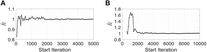
FIGURE 4. The convergence of MCMC simulation is ensured by computing the Gelman-Rubin statistic $\widehat{R}$ (Gelman and Rubin, 1992) corresponding to various starting iteration steps (A) the MCMC samples converge to the target stationary distribution after 5,000 samples (B) the MCMC samples beyond the initial 5,000 samples converge to the target stationary distribution.

FIGURE 5

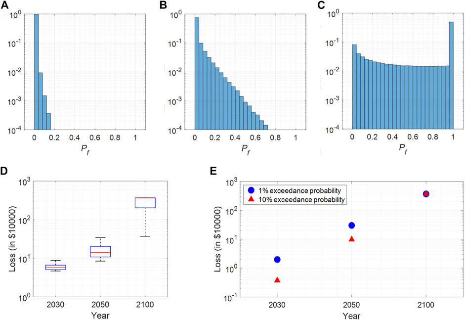
FIGURE 5. (A) The normalized histogram of failure probability of the house in the year 2030, (B) 2050, and (C) 2100, (D) the boxplot of the conditional distribution of loss given the probability of failure is more than 10%. The blue box limits the 25 and 75 percentile loss, the red line denotes the median loss, and the two end whiskers denote 5 and 95 percentile loss (E) the marginal loss corresponding to 1 and 10% exceedance probability for the years 2030, 2050 and 2100.

FIGURE 6

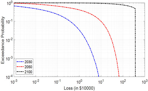
FIGURE 6. The variation of exceedance probability corresponding to the loss for the years 2030, 2050, and 2100.

Figure 5D shows the boxplot of the conditional distribution of loss $L_t$ given that the probability of failure is more than 10%. We can see that for the year 2100, the loss is highly dispersed and skewed, with a short upper distribution tail compared to the years 2030 and 2050, as expected due to the increasing uncertainty in time of climate projections. The dispersion of the loss for the years 2030 and 2050 is less, with a more extended upper tail in comparison to the conditional distribution of the loss in the year 2100. This can be explained by the fact that is less probable to have a high probability of failure of the house in these years, and therefore, the incurred loss will be less. In Figure 5E we compare the marginal loss corresponding to 1 and 10% exceedance probability for the years 2030, 2050, and 2100. It is apparent that the effect of exceedance probability in increasing the incurred loss becomes less prominent over the years. This can be seen by the reducing distance between the 1 and 10% exceedance probability from 2030 to 2100. This is consistent with Figure 6 where it is seen that the variation of exceedance probability with loss becomes steeper at higher values of probability of exceedance for all 3 years. Moreover, as mentioned previously, the incurred loss for the year 2100 reaches an upper bound at an exceedance probability of 50%, which explains that the loss is the same for both 1 and 10% probability of exceedance in Figure 5E.

To illustrate the incorporation of evidence in the PBCE framework for the residential structure, the influence of new knowledge on the loss estimates is evaluated. Specifically, evidence related to measurements of the elevation of the house $E_H$, storm forward velocity $V_f$, and evidence of the sea level rise $SLR$ are all considered. It is considered that this evidence is received in the year of analysis (2030, 2050, or 2100) and correspondingly modifies the results of the BN of that year. The computed 40,000 MCMC samples satisfactorily approximate the probability distribution of the loss. Figure 7A depicts the variation of the prior and the posterior (i.e., marginal distribution of the loss including evidence) exceedance probability corresponding to the loss $L_t$ for the year 2030. For this year, the evidence needed to compute the posterior distribution of the normalized future loss $L_t$ is given by $E_H=15ft$ with $CO{V}_{E_H}=0.5\%$ of measurement error, $V_f=6m/s$ with $CO{V}_{V_f}=15.0\%$, and $SLR=29cm$ with $CO{V}_{SLR}=3.0\%$. The coefficient of variation of the measurement error of the variables is assumed to depend on the precision of the measurement or the measuring instrument. For instance, it is expected in practice that the measurement of the elevation of the house with respect to the ground to be more precise in comparison to measurements of storm forward velocity. The sensitivity of the results to the variance of the measurement error will be assessed in future studies. As previously mentioned, the distribution of the probability of failure for the year 2030 is heavily skewed toward the no-failure scenario. Therefore, for this example, we compute the marginal distribution of the loss conditioned on the probability of failure being more than 0.1% to focus on the instances of non-zero loss. From Figures 7A,B it is apparent that the variability of the posterior probability of exceedance of the loss $L_t$ reduces in comparison to the prior distribution due to the incorporation of the observed evidence and its characterization.

FIGURE 7

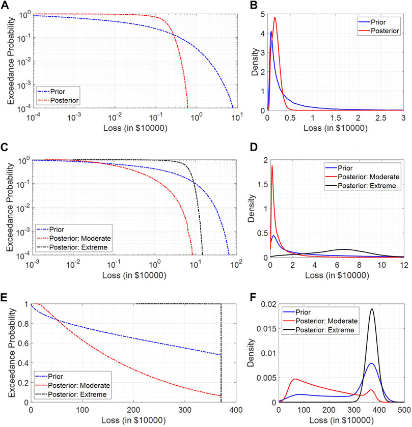
FIGURE 7. (A) The variation of the prior and the posterior exceedance probability corresponding to the loss for the year 2030 (B) the prior and the updated conditional posterior distribution of loss given probability of failure is more than 0.1% for the year 2030, (C) variation of the prior and the posterior exceedance probability corresponding to the loss under the observation of two different climate scenarios (moderate and extreme), for the year 2050, (D) the prior and the updated conditional posterior distribution of loss given probability of failure is more than 0.1% under the observation of two different climate scenarios (moderate and extreme), for the year 2050, (E) the variation of the prior and the posterior exceedance probability corresponding to the loss under the observation of two different climate scenarios (moderate and extreme), for the year 2100, (F) the prior and the updated conditional posterior distribution of loss given probability of failure is more than 10% under the observation of two different climate scenarios (moderate and extreme), for the year 2100.

For the years 2050 and 2100, we consider two climate scenarios, a moderate one where $V_f=9m/s$, and an extreme case where $V_f=6m/s$. The value of sea-level rise is selected as the mean of the $SLR$ distribution of the RCP scenarios of 8.5 and 2.6, for the moderate and extreme climate scenarios, respectively (Table 2). Therefore, in the moderate scenario, $SL{R}_{2050}=49cm$, and $SL{R}_{2100}=95cm$. Similarly, in the extreme climate scenario, $SL{R}_{2050}=52cm$, and $SL{R}_{2100}=123cm$. In both cases, $E_H=15ft$, $CO{V}_{E_H}=0.5\%$, $CO{V}_{V_f}=15.0\%$, and $CO{V}_{SLR}=3.0\%$. Figure 7C shows the variation of the prior and the posterior loss exceedance probability corresponding to the observation of two different climate scenarios (moderate and extreme), for the year 2050 given that the probability of failure is more than 0.1%. The posterior exceedance probability of the loss $L_t$ for both scenarios have a reduced variance compared to the prior distribution of the loss. Moreover, the incurred losses are more in the extreme weather climate scenario than that of the moderate scenario. In Figure 7D, we can see how the marginal distribution of the loss changes its mean from low values of loss (approximately $1,500) for the prior and moderate climate scenario, to higher losses in the extreme climate scenario (around $70,000). This is expected since the $SLR$ is higher for the extreme climate scenario, which in turn creates higher values of both surge depth and wave height, increasing the probability of failure of the house and the incurred loss. In Figure 8 the effect of different sets of evidence (moderate vs. extreme climate scenario) in the marginal posterior distribution of the loss is compared for the year 2050. It is seen how the more extreme climate conditions (expressed in terms of storm forward velocity and sea-level rise), change the shape and mass of the distribution of surge depth and wave height toward higher values (i.e., it is more probable to have high values of surge depth and wave height compared to the moderate climate and prior scenario), which leads to the increment of the probability of failure and incurred loss. Similarly, for the year 2100, Figure 7E shows how the probability of exceedance of the loss given that the probability of failure is more than 10%, nears one for most values of loss until it reaches the maximum loss (i.e., the future value of the replacement cost of the house in the year 2100). Moreover, as seen in Figure 7F, the more severe climate conditions, not only increases the losses but also makes high values of loss more probable compared to the prior and moderate climate scenario. This highlights the increased vulnerability of the house to more severe climate conditions.

FIGURE 8

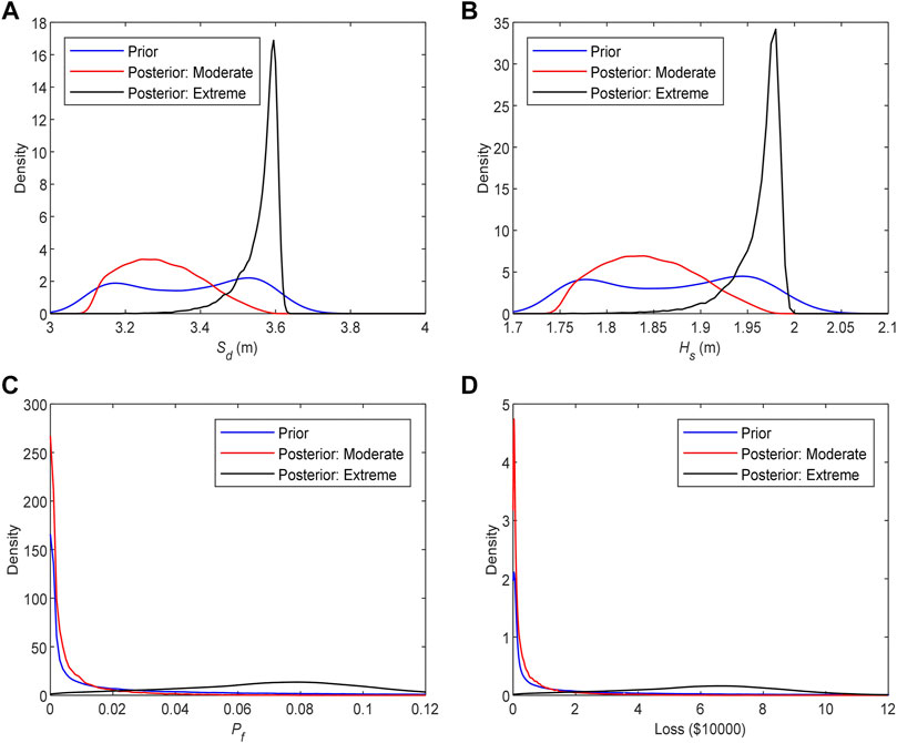
FIGURE 8. The effect of different sets of evidence (moderate vs. extreme climate scenario) in the marginal posterior distribution of the loss for the year 2050.

Finally, to illustrate how new evidence updates the posterior distribution of all the random variables that are inside the Markov blanket, Figure 9 shows the change in the posterior distribution of RCP under the two different climate scenarios. It is apparent that the parent node ($U$) also gets updated once information is obtained for the children nodes ($V_f$ and $SLR)$. This means that we can know more about the distribution of any RV in the Markov Blanket even with one set of evidence, which acts as an added advantage of using BN to model engineering problems, where the information is usually limited to certain parameters of the model.

FIGURE 9

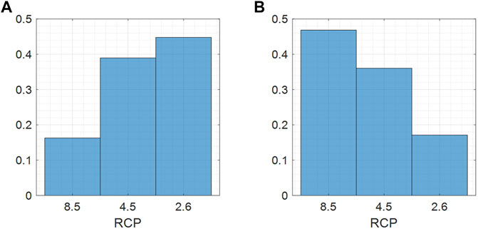
FIGURE 9. Variation in the posterior distribution of RCP under the two different climate scenarios: (A) moderate, and (B) extreme.

Representative System: Two Single-Bay Elastoplastic Bay

In this example, the impact of cascading effects and time-varying parameters in the marginal distribution of the DV are investigated. A system consisting of two single-bay elastoplastic frames is used to illustrate the effects of cascading failure in the form of debris load (Figures 10A,B). Moreover, the time-varying parameters of the system are incorporated into the analysis using a DBN representation of the PBCE framework. The single-bay frame structure is adapted from (Der Kiureghian, 2005; Straub and Der Kiureghian, 2010). Due to computational constraints, a service life of 15 years instead of the 20-years from the original example (Straub and Der Kiureghian, 2010), is selected for both the frames to illustrate the DBN modeling of the PBCE framework. Both frames are subjected to the same vertical $V$ (dead) and time-varying horizontal $H\left(t\right)$ (environmental) loads $\left(\mathbf{\Theta }=V,H\left(t\right) \right)$. Herein, the time-varying horizontal $H\left(t\right)$ load represents the annual maximum load in the year of analysis. To account for possible common influencing factors (e.g. hazard model, statistical uncertainties) (Straub and Der Kiureghian, 2010) in $H\left(t\right)$, the probability distribution of $H\left(t\right)$ is conditioned on a random influencing variable $U_H$.

FIGURE 10

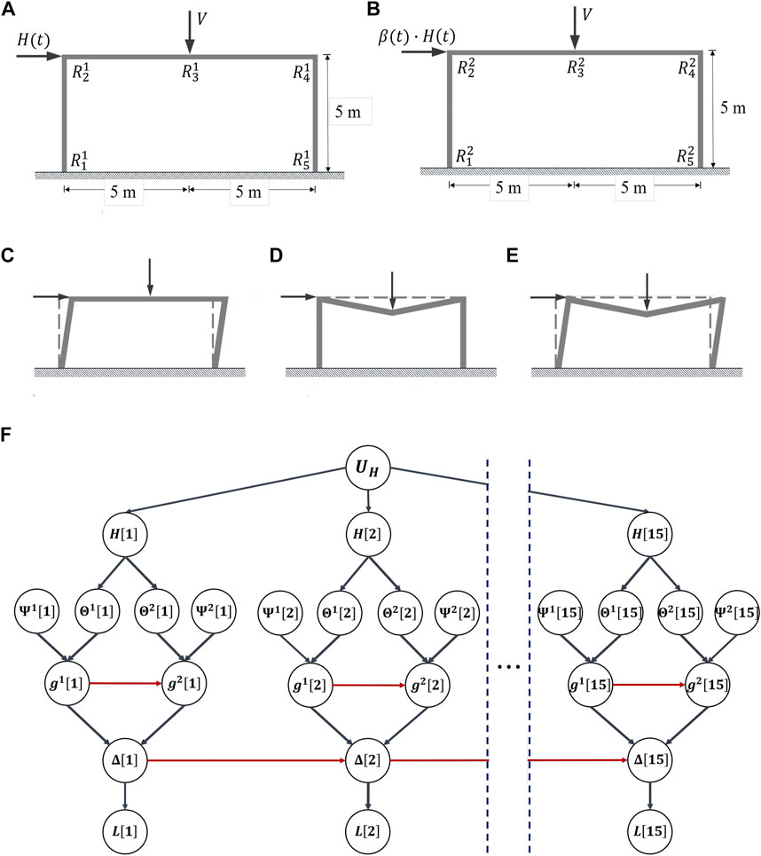
FIGURE 10. Typical single-bay elastoplastic frame model adapted from (Der Kiureghian, 2005; Straub and Der Kiureghian, 2010). In the two-frame system, each frame is subjected to vertical $V$ and time-varying horizontal $H\left(t\right)$ loads. (A) Frame 1, (B) Frame 2 is subjected to an additional horizontal load as a result of the structural failure of Frame 1. Three different structural failure mechanisms are considered: (C) sway mechanism, (D) beam mechanism, and (E) combined mechanism. (F) DBN model for the system of two single-bay elastoplastic frames.

Three different structural failure mechanisms (i.e. sway (Figure 10C), beam (Figure 10D), and combined (Figure 10E)) are defined for each frame by the limit-state functions presented in Eq. 24a, Eq. 24b, and Eq. 24c, where the capacity is given by the five plastic-moment capacities for both of the frames $\left({\mathbf{\Psi }}^i=R_1^i,R_2^i,R_3^i,R_4^i,R_5^i \right)$, with $i=\mathrm{1,2}$.

$g_1^i\left({\mathbf{x}}^{\mathbf{i}}\right)=r_1^i+r_2^i+r_4^i+r_5^i-5h(\mathrm{24a})$

$g_2^i\left({\mathbf{x}}^{\mathbf{i}}\right)=r_2^i+2r_3^i+r_4^i-5v(\mathrm{24b})$

$g_3^i\left({\mathbf{x}}^{\mathbf{i}}\right)=r_1^i+2r_3^i+2r_4^i+r_5^i-5h-5v(\mathrm{24c})$

where $r_1^i,r_2^i,\cdots ,r_5^i$ are the random realization of the plastic-moment capacities of the $i^{th}$ frame, $v$ is the random realization of the vertical load for the $i^{th}$ frame, $h$ is the realization of the horizontal load for the $i^{th}$ frame, ${\mathbf{x}}^{\mathbf{i}}=\left\{r_1^i,r_2^i,r_3^i,r_4^i,r_5^i,v,h\right\}$ is the vector of random variables defining the limit-state functions, and $g_1^i\left(\mathbf{x}\right)$, $g_2^i\left(\mathbf{x}\right)$ , $g_3^i\left(\mathbf{x}\right)$ are the limit-state functions defining the sway, beam, and combined failure mechanism for the $i^{th}$ frame, respectively. To incorporate the possibility of cascading failure, it is assumed that in the event of failure of the first frame, the debris generated will act as an additional lognormally distributed horizontal load [$AL\left(t\right)$] in the second frame. Therefore, $H\left(t\right)=\beta \left(t\right)\cdot H\left(t\right)$, where $\beta \left(t\right)=\left(1+AL\left(t\right)/H\left(t\right)\right)$, and the limit state functions are modified accordingly. Herein, the variables presented in capital letters correspond to random variables, whose probabilistic description is given in Table 3. Figure 10F presents the DNB representation of the system.

TABLE 3

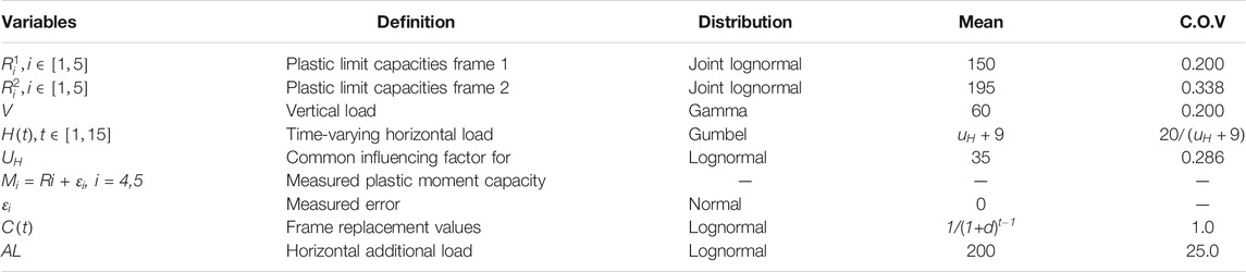
TABLE 3. A probabilistic model for the two single-bay elastoplastic frames system. Forces are in units of $kN$ and moments in units of $kN-m$.

Two decision variables associated with the expected economic loss in case of failure of the system are investigated in this case study, the 1) service-life loss $L_s$, with no repair or replacement action during the 15-years service life of the structure, and the 2) aggregated loss $L_A$, considering that in the event of failure, the system is replaced by the end of the year. Eq. 25a, Eq. 25b, Eq. 25c, Eq. 26a, Eq. 26b, Eq. 26c, and Eq. 26d present the mathematical description of the service-life and the aggregated loss, respectively. Using Eq. 25a, Eq. 25b, and Eq. 25c, the service-life loss at the end of 15 years, $L_S\left[15\right]$, is obtained by performing recursive computation from $t=1$ to $t=15$. The service-life loss considers the loss in present value encountered at the end of the 15-years service-life given that failure has occurred in any of the 15 years. Therefore, at each year $\left[t\right]$ information about the state of the system (failed or not failed) in the previous year $\left[t-1\right]$ is needed to evaluate the current state of the system. Consequently, if the system has failed in the year $\left[t\right]$, it will remain in this state for the following years, as represented by the link connecting the damage variable $\mathbf{\Delta }$ through the lifetime of the system in Figure 10F. On the other hand, the aggregated loss represents the cumulative loss (assuming replacement after each damage scenario) in the present value, at the end of the service life of the system. The aggregated loss will therefore represent the cumulative loss of all the replacements that the system underwent during its 15-years lifetime. In this case, no flow of information is needed on a year-to-year basis, because no previous information in the state of the system is required (the system would be considered in as-new condition at the beginning of every year). In both instances, the losses are computed based on the replacement value of the frames, $C\left(t\right)$, where the inflation-adjusted discount rate $d$ is set to 3% (Table 3).

OpenBUGS (Spiegelhalter et al., 2007) is used to implement the DBN model of the two scenarios previously discussed for the cascading and no-cascading cases. The convergence of the MCMC simulation is ensured by computing the Gelman-Rubin statistic $\widehat{R}$ (Gelman and Rubin, 1992) corresponding to various starting iteration steps (Figure 4B). Two chains of Markov chain Monte Carlo are generated to draw 20,000 samples from the target stationary distribution, with 5,000 samples discarded during the tunning process.

$L_S\left[t\right]=C_1\left[t\right]\cdot {\text{Δ}}_{1\_S}\left[t\right]+C_2\left[t\right]\cdot {\text{Δ}}_{2\_S}\left[t\right](\mathrm{25a})$

${\text{Δ}}_{1\_S}\left[t\right]=max\left(\frac{1+sign\left(g_1\left[t\right]\right)}{2},{\text{Δ}}_{1\_S}\left[t-1\right]\right)(\mathrm{25b})$

${\text{Δ}}_{2\_S}\left[t\right]=max\left(\frac{1+sign\left(g_2\left[t\right]\right)}{2},{\text{Δ}}_{2\_S}\left[t-1\right]\right)(\mathrm{25c})$

$L_A={\displaystyle \sum _{t=1}^{15}L\left[t\right]}(\mathrm{26a})$

$L\left[t\right]=C\left[t\right]\cdot \left({\text{Δ}}_{1\_A}\left[t\right]+{\text{Δ}}_{2\_A}\left[t\right]\right)(\mathrm{26b})$

${\text{Δ}}_{1\_A}\left[t\right]=\frac{1+sign\left(g_1\left[t\right]\right)}{2}(\mathrm{26c})$

${\text{Δ}}_{2\_A}\left[t\right]=\frac{1+sign\left(g_2\left[t\right]\right)}{2}(\mathrm{26d})$

Results and Discussion

Effect of Cascading Failure

The effect of cascading failure is analyzed by comparing the exceedance probability and density function of the normalized service-life loss $L_s$ with and without the consideration of cascading failure. Figure 11A depicts the probability of exceeding a particular value of normalized loss for both cases at the end of 15 years. From the analysis, it is apparent that the incurred loss for any level of exceedance probability is underestimated if the effect of cascading failure is neglected. For instance, for a probability of exceedance of 1.0% the rise in the service-life loss is as high as 70%. For a 10% exceedance probability, the percentage rise in loss is even more significant, with a change of 87% in $L_s$ when considering cascading effects. Moreover, Figure 11B illustrates that the uncertainty of the conditional distribution of the normalized service-life loss given that at least one of the two frames has been damaged is also underestimated in the non-cascading case. Figure 12A shows the variation of the normalized service-life loss during the 15-years service life of the structure corresponding to 1 and 5% exceedance probability of loss, with and without the consideration of the effect of cascading failure. In both cases, incorporating the cascading effect in the loss analysis remains significant throughout the system’s service life. Nevertheless, for a 5% exceedance probability, the incurred loss is zero for both the cascading and no-cascading case up to the third year of life of the system. This means that there is a 95% probability that the system will not experience any loss until the fourth year.

FIGURE 11

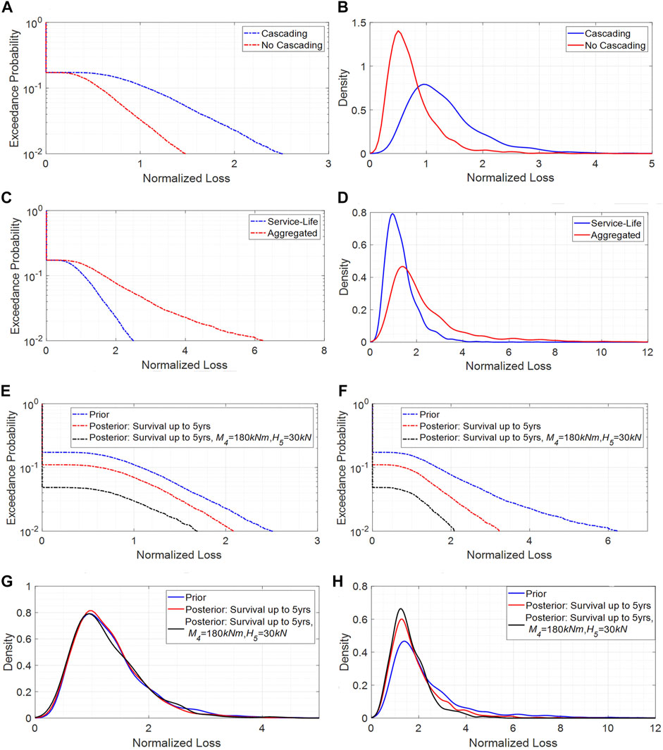
FIGURE 11. (A) Variation of exceedance probability corresponding to its normalized loss with and without the consideration of the effect of cascading failure, (B) conditional distribution of the normalized loss given at least one of the two frames have damaged, for both sets of analysis with and without considering cascading effect. (C) Comparison of the exceedance probability of normalized service-life loss and aggregated loss at the end of 15 years, (D) conditional distribution of the normalized service-life loss and aggregated loss given that at least one of the two frames have damage at the end of 15 years. The prior and posterior variation of exceedance probability corresponding to its (E) normalized service-life loss and (F) normalized aggregated loss at the end of 15 years. The conditional prior and posterior distributions of the (G) normalized service-life loss and (H) normalized aggregated loss given that at least one of the two frames have damage at the end of 15 years.

FIGURE 12

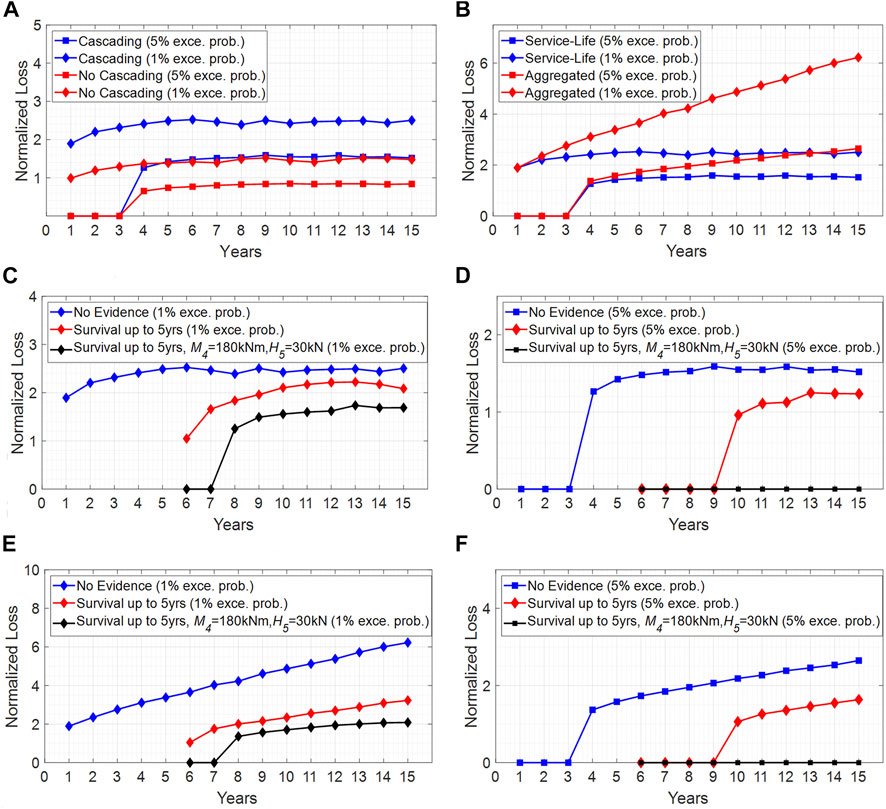
FIGURE 12. (A) Normalized loss corresponding to 1 and 5% exceedance probability for varying service-life, with and without the consideration of the effect of cascading failure, (B) normalized service-life loss and aggregated loss corresponding to 1 and 5% exceedance probability for varying service-life, (C) the prior and posterior normalized service-life loss corresponding to (C) 1% and (D) 5% exceedance probability for varying service-life, (E) the prior and posterior normalized aggregate loss corresponding to (E) 1% and (F) 5% exceedance probability for varying service-life 1 and 15 years.

Service-Life Loss Compared to Aggregated Loss

Having established the importance of considering cascading effects, the results from the present and following sections consider cascading failure in the analysis. Figure 11C presents a comparison of the exceedance probability for the normalized service-life loss and aggregated loss at the end of 15 years. As expected, the exceedance probability of aggregated loss is more than service-life loss due to recurrent repair of the system after each damage. Moreover, the assumption of repair after each damage scenario increases the uncertainty of aggregated loss compared to the service-life loss as observed in the conditional distribution of the normalized service-life loss and aggregated loss given that at least one of the two frames have damage at the end of 15 years, as shown in Figure 11D. The normalized service-life loss and aggregated loss corresponding to 1 and 5% exceedance probability for varying service-life between 1 and 15 years are depicted in Figure 12B. The assumption of repair after each damage scenario naturally increases the corresponding aggregated loss compared to the case of service-life loss over time. Moreover, when comparing the change of service-life and aggregated loss during the 15-years of analysis, it is seen that the difference between the 5 and 1% probability of exceedance of the service-life loss is significantly lower compared to the aggregated loss. This shows that the probability density function of the aggregated loss has a longer upper tail than the service-life loss distribution and that this difference increases in time, as seen by the growing gap between the 1 and 5% probability of exceedance (red curves in Figure 12B).

Effect of Evidence in Service-Life Loss and Aggregated Loss

As discussed in Dynamic Bayesian Network Modeling of the Performance-Based Coastal Engineering Framework, the proposed dynamic Bayesian network model enables updating of the prior distribution of the network variables to obtain the posterior distributions when evidence about any variable emerges, both qualitative and quantitative. In this section, two sets of evidence are considered which are observed at the end of 5 years for exemplification purposes. The first one involves qualitative evidence about both of the frames where it is observed that both frames have survived until then (i.e. no observed damage to the frame at the end of 5 years). The second set includes both qualitative and quantitative evidence. In addition to the observation of the 5-years survival of both frames, quantitative evidence about the structure and the hazard are observed at the end of the fifth year. Specifically, the plastic moment capacity at $R_4^i$ in Figures 10A,B ($M_4$) and the horizontal load $H\left(t\right)$ are measured respectively to be 180 and 30 kN with their associated measurement noise as specified in Table 3. Figures 11E,F presents the prior and posterior exceedance probability corresponding to the normalized service-life (Figure 11E) and aggregated loss (Figure 11F) at the end of 15 years. In both cases, the posterior probability of exceedance of loss is sensitive to observed evidence. The conditional prior and posterior distributions of the normalized service-life loss given that at least one of the two frames have damage at the end of 15 years are presented in Figure 11G. The posterior distribution of loss conditioned on the occurrence of damage to at least one frame in their service life for the observed evidence does not change compared to the conditional prior distribution. It is assumed that in the case of service-life loss analysis, the system will not be repaired till 15 years. As the occurrence of loss is not aggregated together over the years, the probability of loss for a particular year only depends on the probability of damage of the system leading up to that year. Hence, the prior or the posterior distribution of the service-life loss conditioned on the occurrence of damage to the system shows no significant variation. Similarly, the uncertainty of conditional posterior aggregated loss reduces with observed evidence due to the assumption of repair after each damage scenario in the case of aggregated loss as observed in Figure 11H.

Figures 12C–D present the prior and posterior normalized service-life loss corresponding to 1% (Figure 12C) and 5% (Figure 12D) exceedance probability between 1 and 15 years. In both cases, the posterior marginal distribution of the loss is sensitive to observed evidence. Moreover, the incorporation of both qualitative and quantitative evidence significantly reduces the probability of incurred service-life loss, when compared to the prior and qualitative-only marginal distributions of the loss. Figure 12D shows that there is a 95% probability that the incurred service-life loss is zero when the two sets of evidence are observed. This behavior is also observed in the marginal distribution of the aggregated loss, as per Figures 12E,F.

Conclusion

The proposed performance-based coastal engineering framework provides a methodology for system performance assessment focused on coastal systems that incorporates new concepts such as time-varying and event-triggered factors into the analysis. The framework consists of six basic components: performance objectives, hazard analysis, structural characterization, structural analysis, damage analysis, and performance analysis. The framework is flexible enough to accommodate multi-hazard scenarios, systems with multiple structures, cascading-effects, and different performance metrics. To compute the marginal probability distribution of the decision variable, this study proposes the implementation of a probabilistic graphical model in the form of a dynamic Bayesian network. DBNs allow modeling the causal dependence among the variables, offering an efficient sampling strategy and facilitating communication with stakeholders and easy incorporation of expert knowledge. The dynamic Bayesian network is constructed based on the relevant parameters of the system, only needing their probabilistic description or estimates. In cases with no information of the probabilistic description of the parameters, non-informative priors can be used, such as a uniform distribution having limits based on engineering judgment or “best estimates”. Moreover, DBNs allow the incorporation of evidence, increasing the confidence of the parameter estimates through Bayesian updating. Two case studies showcase the application of the framework. The first one explored the effects of time-varying factors in the performance assessment of a typical elevated residential structure subjected to surge and wave loads for the years 2030, 2050, and 2100. Results showed the sensitivity of the probability of failure and probable loss of the house to the climate conditions, especially to the $SLR$, which increments the probability of high water-levels at the site of the structure. It was found that given the conditions assumed in this study, the house might be deemed as structurally safe up to the year 2050, after which the probability of failure is heavily skewed toward the complete failure scenario in the year 2100. As evidence was observed, the posterior marginal distribution of the loss presented a reduced variance when compared to the prior distribution, given the margin of error of the measurements assumed in the study. The second case study explored the effect of cascading failure in both the service-life and aggregated loss of a system of two single-bay frames. The constructed DBN of the system illustrated the year-to-year updating of the model and the incorporation of both qualitative and quantitative evidence in the analysis of the network. The results showed that neglecting cascading effects significantly underestimates the probability of exceedance of the loss and its associated uncertainty.

Future studies will incorporate a fully probabilistic time-varying hazard model to probabilistically characterize the intensity parameters acting upon the structure for each year and its respective annual probability of exceedance. Moreover, real systems consisting of multiple structures or sub-components can be used as test beds of the framework to quantify the impact of cascading effects in a full probabilistic manner, as well as incorporating multi-hazard settings. Future directions of study can also include the consideration of feedback loops such as the change of performance objectives due to non-acceptable values of the decision variables or new inputs during the decision analysis component. Likewise, the framework can also be used to evaluate systems considering more than one decision variable and investigate optimization techniques to make decisions based on the analysis. Related opportunities in the field include the advancement of fragility functions specific to coastal structures and $n$-dimensional hazard surfaces characterizing the rates of joint intensity parameters exceedance. The PBCE framework should also be applied to inform adaptation engineering strategies for evaluating different retrofitting measures that consider the effects of a changing climate. The sensitivity of the results to different sets of evidence and different ranges of measurement error should also be addressed. However, data related to relevant parameters of coastal systems is often scarce, such as site-specific sea-level rise estimates or structure-wise structural data (e.g., elevation of the house with respect to the ground), and even non-existing in some parts of the world. Therefore, efforts should also be directed toward the creation of a comprehensive dataset specific to coastal systems, including but not limited to repair costs of structural elements, change in property value in coastal areas, costs of retrofitting strategies, downtimes, frequency of maintenance, insurance claims regarding coastal hazards, among others, to better inform the probabilistic models. Ongoing work is considering the extension of the proposed PBCE framework to support resilience strategies by identifying vulnerable areas in coastal communities under climate change conditions.

Data Availability Statement

The raw data supporting the conclusion of this article will be made available by the authors, without undue reservation.

Author Contributions

CG-D: conceptualization, methodology, data collection, modeling, analysis, investigation, visualization, writing—original draft. JP: conceptualization, supervision, writing—review and editing, funding acquisition, project administration.

Conflict of Interest

The authors declare that the research was conducted in the absence of any commercial or financial relationships that could be construed as a potential conflict of interest.

Acknowledgments

The authors gratefully acknowledge the financial support of this research by the National Science Foundation under awards No. OISE-1545837 and CMMI-2002522.

References

American Society of Civil Engineers (2017). Seismic Evaluation and Retrofit of Existing Buildings.

Ataei, N., and Padgett, J. E. (2013). Limit State Capacities for Global Performance Assessment of Bridges Exposed to hurricane Surge and Wave. Struct. Saf. 41, 73–81. doi:10.1016/j.strusafe.2012.10.005

CrossRef Full Text | Google Scholar

Attary, N., Unnikrishnan, V. U., van de Lindt, J. W., Cox, D. T., and Barbosa, A. R. (2017). Performance-Based Tsunami Engineering Methodology for Risk Assessment of Structures. Eng. Structures 141, 676–686. doi:10.1016/j.engstruct.2017.03.071

CrossRef Full Text | Google Scholar

Attary, N., Van De Lindt, J. W., Barbosa, A. R., Cox, D. T., and Unnikrishnan, V. U. (2019). Performance-Based Tsunami Engineering for Risk Assessment of Structures Subjected to Multi-Hazards: Tsunami Following Earthquake. J. Earthquake Eng. 2019, 1–20. doi:10.1080/13632469.2019.1616335

CrossRef Full Text | Google Scholar

Baade, R. A., Baumann, R., and Matheson, V. (2007). Estimating the Economic Impact of Natural and Social Disasters, with an Application to Hurricane Katrina. Urban Stud. 44 (11), 2061–2076. doi:10.1080/00420980701518917

CrossRef Full Text | Google Scholar

Balomenos, G. P., and Padgett, J. E. (2018). Fragility Analysis of Pile-Supported Wharves and Piers Exposed to Storm Surge and Waves. J. Waterway, Port, Coastal Ocean Eng. 144 (2), 04017046. doi:10.1061/(ASCE)WW.1943-5460.0000436

CrossRef Full Text | Google Scholar

Baradaranshoraka, M., Pinelli, J.-P., Gurley, K., Zhao, M., Peng, X., and Paleo-Torres, A. (2019). Characterization of Coastal Flood Damage States for Residential Buildings. Asce-asme J. Risk Uncertainty Eng. Syst. Part. A: Civ. Eng. 5 (1), 04019001. doi:10.1061/AJRUA6.0001006

CrossRef Full Text | Google Scholar

Barbato, M., Petrini, F., Unnikrishnan, V. U., and Ciampoli, M. (2013). Performance-Based Hurricane Engineering (PBHE) Framework. Struct. Saf. 45, 24–35. doi:10.1016/j.strusafe.2013.07.002

CrossRef Full Text | Google Scholar

Becker, A. H., Matson, P., Fischer, M., and Mastrandrea, M. D. (2015). Towards Seaport Resilience for Climate Change Adaptation: Stakeholder Perceptions of hurricane Impacts in Gulfport (MS) and Providence (RI). Prog. Plann. 99, 1–49. doi:10.1016/j.progress.2013.11.002

CrossRef Full Text | Google Scholar

Bensi, M., Kiureghian, A. D., and Straub, D. (2013). Efficient Bayesian Network Modeling of Systems. Reliability Eng. Syst. Saf. 112, 200–213. doi:10.1016/j.ress.2012.11.017

CrossRef Full Text | Google Scholar

Berlemann, M. (2016). Does hurricane Risk Affect Individual Well-Being? Empirical Evidence on the Indirect Effects of Natural Disasters. Ecol. Econ. 124, 99–113. doi:10.1016/j.ecolecon.2016.01.020

CrossRef Full Text | Google Scholar

Bernier, C., and Padgett, J. E. (2019). Fragility and Risk Assessment of Aboveground Storage Tanks Subjected to Concurrent Surge, Wave, and Wind Loads. Reliability Eng. Syst. Saf. 191, 106571. doi:10.1016/j.ress.2019.106571

CrossRef Full Text | Google Scholar

Bjarnadottir, S., Li, Y., Reynisson, O., and Stewart, M. G. (2018). Reliability-based Assessment of Climatic Adaptation for the Increased Resiliency of Power Distribution Systems Subjected to Hurricanes. Sustainable Resilient Infrastructure 3 (1), 36–48. doi:10.1080/23789689.2017.1345255

CrossRef Full Text | Google Scholar

Bjarnadottir, S., Li, Y., and Stewart, M. G. (2011). A Probabilistic-Based Framework for Impact and Adaptation Assessment of Climate Change on hurricane Damage Risks and Costs. Struct. Saf. 33 (3), 173–185. doi:10.1016/j.strusafe.2011.02.003

CrossRef Full Text | Google Scholar

Blake, E. S., Kimberlain, T. B., Berg, R. J., CangiaLosi, J. P., and Beven, J. L. (2013). Tropical Cyclone Report Hurricane Sandy (AL182012) 22–29. doi:10.1017/CBO9781107415324.004

CrossRef Full Text

Blake, E. S., and Zelinsky, D. A. (2018). National Hurricane Center Tropical Cyclone Report. Hurricane Harvey.

Briaud, J. L. (2015). Scour Depth at Bridges: Method Including Soil Properties. I: Maximum Scour Depth Prediction. J. Geotechnical Geoenvironmental Eng. 141 (2), 1–13. doi:10.1061/(ASCE)GT.1943-5606.0001222

CrossRef Full Text | Google Scholar

Camargo, S. J., and Wing, A. A. (2021). Increased Tropical Cyclone Risk to Coasts. Science 371 (6528), 458–459. doi:10.1126/science.abg3651

PubMed Abstract | CrossRef Full Text | Google Scholar

Carther, S. (2020). Understanding the Time Value of Money. Investopedia. https://www.investopedia.com/articles/03/082703.asp.

Cavalli, A., Cibecchini, D., Togni, M., and Sousa, H. S. (2016). A Review on the Mechanical Properties of Aged wood and Salvaged Timber. Construction Building Mater. 114, 681–687. doi:10.1016/j.conbuildmat.2016.04.001

CrossRef Full Text | Google Scholar

Chen, J. (2020). Future Value (FV). Investopedia. https://www.investopedia.com/terms/f/futurevalue.asp.

Choe, D.-E., Gardoni, P., Rosowsky, D., and Haukaas, T. (2008). Probabilistic Capacity Models and Seismic Fragility Estimates for RC Columns Subject to Corrosion. Reliability Eng. Syst. Saf. 93 (3), 383–393. doi:10.1016/j.ress.2006.12.015

CrossRef Full Text | Google Scholar

Ciampoli, M., Petrini, F., and Augusti, G. (2011). Performance-Based Wind Engineering: Towards a General Procedure. Struct. Saf. 33 (6), 367–378. doi:10.1016/j.strusafe.2011.07.001

CrossRef Full Text | Google Scholar

Crews, K. I., and MacKenzie, C. (2008). Development of Grading Rules for Re-cycled Timber Used in Structural Applications. World Conference on Timber Engineering. hdl.handle.net/10453/11172.

Cui, W., and Caracoglia, L. (2018). A Unified Framework for Performance-Based Wind Engineering of Tall Buildings in hurricane-prone Regions Based on Lifetime Intervention-Cost Estimation. Struct. Saf. 73, 75–86. doi:10.1016/j.strusafe.2018.02.003

CrossRef Full Text | Google Scholar

Daniell, J. E., Schaefer, A. M., Wenzel, F., and Kunz-Plapp, T. (2015). The Value of Life in Earthquakes and Other Natural Disasters: Historical Costs and the Benefits of Investing in Life Safety. Proc. Tenth Pac. Conf. Earthquake Eng. 130.

Google Scholar

de Boer, J., Botzen, W. J. W., and Terpstra, T. (2016). Flood Risk and Climate Change in the Rotterdam Area, The Netherlands: Enhancing Citizen's Climate Risk Perceptions and Prevention Responses Despite Skepticism. Reg. Environ. Change 16 (6), 1613–1622. doi:10.1007/s10113-015-0900-4

CrossRef Full Text | Google Scholar

Dehghani, N. L., and Shafieezadeh, A. (2019). “Probabilistic Sustainability Assessment of Bridges Subjected to Multi-Occurrence Hazards,” in International Conference on Sustainable Infrastructure 2019: Leading Resilient Communities through the 21st Century, 555–565. doi:10.1061/9780784482650.059

CrossRef Full Text | Google Scholar

Der Kiureghian, A. (2005). “First- and Second-Order Reliability Methods,” in Engineering Design Reliability Handbook, 1–24.

Google Scholar

Ditlevsen, O., and Friis-Hansen, P. (2009). Cost and Benefit Including Value of Life, Health and Environmental Damage Measured in Time Units. Struct. Saf. 31 (2), 136–142. doi:10.1016/j.strusafe.2008.06.010

CrossRef Full Text | Google Scholar

Do, T. Q., van de Lindt, J. W., and Cox, D. T. (2020). Hurricane Surge-Wave Building Fragility Methodology for Use in Damage, Loss, and Resilience Analysis. J. Struct. Eng. 146 (1), 04019177. doi:10.1061/(asce)st.1943-541x.0002472

CrossRef Full Text | Google Scholar

Do, T. Q. (2016). Fragility Approach for Performance-Based Design in Fluid-Structure Interaction Problems, Part I: Wind and Wind Turbines, Part II: Waves and Elevated Coastal Structures. Colorado State University.

Do, T. Q., van de Lindt, J. W., and Cox, D. T. (2016). Performance-based Design Methodology for Inundated Elevated Coastal Structures Subjected to Wave Load. Eng. Structures 117, 250–262. doi:10.1016/j.engstruct.2016.02.046

CrossRef Full Text | Google Scholar

Dong, Y., and Li, Y. (2016). Risk-based Assessment of wood Residential Construction Subjected to hurricane Events Considering Indirect and Environmental Loss. Sust. Resilient Infrastructure 1 (1–2), 46–62. doi:10.1080/23789689.2016.1179051

CrossRef Full Text | Google Scholar

Ebad Sichani, M., Anarde, K. A., Capshaw, K. M., Padgett, J. E., Meidl, R. A., Hassanzadeh, P., et al. (2020). Hurricane Risk Assessment of Petroleum Infrastructure in a Changing Climate. Front. Built Environ. 6, 104. doi:10.3389/fbuil.2020.00104

CrossRef Full Text | Google Scholar

Ebersole, B. A., Massey, T. C., Melby, J. A., Nadal-Caraballo, N. C., Hendon, D. L., Richardson, T. W., et al. (2017). Interim Report—IKE dike Concept for Reducing hurricane Storm Surge in the Houston-Galveston Region. Jackson: MS.

Ellingwood, B. R., and Lee, J. Y. (2016). Life Cycle Performance Goals for Civil Infrastructure: Intergenerational Risk-Informed Decisions. Struct. Infrastructure Eng. 12 (7), 822–829. doi:10.1080/15732479.2015.1064966

CrossRef Full Text | Google Scholar

Emanuel, K. (2017). Assessing the Present and Future Probability of Hurricane Harvey's Rainfall. Proc. Natl. Acad. Sci. USA 114 (48), 12681–12684. doi:10.1073/pnas.1716222114

PubMed Abstract | CrossRef Full Text | Google Scholar

Federal Emergency Management Agency (FEMA) and U.S. Army Corps of Engineers (USACE) (2011). Flood Insurance Study: Coastal Counties. Texas.

Federal Emergency Management Agency (FEMA) (2011). FEMA P-55 Coastal Conctruction Manual.

FEMA (2013). Flood Insurance Study - Harris County. Texas and Incorporated Areas.

FEMA (2009). Hurricane Ike in Texas and Louisiana: Mitigation Assessment Team Report, Building Performance Observations, Recommendations, and Technical Guidance. FEMA P-757. https://www.fema.gov/media-library-data/20130726-1648-20490-9826/fema757.pdf.

Fereshtehnejad, E., Gidaris, I., Rosenheim, N., Tomiczek, T., Padgett, J. E., Cox, D. T., et al. (2021). Probabilistic Risk Assessment of Coupled Natural-Physical-Social Systems: Cascading Impact of Hurricane-Induced Damages to Civil Infrastructure in Galveston, Texas. Nat. Hazards Rev. 22 (3), 04021013. doi:10.1061/(ASCE)NH.1527-6996.0000459

CrossRef Full Text | Google Scholar

Field, C. B., Barros, V., Stocker, T. F., and Dahe, Q. (2012). Managing the Risks of Extreme Events and Disasters to advance Climate Change Adaptation. Cambridge University Press.

Gardoni, P., Der Kiureghian, A., and Mosalam, K. M. (2002). Probabilistic Capacity Models and Fragility Estimates for Reinforced concrete Columns Based on Experimental Observations. J. Eng. Mech. 128 (10), 1024–1038. doi:10.1061/(asce)0733-9399(2002)128:10(1024)

CrossRef Full Text | Google Scholar

Gelman, A., and Rubin, D. B. (1992). Inference from Iterative Simulation Using Multiple Sequences. Statist. Sci. 7 (4), 457–472. doi:10.1214/ss/1177011136

CrossRef Full Text | Google Scholar

Ghahramani, Z. (1998). Learning Dynamic Bayesian Networks. International School on Neural Networks, Initiated by IIASS and EMFCSC, 168–197. doi:10.1007/BFb0053999

CrossRef Full Text

Gonzalez Duenas, C., Bernier, C., and Padgett, J. (2019). Probabilistic Assessment of Bridges Subjected to Waterborne Debris. Coastal Structures 2019, 356–365. doi:10.18451/978-3-939230-64-9_036

CrossRef Full Text | Google Scholar

Gordian (2019). Square Foot Costs with RSMeans Data.

Günay, S., and Mosalam, K. M. (2013). PEER Performance-Based Earthquake Engineering Methodology, Revisited. J. Earthquake Eng. 17 (6), 829–858. doi:10.1080/13632469.2013.787377

CrossRef Full Text | Google Scholar

Hallowell, S. T., Myers, A. T., Arwade, S. R., Pang, W., Rawal, P., Hines, E. M., et al. (2018). Hurricane Risk Assessment of Offshore Wind Turbines. Renew. Energ. 125, 234–249. doi:10.1016/j.renene.2018.02.090

CrossRef Full Text | Google Scholar

Hassanzadeh, P., Lee, C.-Y., Nabizadeh, E., Camargo, S. J., Ma, D., and Yeung, L. Y. (2020). Effects of Climate Change on the Movement of Future Landfalling Texas Tropical Cyclones. Nat. Commun. 11 (1), 1–9. doi:10.1038/s41467-020-17130-7

PubMed Abstract | CrossRef Full Text | Google Scholar

Hatzikyriakou, A., Lin, N., Gong, J., Xian, S., Hu, X., and Kennedy, A. (2016). Component-based Vulnerability Analysis for Residential Structures Subjected to Storm Surge Impact from Hurricane Sandy. Nat. Hazards Rev. 17 (1), 05015005. doi:10.1061/(ASCE)NH.1527-6996.0000205

CrossRef Full Text | Google Scholar

Hu, X., Liu, B., Wu, Z. Y., and Gong, J. (2016). Analysis of Dominant Factors Associated with Hurricane Damages to Residential Structures Using the Rough Set Theory. Nat. Hazards Rev. 17 (3), 1–10. doi:10.1061/(ASCE)NH.1527-6996.0000218

CrossRef Full Text | Google Scholar

Jia, G., and Taflanidis, A. A. (2013). Kriging Metamodeling for Approximation of High-Dimensional Wave and Surge Responses in Real-Time Storm/hurricane Risk Assessment. Comp. Methods Appl. Mech. Eng. 261-262, 24–38. doi:10.1016/j.cma.2013.03.012

CrossRef Full Text | Google Scholar

Jonkman, S. N. (2007). Loss of Life Estimation in Flood Risk Assessment; Theory and Applications. doi:10.1142/9789812709554_0118

CrossRef Full Text

Ju, C., Ning, Y., and Pan, W. (2016). A Review of Interdependence of Sustainable Building. Environ. Impact Assess. Rev. 56, 120–127. doi:10.1016/j.eiar.2015.09.006

CrossRef Full Text | Google Scholar

Kameshwar, S., Cox, D. T., Barbosa, A. R., Farokhnia, K., Park, H., Alam, M. S., et al. (2019). Probabilistic Decision-Support Framework for Community Resilience: Incorporating Multi-Hazards, Infrastructure Interdependencies, and Resilience Goals in a Bayesian Network. Reliability Eng. Syst. Saf. 191, 106568. doi:10.1016/j.ress.2019.106568

CrossRef Full Text | Google Scholar

Kameshwar, S., and Padgett, J. E. (2018). Parameterized Fragility Assessment of Bridges Subjected to Pier Scour and Vehicular Loads. J. Bridge Eng. 23 (7), 1–11. doi:10.1061/(ASCE)BE.1943-5592.0001240

CrossRef Full Text | Google Scholar

Khakzad, N., and Van Gelder, P. (2018). Vulnerability of Industrial Plants to Flood-Induced Natechs: A Bayesian Network Approach. Reliability Eng. Syst. Saf. 169, 403–411. doi:10.1016/j.ress.2017.09.016

CrossRef Full Text | Google Scholar

Kopp, R. E., Horton, R. M., Little, C. M., Mitrovica, J. X., Oppenheimer, M., Rasmussen, D. J., et al. (2014). Probabilistic 21st and 22nd century Sea‐level Projections at a Global Network of Tide‐gauge Sites. Earth's Future 2 (8), 383–406. doi:10.1002/2014ef000239

CrossRef Full Text | Google Scholar

Kousky, C. (2014). Informing Climate Adaptation: A Review of the Economic Costs of Natural Disasters. Energ. Econ. 46, 576–592. doi:10.1016/j.eneco.2013.09.029

CrossRef Full Text | Google Scholar

Landefeld, J. S., and Seskin, E. P. (1982). The Economic Value of Life: Linking Theory to Practice. Am. J. Public Health 72 (6), 555–566. doi:10.2105/AJPH.72.6.555

PubMed Abstract | CrossRef Full Text | Google Scholar

Lee, J. Y., and Ellingwood, B. R. (2017). A Decision Model for Intergenerational Life-Cycle Risk Assessment of Civil Infrastructure Exposed to Hurricanes under Climate Change. Reliability Eng. Syst. Saf. 159 (10), 100–107. doi:10.1016/j.ress.2016.10.022

CrossRef Full Text | Google Scholar

Lerner, U., Segal, E., and Koller, D. (2013). Exact Inference in Networks with Discrete Children of Continuous Parents. ArXiv Preprint ArXiv:1301.2289.

Li, Q., Wang, C., and Ellingwood, B. R. (2015). Time-dependent Reliability of Aging Structures in the Presence of Non-stationary Loads and Degradation. Struct. Saf. 52, 132–141. doi:10.1016/j.strusafe.2014.10.003

CrossRef Full Text | Google Scholar

Li, Y., and Ellingwood, B. R. (2009). Risk-based Decision-Making for Multi-hazard Mitigation for wood-frame Residential Construction. Aust. J. Struct. Eng. 9 (1), 17–26. doi:10.1080/13287982.2009.11465006

CrossRef Full Text | Google Scholar

Li, Y., Van De Lindt, J. W., Dao, T., Bjarnadottir, S., and Ahuja, A. (2012). Loss Analysis for Combined Wind and Surge in Hurricanes. Nat. Hazards Rev. 13 (1), 1–10. doi:10.1061/(ASCE)NH.1527-6996.0000058

CrossRef Full Text | Google Scholar

Liu, Y., and Irish, J. L. (2019). Characterization and Prediction of Tropical Cyclone Forerunner Surge. Coastal Eng. 147, 34–42. doi:10.1016/j.coastaleng.2019.01.005

CrossRef Full Text | Google Scholar

Lounis, Z., and McAllister, T. P. (2016). Risk-Based Decision Making for Sustainable and Resilient Infrastructure Systems. J. Struct. Eng. 142 (9), 1–14. doi:10.1061/(asce)st.1943-541x.0001545

CrossRef Full Text | Google Scholar

Luechinger, S., and Raschky, P. A. (2009). Valuing Flood Disasters Using the Life Satisfaction Approach. J. Public Econ. 93 (3–4), 620–633. doi:10.1016/j.jpubeco.2008.10.003

CrossRef Full Text | Google Scholar

Massarra, C. C. (2012). Hurricane Damage Assessment Process for Residential Buildings. Louisiana State University. http://etd.lsu.edu/docs/available/etd-07092012-145208/.

Meinshausen, M., Smith, S. J., Calvin, K., Daniel, J. S., Kainuma, M. L. T., Lamarque, J.-F., et al. (2011). The RCP Greenhouse Gas Concentrations and Their Extensions from 1765 to 2300. Climatic Change 109 (1–2), 213–241. doi:10.1007/s10584-011-0156-z

CrossRef Full Text | Google Scholar

Melby, J. A., Nadal-Caraballo, N., Ratcliff, J. J., Massey, T. C., and Jensen, R. E. (2017). Sabine Pass to Galveston Bay Wave and Water Level Modeling. Vicksburg, Mississippi: US Army Engineer Research and Development Center, 287.

Moehle, J., and Deierlein, G. G. (2004). “A Framework Methodology for Performance-Based Earthquake Engineering,” in 13th World Conference on Earthquake Engineering, 679.

Google Scholar

Moon, I.-J., Kim, S.-H., and Chan, J. C. L. (2019). Climate Change and Tropical Cyclone Trend. Nature 570 (7759), E3–E5. doi:10.1038/s41586-019-1222-3

PubMed Abstract | CrossRef Full Text | Google Scholar

Müller, D. B., Liu, G., Løvik, A. N., Modaresi, R., Pauliuk, S., Steinhoff, F. S., et al. (2013). Carbon Emissions of Infrastructure Development. Environ. Sci. Technol. 47 (20), 11739–11746. doi:10.1021/es402618m

PubMed Abstract | CrossRef Full Text | Google Scholar

Murphy, K. P., and Russell, S. (2002). Dynamic Bayesian Networks: Representation, Inference and Learning.

Nakajima, S., and Murakami, T. (2010). “Comparison of Two Structural Reuse Options of Two-By-Four Salvaged Lumbers,” in Proceedings of the WCTE 2010-World Conference on Timber Engineering (Italy: Riva Del Garda), 20–24.

Google Scholar

Nofal, O. M., van de Lindt, J. W., and Do, T. Q. (2020). Multi-variate and Single-Variable Flood Fragility and Loss Approaches for Buildings. Reliability Engineering and System Safety, 106971. doi:10.1016/j.ress.2020.106971

CrossRef Full Text

Padgett, J., Desroches, R., Nielson, B., Yashinsky, M., Kwon, O.-S., Burdette, N., et al. (2008). Bridge Damage and Repair Costs from Hurricane Katrina. J. Bridge Eng. 13 (1), 6–14. doi:10.1061/(asce)1084-0702(2008)13:1(6)

CrossRef Full Text | Google Scholar

Padgett, J. E., and Tapia, C. (2013). Sustainability of Natural Hazard Risk Mitigation: Life Cycle Analysis of Environmental Indicators for Bridge Infrastructure. J. Infrastruct. Syst. 19 (4), 395–408. doi:10.1061/(asce)is.1943-555x.0000138

CrossRef Full Text | Google Scholar

Park, H., Cox, D. T., and Barbosa, A. R. (2017). Comparison of Inundation Depth and Momentum Flux Based Fragilities for Probabilistic Tsunami Damage Assessment and Uncertainty Analysis. Coastal Eng. 122, 10–26. doi:10.1016/j.coastaleng.2017.01.008

CrossRef Full Text | Google Scholar

Pearl, J. (2014). Probabilistic Reasoning in Intelligent Systems: Networks of Plausible Inference. Elsevier.

Pescaroli, G., and Alexander, D. (2015). A Definition of Cascading Disasters and Cascading Effects: Going beyond the “Toppling Dominos” Metaphor. GRF Davos Planet@Risk 3 (1), 58–67.

Google Scholar

Pistrika, A. K., and Jonkman, S. N. (2010). Damage to Residential Buildings Due to Flooding of New Orleans after hurricane Katrina. Nat. Hazards 54 (2), 413–434. doi:10.1007/s11069-009-9476-y

CrossRef Full Text | Google Scholar

Poddar, S., Mondal, M., and Ghosh, S. (2020). A Survey on Disaster: Understanding the After-Effects of Super-cyclone Amphan and Helping Hand of Social Media. ArXiv Preprint ArXiv:2007.14910.

Porter, K. A. (2003). “An Overview of PEER’s Performance-Based Earthquake Engineering Methodology,” in Proceedings of Ninth International Conference on Applications of Statistics and Probability in Civil Engineering, 1–8.

Google Scholar

Reible, D. D., Haas, C. N., Pardue, J. H., and Walsh, W. J. (2006). Toxic and Contaminant Concerns Generated by Hurricane Katrina. J. Environ. Eng. 132 (6), 565–566. doi:10.1061/(ASCE)0733-9372(2006)132

CrossRef Full Text | Google Scholar

Risser, M. D., and Wehner, M. F. (2017). Attributable Human‐Induced Changes in the Likelihood and Magnitude of the Observed Extreme Precipitation during Hurricane Harvey. Geophys. Res. Lett. 44 (24), 457–464. doi:10.1002/2017GL075888

CrossRef Full Text | Google Scholar

Rose, A., Porter, K., Dash, N., Bouabid, J., Huyck, C., Whitehead, J., et al. (2007). Benefit-cost Analysis of FEMA hazard Mitigation grants. Nat. Hazards Rev. 8 (4), 97–111. doi:10.1061/(asce)1527-6988(2007)8:4(97)

CrossRef Full Text | Google Scholar

Russell, S., and Norvig, P. (2002). Artificial Intelligence: A Modern Approach.

Saeidpour, A., Chorzepa, M. G., Christian, J., and Durham, S. (2018). Parameterized Fragility Assessment of Bridges Subjected to hurricane Events Using Metamodels and Multiple Environmental Parameters. J. Infrastructure Syst. 24 (4), 1–14. doi:10.1061/(ASCE)IS.1943-555X.0000442

CrossRef Full Text | Google Scholar

Sanchez-Silva, M., Klutke, G.-A., and Rosowsky, D. V. (2011). Life-cycle Performance of Structures Subject to Multiple Deterioration Mechanisms. Struct. Saf. 33 (3), 206–217. doi:10.1016/j.strusafe.2011.03.003

CrossRef Full Text | Google Scholar

Schultz, M. T., and Smith, E. R. (2016). Assessing the Resilience of Coastal Systems: A Probabilistic Approach. J. Coastal Res. 321 (5), 1032–1050. doi:10.2112/jcoastres-d-15-00170.1

CrossRef Full Text | Google Scholar

Sharma, H., Gardoni, P., and Hurlebaus, S. (2015). Performance-Based Probabilistic Capacity Models and Fragility Estimates for RC Columns Subject to Vehicle Collision. Computer-Aided Civil Infrastructure Eng. 30 (7), 555–569. doi:10.1111/mice.12135

CrossRef Full Text | Google Scholar

Shenoy, P. P. (2012). Inference in Hybrid Bayesian Networks Using Mixtures of Gaussians. ArXiv Preprint ArXiv:1206.6877.

Sills, G. L., Vroman, N. D., Wahl, R. E., and Schwanz, N. T. (2008). Overview of New Orleans Levee Failures: Lessons Learned and Their Impact on National Levee Design and Assessment. J. Geotech. Geoenviron. Eng. 134 (5), 556–565. doi:10.1061/(asce)1090-0241(2008)134:5(556)

CrossRef Full Text | Google Scholar

Spiegelhalter, D., Thomas, A., Best, N., and Lunn, D. (2007). OpenBUGS User Manual, version 3.0.2. Cambridge: MRC Biostatistics Unit.

Stewart, M. G., and Deng, X. (2015). Climate Impact Risks and Climate Adaptation Engineering for Built Infrastructure. Asce-asme J. Risk Uncertainty Eng. Syst. Part. A: Civ. Eng. 1 (1), 04014001–04014012. doi:10.1061/AJRUA6.0000809

CrossRef Full Text | Google Scholar

Stewart, M. G., Wang, X., and Nguyen, M. N. (2011). Climate Change Impact and Risks of concrete Infrastructure Deterioration. Eng. Structures 33 (4), 1326–1337. doi:10.1016/j.engstruct.2011.01.010

CrossRef Full Text | Google Scholar

Straub, D., and Der Kiureghian, A. (2010). Bayesian Network Enhanced with Structural Reliability Methods: Application. J. Eng. Mech. 136 (10), 1259–1270. doi:10.1061/(ASCE)EM.1943-7889.000017310.1061/(asce)em.1943-7889.0000170

CrossRef Full Text | Google Scholar

Straub, D. (2009). Stochastic Modeling of Deterioration Processes through Dynamic Bayesian Networks. J. Eng. Mech. 135 (10), 1089–1099. doi:10.1061/(ASCE)EM.1943-7889.0000024

CrossRef Full Text | Google Scholar

Toimil, A., Losada, I. J., Camus, P., and Díaz-Simal, P. (2017). Managing Coastal Erosion under Climate Change at the Regional Scale. Coastal Eng. 128, 106–122. doi:10.1016/j.coastaleng.2017.08.004

CrossRef Full Text | Google Scholar

Tomiczek, T., Kennedy, A., and Rogers, S. (2014). Collapse Limit State Fragilities of wood-framed Residences from Storm Surge and Waves during Hurricane Ike. J. Waterway, Port, Coastal, Ocean Eng. 140 (1), 43–55. doi:10.1061/(ASCE)WW.1943-5460.0000212

CrossRef Full Text | Google Scholar

Tomiczek, T., Kennedy, A., Zhang, Y., Owensby, M., Hope, M. E., Lin, N., et al. (2017). Hurricane Damage Classification Methodology and Fragility Functions Derived from Hurricane Sandy’s Effects in Coastal New Jersey. J. Waterway, Port, Coastal Ocean Eng. 143 (5), 04017027. doi:10.1061/(ASCE)WW.1943-5460.0000409

CrossRef Full Text | Google Scholar

Tomiczek, T., Prasetyo, A., Mori, N., Yasuda, T., and Kennedy, A. (2016). Physical Modelling of Tsunami Onshore Propagation, Peak Pressures, and Shielding Effects in an Urban Building Array. Coastal Eng. 117, 97–112. doi:10.1016/j.coastaleng.2016.07.003

CrossRef Full Text | Google Scholar

Trenberth, K. E., Cheng, L., Jacobs, P., Zhang, Y., and Fasullo, J. (2018). Hurricane Harvey Links to Ocean Heat Content and Climate Change Adaptation. Earth's Future 6 (5), 730–744. doi:10.1029/2018EF000825

CrossRef Full Text | Google Scholar

Van De Lindt, J. W., and Dao, T. N. (2009). Performance-Based Wind Engineering for Wood-Frame Buildings. J. Struct. Eng. 135 (2), 169–177. doi:10.1061/(asce)0733-9445(2009)135:2(169)

CrossRef Full Text | Google Scholar

Van De Lindt, J. W., and Taggart, M. (2009). Fragility Analysis Methodology for Performance-Based Analysis of wood-frame Buildings for Flood. Nat. Hazards Rev. 10 (3), 113–123. doi:10.1061/(asce)1527-6988(2009)10:3(113)

CrossRef Full Text | Google Scholar

Wang, S.-Y. S., Zhao, L., Yoon, J.-H., Klotzbach, P., and Gillies, R. R. (2018). Quantitative Attribution of Climate Effects on Hurricane Harvey's Extreme Rainfall in Texas. Environ. Res. Lett. 13 (5), 054014. doi:10.1088/1748-9326/aabb85

CrossRef Full Text | Google Scholar

Wang, S., and Toumi, R. (2021). Recent Migration of Tropical Cyclones toward Coasts. Science 371 (6528), 514–517. doi:10.1126/science.abb9038

PubMed Abstract | CrossRef Full Text | Google Scholar

Wangel, J., Wallhagen, M., Malmqvist, T., and Finnveden, G. (2016). Certification Systems for Sustainable Neighbourhoods: What Do They Really Certify? Environ. Impact Assess. Rev. 56, 200–213. doi:10.1016/j.eiar.2015.10.003

CrossRef Full Text | Google Scholar

Whitehead, J. C. (2003). One Million Dollars Per Mile? the Opportunity Costs of hurricane Evacuation. Ocean Coastal Manag. 46 (11–12), 1069–1083. doi:10.1016/j.ocecoaman.2003.11.001

CrossRef Full Text | Google Scholar

Winter, A. O. (2019). Effects of Flow Shielding and Channeling on Tsunami-Induced Loading of Coastal Structures. University of Washington.

Work, P. A., Rogers, S. M., and Osborne, R. (1999). Flood Retrofit of Coastal Residential Structures: Outer banks, North Carolina. J. Water Resour. Plann. Manag. 125 (2), 88–93. doi:10.1061/(asce)0733-9496(1999)125:2(88)

CrossRef Full Text | Google Scholar

WTVD-TV (2020). 14-year-old Louisiana Girl Among 6 Killed by Falling Trees during Hurricane Laura. Louisiana Gov. https://abc11.com/hurricane-laura-update-categories-damage/6391611/#:∼:text=At least six people in.

Xiong, Y., Liang, Q., Park, H., Cox, D., and Wang, G. (2019). A Deterministic Approach for Assessing Tsunami-Induced Building Damage through Quantification of Hydrodynamic Forces. Coastal Eng. 144, 1–14. doi:10.1016/j.coastaleng.2018.11.002

CrossRef Full Text | Google Scholar

Yildirim, I. (2012). Bayesian Inference: Gibbs Sampling. Technical Note, University of Rochester.

Yu, X., and Tang, Y. (2017). A Critical Review on the Economics of Disasters. Jracr 7 (1), 27. doi:10.2991/jrarc.2017.7.1.4

CrossRef Full Text | Google Scholar

Zeng, D., Zhang, H., and Wang, C. (2020). Modelling Correlated Damage of Spatially Distributed Building Portfolios under Scenario Tropical Cyclones. Struct. Saf. 87, 101978. doi:10.1016/j.strusafe.2020.101978

CrossRef Full Text | Google Scholar