A case study and parametric analysis of predicting hurricane-induced building damage using data-driven machine learning approach

1 Introduction

Coastal communities in the southeastern United States have a great degree of risk from frequent hurricanes which devastate this region each year, and that is only exacerbated by rapid urbanization near the coasts. While global occurrences of natural hazards and their resulting economic losses fluctuate from year to year, Mohleji and Pielke (2014) provide comprehensive review of such losses from 1980 to 2008 and indicate that global losses are increasing at a rate of $3.1 billion per year, of which hurricane hazards in North America account for 57%. Focusing on the continental United States, where the majority of this loss has taken place, 197 hurricanes occurred between 1900 and 2017, resulting in 206 landfalls in the US and nearly $17 billion in annual damage, normalized to 2018 dollar value (Weinkle et al., 2018). The vast majority of the hurricane damage causing these losses takes place in coastal counties, where population densities are much greater than inland communities. From 2000 to 2016, populations in US coastal counties along the Gulf of Mexico increased by 24.5%, compared to a national average of 14.8%, with some Gulf Coast counties seeing up to 35% population increase over this period (Cohen, 2018). In fact, the only year during this period in which such growth did not take place was 2005–2006 which saw three of the most intense hurricanes on record: Katrina, Rita, and Wilma. This trend is only expected to continue given rapid development rates along the Gulf Coast where the proportion of the region’s workforce in the construction industry is 25% greater than the US as a whole (Cohen, 2018).

Coastal hurricane risk is not only amplified by increasing populations and infrastructure development, but is compounded by climate change, which literature suggests is correlated with frequency of major hurricanes (category three and higher) and intensity of hurricane hazards. While a major hurricane may not make landfall each year (for example, no major hurricanes made landfall in the US between 2006 and 2016), Levin and Murakami (2019) analyzed hurricane data from 1900 to 2015, applied high resolution modeling of anthropogenic global warming, and concluded that such warming leads to higher frequency of major hurricane landfall with shorter duration between major hurricanes. By modeling sea level rise and hurricane climatology change consistent with 50% probability of exceedance by the end of the century, Marsooli et al. (2021) quantified this increased frequency as a reduction in mean recurrence interval of a historic 1000-year event, for example, to only 280 years in parts of the Atlantic coast. In an extensive review of current modeling of 2°C anthropogenic global warming, Knutson et al. (2020) also identified strong confidence in hurricanes producing greater storm surge levels due to sea level rise, higher precipitation rates, increased wind intensity, and a greater proportion of category 4 and 5 hurricanes. With increased risk to coastal communities via urbanization, population migration to the coasts, and amplification of hurricane frequency and intensity due to climate change, it is imperative that these communities’ stakeholders have the means to estimate vulnerability and develop action plans before hurricane landfall.

From the 1960s through the 2000s, methodologies for estimating building vulnerability to hurricane hazards relied on insurance claim or post-event reconnaissance data, and vulnerability was generally considered as a function of wind speed (e.g., Berke et al., 1984; FEMA, 1992; Mitsuta, 1996). Pita et al. (2015) discuss the details of such methods and the evolution of vulnerability modeling over time. More robust frameworks such as that developed by Pinelli et al. (2004) for residential structures or the widely used Federal Emergency Management Agency (FEMA) Hazus Multi-Hazard Hurricane Model (Vickery et al., 2006a, Vickery et al., 2006b), herein referred to as Hazus, go beyond fitting univariate curves of wind speed versus damage, and utilize fragility curves developed from probabilistic component resistance and damage states consisting of one or more damaged components to predict building damage at a given wind speed. Masoomi et al. (2019) follow the strategy of relating probabilistic hazard intensity to probabilistic component and overall damage with a multi-hazard approach that considers wind speed as well storm surge depth, which is also addressed by Hazus. Both of these frameworks also include hurricane modeling to generate hazard intensity parameters for forecasting or hindcasting specific events. These methods are all contingent upon a number of building archetypes in order to obtain probabilistic resistance to hazard loading. Building archetypes aim to capture common building characteristics in a study region, but are typically highly detailed, specifying building geometry, materials, and even fastener sizes. The research presented in this article also attempts to predict hurricane damage to buildings, but relying on machine learning (ML) algorithms to classify damage, rather than calculating fragility. This method avoids the application of specific archetypes through a building-agnostic framework built on data that is easily accessible from reconnaissance data or public sources such as county property appraisers.

While ML has been applied to hurricane hazard engineering in recent years, its application to predicting building damage is limited. For decades, ML has been applied to wind engineering subfields such as predicting windstorm intensity and frequency, incorporating topographic and aerodynamic features into wind models such as those in computational fluid dynamics, and as surrogate models to mitigate the expense of complex computational models (Wu and Snaiki, 2022). In recent practice, ML is utilized in the reactive categorization of building damage after hurricane impact by comparing pre- and post-storm imagery (e.g., Li et al., 2019; Calton and Wei, 2022; Kaur et al., 2022) and for near real-time detection of damage via analysis of social media posts (e.g., Hao and Wang, 2019; Yuan and Liu, 2020). These methods can be valuable for prioritizing emergency response allocation in the early hours following a hurricane. However, as reactive approaches taking place after the damage has occurred, they do not offer support for stakeholders assessing risk prior to hurricane landfall.

There are a few cases of ML for damage prediction at a regional scale. In a case study hindcasting the damage ratio (structural impact normalized by exposure) on the census tract level for Hurricane Maria, Szczyrba et al. (2020) utilized a random forest (RF) regression algorithm strictly driven by environmental and social factors with limited predictive performance indicated by an R² value of 0.29. Wendler-Bosco and Nicholson (2021) also used ML regression to predict a monetary damage ratio (ratio of the value of damage in a county to that county’s GDP) using eight different ML algorithms trained on 72 observations of aggregated tropical cyclone records using only wind speed and wind radius characteristics of the storms and obtained R² values on the range of 0.5–0.6. Even fewer cases of ML applications to building-specific damage predictions exits. One such example, which makes use of storm surge modeling and engineering theory, is the Bayesian network of van Verseveld et al. (2015), which was 68.4%, 95.8%, 4.4%, and 0% accurate in predicting “affected”, “minor”, “major”, and “destroyed” damage classifications, respectively for a hindcast of Hurricane Sandy (2012). In another example, the proportional odds cumulative logit model of Massarra et al. (2020) was developed using building and hazard features to hindcast Hurricane Katrina (2005) damage to buildings along the Mississippi coast, and was 84% accurate in predicting a building being in or exceeding one of three damage states.

The ML framework presented here is distinguished from prior methodologies in several key attributes. It is a multi-hazard framework that considers hurricane wind and storm surge inundation; it is building-agnostic, meaning no assumptions of a building archetype are made; it is a proactive forecasting approach in contrast to reactive post-event damage classification; it accounts for engineering factors, the basis for fragility-based damage models like Hazus, by incorporating many of the same engineered components as input features; and it takes into account geospatial data. This article presents the formulation of an ML framework for damage predictions, identification of the most applicable ML algorithm, hindcast evaluation of the framework on multiple hurricane data, parametric studies of input features, and a comparison to Hazus damage predictions.

2 Problem statement

The study presented here is part of ongoing work to predict damage to structures, particularly buildings, in a hurricane impact area. Damage predictions will be facilitated by the ML framework discussed herein, which maps building features (e.g., materials and geometry), hazard features (wind speeds and water inundation), and geospatial features (e.g., distance and shielding from peak hazard intensities at the coastline) to categorical damage states on a building-by-building basis throughout an impact area. This mapping can be represented by Eq. 1:

$\text{DS}\left(\mathbf{u}\right)=f_{\left(\mathbf{x},\mathbf{y}\right)}^{ML}\left(\mathbf{u}\right)(1)$

where DS is the predicted categorical damage state of a building (e.g., DS-0 representing No Damage), $f_{(\mathbf{x},\mathbf{y})}^{ML}$ represents the operations of an ML algorithm rather than a single function (e.g., decision rules of an RF algorithm) which is fit to a training set entailing a matrix x collecting observations in the rows and their respective feature values (i.e., building, hazard, and geospatial features) in the columns and a vector y containing associated damage states, while u is a vector collecting input features of a testing sample (i.e., a building of interest).

The damage prediction framework is developed so that it can be used for real time damage forecasting as hurricanes form in the Atlantic basin. As tropical cyclones begin to form (e.g., 5 days before landfall), hazard parameters modeled by various other organizations and researchers can be used in collaboration with the damage prediction model of this study as hazard input features. In the same duration, geospatial and building data can be obtained for buildings within an expected impact area. The ML framework developed here will then incorporate input features (hurricane hazard parameters, geospatial, and building characteristics) from various sources to forecast building damage. This proactive framework will allow for region- and event-specific damage predictions on a building-by-building basis to convey risk and inform individuals’ and community-level decisions for evacuation, preparation, and mitigation.

3 Overview of machine learning algorithms

To begin with, the task at hand is one of classification, as opposed to regression, in which input features are mapped to categorical targets, or classes, rather than continuous target values. When selecting an ML classification algorithm for a particular dataset, a typical first step is to determine linearity between the dataset’s features and target. By plotting building, hazard, and geospatial features from sample reconnaissance data published by the National Science Foundation (NSF) funded Structural Extreme Events Reconnaissance (StEER) and other sources (described in detail in Section 4) against observed damage states and examining target class distribution, it was determined that the majority of features were not linearly correlated. Those features that exhibited some linearity (e.g., peak wind gust and age) contained many outliers which did not follow the linear trends, and a nonlinear model was determined appropriate. Next, available reconnaissance datasets were found to contain fewer than 1,000 observations for each hurricane, and were not deemed to warrant a neural network, which is common in current ML applications with many thousands of observations. Algorithms that were considered and tested in this work include k-nearest neighbors (KNN), decision tree (DT), random forest (RF), and a tree-based gradient boosted classifier (GBC). Of these, the RF, an ensemble of DTs, was selected for further analysis due to its robustness to high-dimensional data and its interpretability, both of which are discussed in the following algorithm description, as well as favorable performance presented in the results of Section 5.

3.1 Decision tree

When creating an ML model, a subset of available data, called the training set, is used to train or “fit” the model. The remaining data is called the testing (sometimes validation) set, and is retained to determine performance of the final model as a means of estimating the model’s accuracy in classifying new data where the target would be unknown. Fitting involves the algorithm “learning” by defining rules or parameters for classifying new data, and the process varies by algorithm. In the case of DT, fitting involves defining decision rules to separate observations with different classes according to the procedure in this subsection, which follows the original DT formulation of Breiman et al. (1984), algorithm overview by James et al. (2013), and application by Pedregosa et al. (2011) to the Python programming language. In a DT, the feature space of the data is subjected to recursive binary splitting such that the result of the splitting clusters observations with the same target class (Breiman et al., 1984). The feature space is simply an assembly of vectors containing the feature values for all observations in the dataset as in Eq. 2:

${\mathbf{x}}_i\in {\mathbf{R}}^n,i=1,\dots ,l(2)$

where x_i is a vector of feature values for an observation, i represents one of l observations, and Rⁿ is the coordinate space of real numbers in n dimensions for n features.

Figure 1 depicts a partial DT created from a sample of hurricane reconnaissance data and serves as a guide, referenced throughout the following equations. In this figure, nodes (θ_m) are represented by boxes and numbered at the top, the feature (j) and threshold $(t_m^j)$ for a node are given at the second line in each node, “gini” is the Gini impurity index (H) of a node, “samples” refers to the number of observations (q_m) contained in a node, “value” is a vector which represents the number of those observations belonging to three different classes (s), and “class” refers to the most frequently occurring class in the node (DS in terminal nodes). No Damage, Non-Structural Damage, and Structural Damage are the three classes considered here. These terms will be defined throughout the theory overview of this section. The sample partial decision tree of Figure 1 serves only as a demonstration and is not representative of the model developed in this study for damage predictions.

FIGURE 1

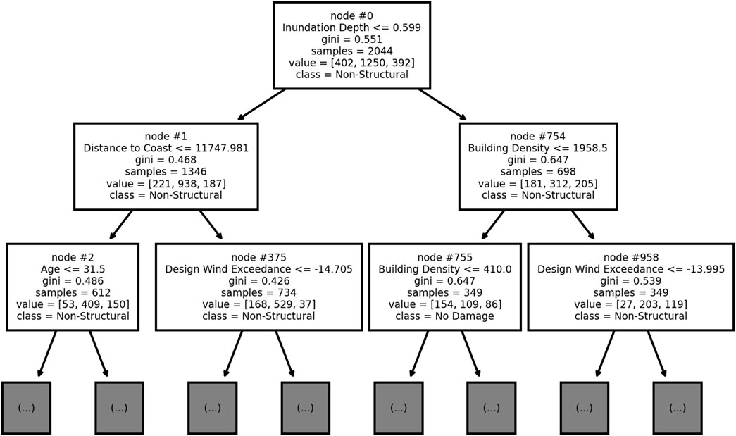
FIGURE 1. Partial decision tree for a random sample of hurricane reconnaissance data.

The feature space is split at specific values of individual features, creating what are called nodes, and the final groupings of observations when no further splits are made are called terminal nodes or leaves (James et al., 2013). The DT is fitted by making such splits to separate observations in the training data by class. A potential node can be parameterized by the feature, j (one of n features), that will be used to split the data, and the threshold, $t_m^j$, or value where the split will be made, and is defined as θ_m in Eq. 3.

${\theta }_m=\left(j,t_m^j\right)(3)$

where the subscript m is used to refer to a single node in the DT.

Looking at Node 0 (topmost box) in Figure 1, this node uses a threshold, $t_m^j$, of 0.599 for the feature, j, of Inundation Depth to separate observations based on their Inundation Depth value.

The result of a split at such a node is a collection of observations whose value of feature j fall below the threshold $t_m^j$ to the left of the node, and a collection of observations whose value for j exceed the threshold to the right following Eqs. 4, 5.

$Q_m^{\mathit{left}}\left({\theta }_m\right)=\left\{\left({\mathbf{x}}_i,y_i\right)\mid x_{i,j}\le t_m^j\right\},i=1,\dots ,l(4)$

$Q_m^{\mathit{right}}\left({\theta }_m\right)=\left\{Q_m\backslash Q_m^{\mathit{left}}\left({\theta }_m\right)\right\}(5)$

where Q_m is a set of observations (features and targets) entering node m, the term (x_i, y_i) represents a single observation (the vector of its feature values, x_i, and target value, y_i), x_i,j is the value of feature j in observation i, $Q_m^{\mathit{left}}$ is the subset of Q_m whose values for feature j fall below $t_m^j$ and are passed to the left of node m, and $Q_m^{\mathit{right}}$ is the subset whose values for j exceed $t_m^j$ and are passed to the right of node m.

Keeping with Node 0 in Figure 1, Q_m represents the set of (x, y) pairs for 2,044 observations in Node 0. $Q_m^{\mathit{left}}$ are the 1,346 observations whose Inundation Depth was below the threshold of 0.599 passed to Node 1 on the left, and $Q_m^{\mathit{right}}$ are the 698 observations whose Inundation Depth exceeded the threshold of 0.599 passed to Node 754 on the right.

Nodes are selected such that they reduce the downstream impurity to the left and right side of the node. A pure set of observations (impurity equal to zero) is the ideal case, in which all observations in the set have the same target class. Impurity then increases when a set contains observations with varying target classes. The selected node’s parameters, written as ${\theta }_m^{*}$, are chosen to minimize the total impurity, G, downstream of the split using the argument in Eq. 6.

${\theta }_m^{\ast }=\arg \underset{{\theta }_m}{\min }{G}_m\left(Q_m,{\theta }_m\right)(6)$

where G_m is the total impurity of node m, or the sum of the Gini index (defined in Eq. 8) on each side of the split weighted by the number of observations passed to each side, according to Eq. 7.

$G_m\left(Q_m,{\theta }_m\right)=\frac{q_m^{\mathit{left}}}{q_m}{H}_m^{\mathit{left}}\left(Q_m^{\mathit{left}}\left({\theta }_m\right)\right)+\frac{q_m^{\mathit{right}}}{q_m}{H}_m^{\mathit{right}}\left(Q_m^{\mathit{right}}\left({\theta }_m\right)\right)(7)$

where q_m is the number of observations entering node m, $q_m^{\mathit{left}}$ is the number of observations in $Q_m^{\mathit{left}}$, $q_m^{\mathit{right}}$ is the number of observations in $Q_m^{\mathit{right}}$, and H is the Gini index, the typical default impurity measure for DT algorithms.

In each node of Figure 1, the feature and threshold represent ${\theta }_m^{*}$, not any arbitrary θ_m, since only the selected nodes that satisfy Eq. 6 are shown in the DT output. For Node 0 in Figure 1, q_m is 2,044 (this differs from Q_m in that q_m is simply a count of observations, while Q_m is a set containing the observations’ features and targets). Node 1 contains $q_m^{\mathit{left}}$ and $H_m^{\mathit{left}}(Q_m^{\mathit{left}})$ as 1,346 and 0.468, respectively. Similarly, Node 754 contains $q_m^{\mathit{right}}$ and $H_m^{\mathit{right}}(Q_m^{\mathit{right}})$ as 698 and 0.647, respectively.

The Gini index, H, is a value that quantifies class impurity among a set of observations contained in a node, and is related to the proportion of each class represented in that node. Lower impurity aids correct predictions by demonstrating that the decision rules leading to that node sufficiently isolate a particular class. This value is calculated for Q_m in each node following Eq. 8.

$H_m\left(Q_m\right)=1-\sum _{s=1}^S{p}_{m,s}^2(8)$

where p_m,s is the proportion of observations in node m belonging to class s as determined by Eq. 9.

$p_{m,s}=\frac{1}{q_m}\sum _{y\in Q_m}\mathbf{1}\left(y=s\right)(9)$

where 1 is the indicator function yielding one if the argument is true and zero otherwise.

The p_m,s values for all S classes at any node m can be collected into a single vector, p_m, as in Eq. (10).

${\mathbf{p}}_m={\left[p_{m,1},p_{m,2},\dots ,p_{m,S}\right]}^T(10)$

From Figure 1, an example of p_m,s considering Node 1 and s = 1 would be 221 observations belonging to class 1 (first element in the “value” vector), divided by q_m = 1, 346 total observations in that node.

This process repeats for the subsets $Q_m^{\mathit{left}}({\theta }_m^{*})$ and $Q_m^{\mathit{right}}({\theta }_m^{*})$ contained on either side of the split until a user-defined maximum number of nodes have been created or until fewer observations remain than the user-defined number required for a new node to be created. Both of these stopping criteria are tunable hyperparameters, adjustable parameters which control the algorithm, and can be adjusted by the modeler. The probability of an observation belonging to a given target class is then the proportion of samples of that same class contained in its terminal node. The predicted class of an observation is determined as the class with the greatest probability as in Eq. 11.

$\text{DS}=\left(s\mid p_{M,s}=\max \left({\mathbf{p}}_M\right)\right)(11)$

where DS is the predicted damage state of an observation, and p_M,s is a component of vector p_M which is determined following Eq. 10 at the observation’s terminal node M.

After fitting the DT to training data, new (testing) data are sorted via the decision rules at the nodes in the DT, and their predicted classes determined according to Eq. 12.

$\text{DS}\left(\mathbf{u}\right)=f_{(\mathbf{x},\mathbf{y})}^{DT}\left(\mathbf{u}\right)(12)$

where $f_{(\mathbf{x},\mathbf{y})}^{DT}$ represents the decision rules of the DT defined by the parameters of all of its nodes (θ*) and fitted according to Eqs. 4 through 9, and outputs the predicted damage state of a testing observation following Eqs. 10, 11.

As an example of classifying new data with the DT, consider a testing observation with Inundation Depth = 0.25 and Distance to Coast = 15,000. Also assume that Figure 1 represents a complete DT instead of a partial one. This new data observation would start at Node 0 and be passed to the left to Node 1 since Inundation Depth of 0.25 is less than the threshold of 0.599. Next, since Distance to Coast of 15,000 exceeds the Node 1 threshold of 11,747.981, the observation would be passed to the right to Node 375. Assuming this is a complete DT, Node 375 would be a terminal node, and the observation would be classified as Non-Structural, determined by the majority of training observations in this node during fitting belonging to that class. The DT is desirable for its interpretability by simply examining feature and threshold values at each node and discerning whether an observation meets those thresholds.

3.2 Random forest

The RF model consists of an ensemble of DTs created as described in the previous section. Following RF formulation by Breiman (2001) and applications in Pedregosa et al. (2011), each DT in the RF ensemble is fit using a bootstrap, or subset, of training observations and considering only a subset of features when creating nodes in the DT. Fitting the underlying DTs in an RF on bootstraps of different observations and decorrelating those DTs by building them from differing sets of features reduce variance, or fluctuation in predictive accuracy given different testing data, thus making it robust to high dimensional data (Breiman, 2001). For a given testing observation, an RF algorithm sorts that observation through each DT in the RF, and averages the probabilistic class predictions from the output of the DTs to create a final prediction for that observation as the class with the highest probability. Figure 2 contains a flowchart depicting an ensemble of an arbitrary number r DTs being created from bootstraps of observations and subsets of input features, then testing data being input into those fitted DTs as indicated by the dashed box. While not as interpretable as a single DT, the RF is not a so-called “black box” algorithm since one could feasibly examine an observation’s path through each DT in the ensemble to analyze how the final prediction is made (James et al., 2013).

FIGURE 2

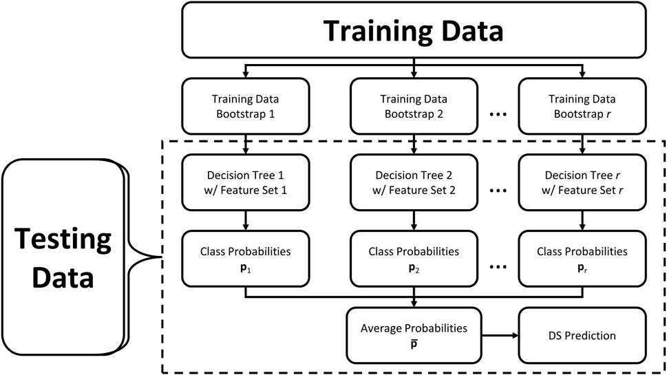
FIGURE 2. Flowchart of random forest procedure: training data is used in all steps to fit the model, then new (testing) data is classified using the steps indicated by the dashed box.

In context of this study, each DT in the RF ensemble maps observations’ features to class probabilities following Eq. 10 at terminal nodes. Then, the probabilities obtained from all DTs are averaged using Eq. 13.

$\bar{\mathbf{p}}=\frac{1}{R}\sum _{r=1}^R{\mathbf{p}}_{M,r}(13)$

where $\bar{\mathbf{p}}$ is the average class probability vector, and p_M,r is calculated by Eq. 10 for the terminal nodes, M, where an observation is sorted in each of R DTs in the RF ensemble.

Finally, an observation’s predicted damage state can be taken as the class with the greatest average probability as in Eq. 14.

$\text{DS}=\left(s\mid {\bar{p}}_s=\max \left(\bar{\mathbf{p}}\right)\right)(14)$

After all the DTs in the RF ensemble are fitted, a new (testing) observation can be classified by sorting it through each DT and averaging the resulting class probabilities, thus solving the problem statement of Eq. 1 by Eq. 15.

$\text{DS}\left(\mathbf{u}\right)=f_{\left(\mathbf{x},\mathbf{y}\right)}^{RF}\left(\mathbf{u}\right)(15)$

where $f_{(\mathbf{x},\mathbf{y})}^{RF}$ represents the RF ensemble of DTs fitted according to Eqs. 4 through 9 and outputs the predicted damage state of the testing observation following Eqs. 10, 13 and 14.

3.3 Additional algorithms investigated in this study

3.3.1 K-nearest neighbors

In addition to the RF and DT algorithms, KNN and GBC were also selected for investigation given their applicability to the dataset size, objective of classification, and nonlinear prediction mechanisms. The KNN algorithm is relatively simple compared to other nonlinear classification algorithms (Goldberger et al., 2004). The following algorithm overview was adapted from Pedregosa et al. (2011) which provides a common contemporary application of the KNN algorithm formulated by Fix and Hodges Jr (1951) and Altman (1992). A KNN model is fitted by simply plotting training data onto an n-dimensional coordinate system for n features, as presented in Figure 3 for an arbitrary two-feature example. When the training data are plotted, the target classes, shown as damage states, are known as represented by the symbology in Figure 3. Next, the testing data are similarly plotted, but without a known target class. A user-defined number, k, training observations, or neighbors, nearest a testing observation are used to predict the class for that testing observation, as identified in the figure. An observation’s predicted class is then determined by either a simple vote of the neighbors’ classes or a vote of the neighbors’ classes weighted by the inverse of their distance from the testing observation. Selecting the value for k typically involves an automated, iterative process of fitting the KNN with k values ranging from one through $\sqrt{n}$, as a rule of thumb, and selecting the value that yields the greatest accuracy (Hassanat et al., 2014). A weighting scheme is also typically selected in a similar manner. For target classes representing damage states as in Figure 3, the problem statement of Eq. 1 is satisfied by Eq. 16.

$\text{DS}\left(\mathbf{u}\right)=f_{\left(\mathbf{x},\mathbf{y}\right)}^{\mathit{KNN}}\left(\mathbf{u}\right)=\left(s\mid k_s=\max \left(\mathbf{k}\left(\mathbf{u},\mathbf{x},\mathbf{y}\right)\right)\right)(16)$

where $f_{(\mathbf{x},\mathbf{y})}^{\mathit{KNN}}(\mathbf{u})$ represents the operations of the KNN algorithm fitted to (x, y) to classify new data u, k (u, x, y) is a vector of length S for s = 1, … , S classes in the data where each element represents the count of k-neighbors belonging to each class (unweighted voting) or the sum of the k-neighbors belonging to each class multiplied by the inverses of their respective distances to u (distance-weighted voting).

FIGURE 3

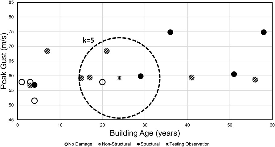
FIGURE 3. Example of k-nearest neighbors procedure using arbitrary data with two features and k = 5.

3.3.2 Gradient boosting classifier

Like an RF, a GBC is comprised of an ensemble of DTs to make predictions. In contrast to RF, GBC is built using regresssion DTs rather than classification DTs and instead of averaging the ensemble’s output, GBC uses sequential DTs, with each DT in the model fit to minimize a loss function of the ensemble’s output (Friedman, 2001). The following overview is adapted from GBC formulation by Friedman (2001, 2002) with applications specific to the multi-class (more than two target classes present in the data) GBC from Pedregosa et al. (2011).

In a multi-class GBC, separate DTs are created for each of S target classes in the data at a user-defined number, R, instances, so that the completed ensemble contains S × R DTs (Pedregosa et al., 2011). In the DT created for each class, training observations are assigned a “true label” of 1 if the observation belongs to that class and 0 otherwise. Each DT is then fitted to estimate these true labels, resulting in predicted labels which are the estimated probability that an observation belongs to the class the DT represents. A vector of predicted labels for training observations, p_r,s(x), is determined via Eq. 9 at the observations’ respective terminal nodes, M, in instance r for y ∈ {0, 1} respective to the class, s, represented by the DT.

Fitting in this manner creates decision rules in the DTs to minimize the total loss in the ensemble of predicted relative to true labels at each instance following Eq. 17.

$h_{r,s}\left(\mathbf{x},\mathbf{y}\right)=\arg \underset{h}{\min }{L}_{r,s}\left({\mathbf{y}}_s,{\mathbf{F}}_{r,s}\left(\mathbf{x}\right)\right)(17)$

where h_r,s (x, y) represents the DT for class s in instance r, L_r,s is the loss function for the class s ensemble through instance r, y_s is a vector containing observations’ binary true labels respective of class s, F_r,s(x) is the sum of all DT outputs p_r,s(x) for the class s ensemble through instance r. While a variety of differentiable loss functions have been proposed (Friedman, 2001, 2002), Eq. 18, which presents the log-loss, is a typical loss function for multi-class GBC (Friedman, 2001; Pedregosa et al., 2011).

$\begin{array}{c}\hfill L_{r,s}\left({\mathbf{y}}_s,{\mathbf{F}}_{r,s}\left(\mathbf{x}\right)\right)=\frac{1}{l}\sum _{i=1}^l\left(y_{s,i}\log \left(F_{r,s}\left({\mathbf{x}}_i\right)\right)+\left(1-y_{s,i}\right)\log \left(1-\left(F_{r,s}\left({\mathbf{x}}_i\right)\right)\right)\right)\end{array}(18)$

where y_s,i and F_r,s (x_i) are elements of vectors y_s and F_r,s(x), respectively, representing values for observation i. To minimize the loss function efficiently, Eq. 17 can be solved as a single parameter optimization where Eq. 18 is approximated via a first-order Taylor approximation (Friedman, 2001).

Additional DTs are fitted to the training data and added to the ensemble until a user-defined number, R, instances have been added to the ensemble, resulting in S separate solutions ${\mathbf{F}}_{R,s}(\mathbf{x})={\sum }_{r=1}^R{\mathbf{p}}_{r,s}(\mathbf{x})$. The separate solutions are combined into a single matrix, F_R(x) containing F_R,s(x) in the columns. Each row in this matrix representing an observation is then normalized via the softmax function, σ, defined in Eq. 19, to yield the probability that the observation belonging to each class.

$\mathit{\sigma }\left({\mathbf{x}}_i\right)=\frac{e^{{\mathbf{F}}_R\left({\mathbf{x}}_i\right)}}{{\sum }_{s=1}^S{e}^{F_{R,s}\left({\mathbf{x}}_i\right)}}(19)$

The predicted class for an observation is identified as that corresponding to the maximum probability, or highest value in the observation’s respective softmax vector σ(x_i). Thus, the problem statement of Eq. 1 can be solved in the context of a GBC by introducing new (testing) data into the GBC ensemble, sorting the data through each DT in the ensemble according to their feature values, u, and identifying the most probable class determined by the softmax function, as summarized in Eq. 20.

$\text{DS}\left(\mathbf{u}\right)=f_{\left(\mathbf{x},\mathbf{y}\right)}^{\mathit{GBC}}\left(\mathbf{u}\right)=\left(s\mid {\sigma }_s=\max \left(\mathit{\sigma }\left(\mathbf{u}\right)\right)\right)(20)$

where $f_{(\mathbf{x},\mathbf{y})}^{\mathit{GBC}}$ represents the decision rules of the GBC ensemble fitted to (x, y) and gives the predicted damage state of the testing observation as the class following Eqs. 17 through 20.

3.4 Performance metrics

Both accuracy and average f1-score were used as metrics to evaluate performance of the ML models, which are ubiquitous metrics in multi-class ML (e.g., Jeni et al., 2013; Grandini et al., 2020; Tharwat, 2020). Accuracy is a simple measure of overall correct predictions as in Eq. 21.

$Accuracy=\frac{\text{number\hspace{0.17em}of\hspace{0.17em}correct\hspace{0.17em}predictions}}{\text{total\hspace{0.17em}number\hspace{0.17em}of\hspace{0.17em}predictions}}(21)$

Average f1-score relies on two components - precision and recall - and gives a closer look at multi-class performance where one or more classes may be predicted more accurately than the others. A confusion matrix which plots true class labels against predicted class labels is a useful visual aid in interpreting these metrics. Precision and recall are both calculated for each class independently using the count of True Positives (TP), False Positives (FP), and False Negatives (FN) as depicted in the example confusion matrix in Figure 4 for the No Damage class. Using the example of the No Damage class, precision can be described as the rate of correct No Damage predictions out of all predictions of No Damage. Precision is evaluated using Eq. 22, written for any class s.

${Precision}_s=\frac{T{P}_s}{T{P}_s+F{P}_s}(22)$

FIGURE 4

FIGURE 4. Sample confusion matrix depicting True Positives in the dashed box and False Positives and False negatives in the left column and top row, respectively, excluding the dashed box, for the No Damage class.

Still using the No Damage class as an example, recall is described as the rate of correct No Damage predictions out of all observations whose true label is No Damage. Recall is calculated with Eq. 23, written for any class.

${Recall}_s=\frac{T{P}_s}{T{P}_s+F{N}_s}(23)$

The f1-score combines these two metrics as the harmonic mean of precision and recall, and is also calculated for each class independently following Eq. 24.

${f1-score}_s=2\times \frac{{Precision}_s\times {Recall}_s}{{Precision}_s+{Recall}_s}(24)$

The average f1-score, $\overline{f1}$, used as a metric in this study, is the mean of the f1-scores for all classes, calculated in Eq. 25.

$\overline{f1}=\frac{1}{S}\sum _{s=1}^S{f1-score}_s(25)$

4 Case study

The objective of this study’s ML framework is the ability to forecast building damage throughout an impact area on a building-by-building basis. The end user of such a model could be anyone from a homeowner to a regional or state entity with region-wide building data, investigating the risk of that region for an imminent or hypothetical hurricane. Before such a model can be used for forecasting, however, its performance needs to be tested on existing data as in a hindcast. In this case, input features consist of building characteristics, wind and surge hazard parameters, and geospatial data for buildings impacted by Hurricanes Harvey (2017), Irma (2017), Michael (2018), and Laura (2020). The target class for each observation is the damage state observed during reconnaissance efforts for each hurricane. These input and target variables, listed with their sources in Table 1, will be discussed in detail in the following subsections.

TABLE 1

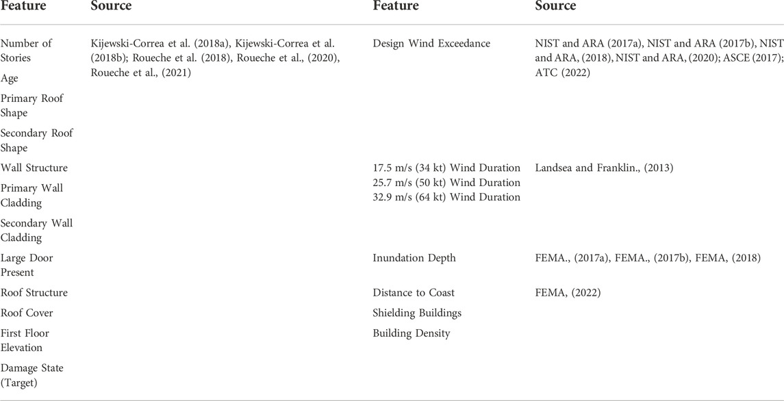
TABLE 1. List of all features considered in this study and their sources.

4.1 Building data

Since it is known that buildings of different age, materials, and geometry will perform differently when subjected to the same loading, it is imperative that these parameters are considered when predicting building damage. State-of-the-art models such as Hazus (FEMA, 2021a,b; Vickery et al., 2006a,b) use detailed building characteristics, each with experimentally derived load resistance, when developing building archetypes which are then subjected to loads calculated using hurricane intensity parameters. It is noted by Wu and Snaiki (2022) that “knowledge-enhanced machine learning,” which attempts to capture such underlying physics in a data-driven ML model, assists in efficiency and accuracy of ML models in wind engineering. Despite ML algorithms not directly calculating loading and resistance for building components, incorporating these building characteristics as variables aims to maintain the engineering factors at play when buildings are damaged by hurricane hazards. Thus, reconnaissance datasets containing building characteristics and their post-event damage states were examined. Hurricanes Harvey, Irma, Michael, and Laura were selected based on the availability of such extensive datasets published by the NSF-funded StEER and Geotechnical Extreme Events Reconnaissance (GEER) networks (Kijewski-Correa et al., 2018a; Kijewski-Correa et al., 2018b; Roueche et al., 2018, 2020, 2021). Combining these reconnaissance datasets resulted in 3,796 buildings, or observations, each with 11 building input features and the target damage state. Where “primary” and “secondary” are used in feature names in Table 1, for example with wall cladding, “primary” indicates the cladding material found on the majority of the building, while “secondary” refers to additional cladding materials on the building, if any.

The target here is a qualitative damage state that can take on one of three distinct classes for an observation: No Damage, Non-Structural Damage, and Structural Damage. These damage states were adapted from those of Vickery et al. (2006a), used in the original reconnaissance data and in Hazus, by combining the Minor and Moderate damage states into the Non-Structural Damage class, and combining Severe and Destruction into the Structural Damage class. These class descriptors are consistent with the types of damage associated with them as shown in Table 2. If any listed component of a building experienced a criterion of a higher damage state, the higher damage state was applied to that building. The 3,796 buildings’ locations and damage states are shown in the map of Figure 5. Buildings which contained insufficient data for ML analysis (see Section 4.3.1) are also identified in this map.

TABLE 2

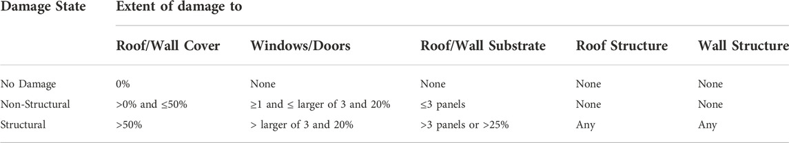
TABLE 2. Description of damage states in this study.

FIGURE 5

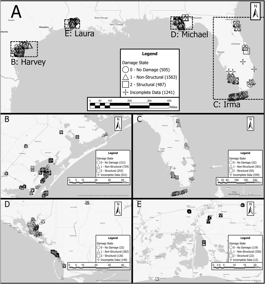
FIGURE 5. Map of buildings in the dataset and their damage states (A) Overview map of combined dataset (B) Hurricane Harvey in Texas (C) Hurricane Irma in Peninsular Florida (D) Hurricane Michael in the Florida Panhandle; and (E) Hurricane Laura in Louisiana.

4.2 Hazard and geospatial data

Hurricane hazard features were obtained for each observation in the reconnaissance datasets. Peak 3-s wind gust at 10 m height was obtained from National Institute of Standards and Technology (NIST) and Applied Research Associates’ (ARA) windfield map data (NIST and ARA, 2017a; b, 2018, 2020), consisting of grids of peak wind gust values interpolated from observation tower data. Since the design wind speed varies throughout the various hurricane impact regions, typically according to American Society of Civil Engineers (ASCE) Minimum Design Loads and Associated Criteria for Buildings and Other Structures, or ASCE 7, the peak wind gust values were not used as a feature. Instead, peak gust values were compared to the design wind speed for the zip code of each observation using Applied Technology Council (ATC, 2022) Hazards by Location tool (2022) with ASCE, (2017) Risk Category II design wind speeds. While the 2016 edition of ASCE 7 and Risk Category II do not apply to all observations in the dataset, these values were assumed to give a regional baseline for expected wind speeds and were used to create the input feature Design Exceedance.

The duration of sustained winds was also hypothesized to contribute to structural performance. To obtain these values, the storm track and wind speed radii tabulated in the National Hurricane Center (NHC) HURDAT2 dataset (Landsea and Franklin, 2013) were used to obtain the duration which each observation experienced 17.5 m/s (34 kt), 25.7 m/s (50 kt), and 32.9 m/s (64 kt) sustained wind speeds.

To capture the multi-hazard impacts on building performance, inundation depth at the location of each observation was determined from FEMA coastal surge depth grids for each hurricane. These grids were generated by FEMA and its affiliates using modeled inundation depth (determined by subtracting land surface digital elevation model from modeled water surface elevation) and validated according to observed peak inundation depths at observation stations throughout the impact areas (FEMA, 2017a; FEMA, 2017b, FEMA, 2018). In addition to inundation depth, three geospatial features which influence the effects of storm surge and wind loading on buildings were considered. Using geographic information system (GIS) software, the distance from each building to the coast was calculated as the minimum distance from the building’s footprint centroid to the nearest coastline point. Shielding refers to the number of buildings situated between a given building and the nearest coastline point which could mitigate wind and surge impacts. Shielding was then expanded upon by considering the building density in the area surrounding each building, which further influences wind, surge, and windborne debris impacts. FEMA (2022) United States Structures building footprints were used to obtain these three geospatial features.

4.3 Case study model selection

The ML approach to the objective of this work was performed using algorithms available from the Scikit-Learn library in Python (Pedregosa et al., 2011). With the ML algorithms investigated for the objective of this study, model selection involves tuning the model to provide the best performance on the available data. The methods described in this subsection are general and do not apply specifically to this case study. However, they are presented in the context of the case study as they will vary from one case to another depending on the data and objective. The following subsections focus on model selection for the RF model, however each of the KNN, DT, and GBC models underwent the same processes.

4.3.1 Preprocessing

ML frameworks begin with preprocessing the data, which consists of handling missing data and transforming the data to a format or range that is conducive to the algorithm at hand. In this case, observations with missing data were simply eliminated. This reduced the usable dataset to 2,555 observations. Attempts were made at imputing the missing data through ML regression strategies, but the results did not provide adequate confidence and missing data imputation was abandoned. Regarding data transformation, categorical features such as cladding materials and roof shape were first modified to ensure consistent labeling (e.g., “asphalt shingles” and “shingles, asphalt” given the same name), and then given ordinal values (i.e., 1, 2, … ). Since RF relies on a set of rules defined when fitting its underlying DTs, the range of values for individual features are insignificant, as opposed to proximity-based algorithms such as KNN or parametric algorithms like neural networks. As such, no scaling or normalization of the features were performed.

After preprocessing, the dataset was split into training and testing subsets. The training set is used to fit the model and create the decision rules for classifying observations. The testing set is kept separate until after the model is fitted, and then used to evaluate model performance on data that it has not “seen” yet. A random subset of 80% of the preprocessed data (2,044 observations) were used for training in a stratified fashion, maintaining the same proportion of each class as in the full dataset, and the remaining 20% (511 observations) were set aside for testing.

4.3.2 Model tuning

Next, feature selection was performed using the training set to determine which of the 19 features positively contribute to predictive accuracy. In lieu of an exhaustive, computationally expensive search of all combinations of features, forward and backward stagewise selection were performed. In stagewise selection, features are sequentially added (forward) or removed (backward) one at a time and selected such that the added or removed feature offers the greatest performance improvement as determined by accuracy and f1-scores obtained during 10-fold cross-validation (CV) until no further improvement is achieved. 10-fold CV involves splitting the training observations into 10 equal groups, training the model on 9 of the groups, evaluating on the remaining group, and repeating until each group has been used to evaluate the model. However, these feature selection methods offered negligible improvement compared to a model using all available features. Additionally, feature importance, measured as the Gini importance or the reduction in class impurity by splitting an individual feature, was calculated to identify an optimum subset of features. Using feature importance values as a starting point and engineering judgement for additional feature selection, six features were selected as the model input: Design Exceedance, Distance to Coast, Age, Inundation Depth, Building Density, and Roof Structure.

The training set was then used to select the hyperparameters for the RF model. Hyperparameters that were tuned for this RF model were the number of underlying DTs, the maximum number of features used to build each DT, and the minimum number of observations required to warrant a split in the DT. Hyperparameter tuning was performed using a grid search of ranges of hyperparameter values, in which an RF model was made with each possible combination of tunable hyperparameter values, and evaluated using 10-fold CV. The combination of hyperparameters that provided the best average performance was then selected for the model. The selected hyperparameters were 100 DTs, each built using two random features of the six selected features, and a minimum of seven observations required for a split to be made. All remaining hyperparameters available for the RF used Scikit-Learn’s RF classifier default values¹.

5 Results and variations of case study

5.1 Baseline case study hindcast results

The RF tuned as described in the previous section serves as the baseline model in the hindcast objective of the case study. This model represents forecasting conditions assuming available data includes all six features in the best subset determined during model selection.

The ML algorithms were tuned, fit to training data, then evaluated by introducing the testing set of data which was held out during model tuning and fitting. The comparative performance of the DT, RF, KNN, and GBC models are presented in Table 3. Table 3 also compares the computation time for each model, which includes hyperparameter tuning, fitting the tuned model, and classifying testing data. The computation times in Table 3 were obtained using 8-core multi-processing parallelism on 11th Gen Intel^® Core™ i7-11700 at 2.50 GHz. The DT was the least computationally expensive model, but a single DT proved to be too simple to capture trends in the testing data and produced the worst accuracy of 61%. The RF model produced the best accuracy of 76%, which was assisted by the fact that it includes many DTs, reducing variance and thus providing better estimations of unseen data in testing. The KNN, being a proximity-based algorithm, struggled to distinguish between different classes, which often overlapped in the feature space of the available data and gave 66% accuracy. Finally, the GBC, also an ensemble of DTs, performed nearly as well as the RF model at 72% accuracy, but with a larger computational expense and more hyperparameters to consider, proved to be overly sensitive to tuning without the benefit of increased performance.

TABLE 3

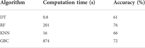
TABLE 3. Comparative performance and computation time (including hyperparameter tuning, fitting, and testing) for the classification algorithms considered in this study.

The overall accuracy of predictions by the selected RF model was 76%, with an average f1-score of 0.70. The confusion matrix of Figure 6 depicts these results. In this normalized confusion matrix, the values on the diagonals represent recall scores for their respective classes, which were 59.2% for No Damage, 87.5% for Non-Structural Damage, and 54.7% for Structural Damage. Weaker performance for the No Damage and Structural Damage classes was driven by class imbalance in the dataset. In both the training and testing sets, the Non-Structural Damage class contained three times as many samples as each of the other two classes. The impacts of such an imbalance are reflected by the lower average f1-score compared to accuracy, and are discussed in Section 6.

FIGURE 6

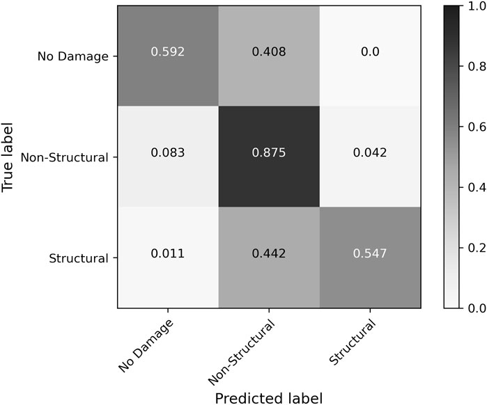
FIGURE 6. Normalized confusion matrix for baseline RF model predictions of testing data.

5.2 Dataset size sensitivity analysis

Since reconnaissance data containing the required level of detail for building features was limited to 3,796 observations, of which 2,555 were usable, a sensitivity analysis of sample size (number of observations) was also conducted. The impact of sample size has been documented by Cui and Gong (2018), who found that multiple ML regression algorithms exhibited exponential increase in prediction accuracy as a function of sample size. Sordo and Zeng (2005) similarly demonstrated such increase in accuracy for 3 ML classification algorithms, including tree-based algorithms. To evaluate the effect of sample size on damage state prediction accuracy in this study, data from each hurricane was sequentially tested in the order they occurred: Harvey, Irma, Michael, then Laura. At each step in this sequential prediction study, all the data from hurricanes prior to and including that step were shuffled, 80% of the data were used to fit the model, and the remaining 20% of data were used to test performance. The results shown in Figure 7 depict generally linear increasing trends in performance metrics, with the exception of average f1-score in the second step of the sequential process. The dip in average f1-score for this step, containing Harvey and Irma data, resulted again from poorer recall of the underrepresented No Damage and Structural Damage classes of 47.9% and 49.2%, respectively, compared to 82.5% recall for the Non-Structural Damage class.

FIGURE 7

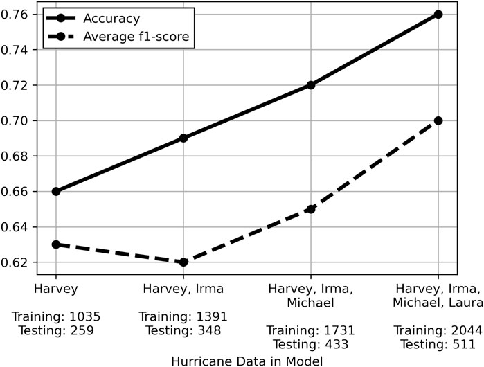
FIGURE 7. Performance of random forest model using sequentially added hurricane data.

5.3 Parametric studies of input features

During forecasting, hazard features will be obtained from modeling by other researchers and organizations as hurricanes begin to develop. Depending on the resolution of available modeling for a hurricane, inundation depths may not be available for forecasting since propagating wave and surge impacts onto land requires high grid resolution. Geospatial features are typically readily attainable since FEMA and others have building footprint datasets for nearly all buildings in the United States. Building data, however, which are typically obtained from county property appraisal offices, are sometimes sparse and vary greatly depending on the study region. With these potential forecasting limitations in mind, parametric studies considering availability of different features were generated as described in Table 4.

TABLE 4

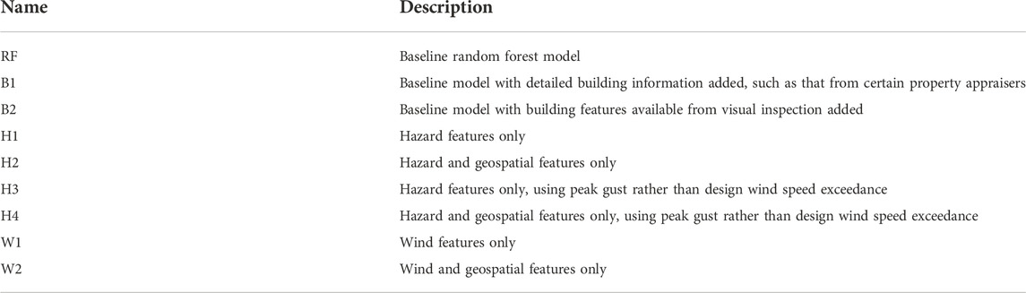
TABLE 4. Parametric study descriptions.

In Table 4, RF denotes the baseline RF model of this study, trained on the six features selected during model selection. Input features were then modified in the “building” cases, denoted as B-, to represent availability of different building features. The Bay County, Florida Property Appraiser is an example of one of the more robust building data sources, listing such data for each building as age, framing type, wall cladding, roof cover, and footprint area. Conversely, in rural communities such information is often unavailable, as is the case with Plaquemines Parish, Louisiana, which simply lists the occupancy type. With this consideration in mind, two levels of detail for building data were considered as supplementary features to the baseline model: B1 which allows for more detailed information as listed for Bay County, Florida, and B2 which considers building features available from a visual inspection. Visual inspections could potentially be performed with door-to-door inspections of a study region, or using emerging artificial intelligence (AI) technology such as Building Recognition using AI at Large Scale (BRAILS) to collect this information by processing street-view imagery with ML (Wang et al., 2021).

Other models were considered with the understanding that building data may not be rapidly available as hurricanes approach, as mentioned for rural regions particularly. These “hazard” analyses, denoted as H- in the test matrix, consider the absence of building features and availability of only wind and inundation hazard features with and without geospatial features. Additionally, separate analyses were performed to compare design wind speed exceedance as a feature (as was used in the baseline model) with using peak gust values instead, without consideration of design wind speed.

Finally, forecasting cases in which hurricane modeling grid resolution is such that inland inundation cannot be determined were considered. “Wind” models were created using a W- designation which consider only wind-related features being available, both with and without accompanying geospatial features.

For each of these parametric studies, the full list of features corresponding to the case description were used as input. Since these models each consider a small number of features, an exhaustive search of feature combinations was feasible to determine the best subset of features for each model. This process, called best subset selection, evaluates performance of the model using each combination of features and results in a model trained only on the combination that yields the best accuracy.

Performance of the various parametric models as well as the list of features considered and those selected for each are given in Table 5. As expected, the B1 model which considered all the baseline RF features plus additional building features, ultimately used only the features of the baseline RF model and resulted in the same performance. B2, which excluded the building features of the baseline RF, reduced accuracy by 5.3%. The absence of critical building data (age and roof structure) was not counterbalanced by less influential building characteristics considered in the B2 model.

TABLE 5

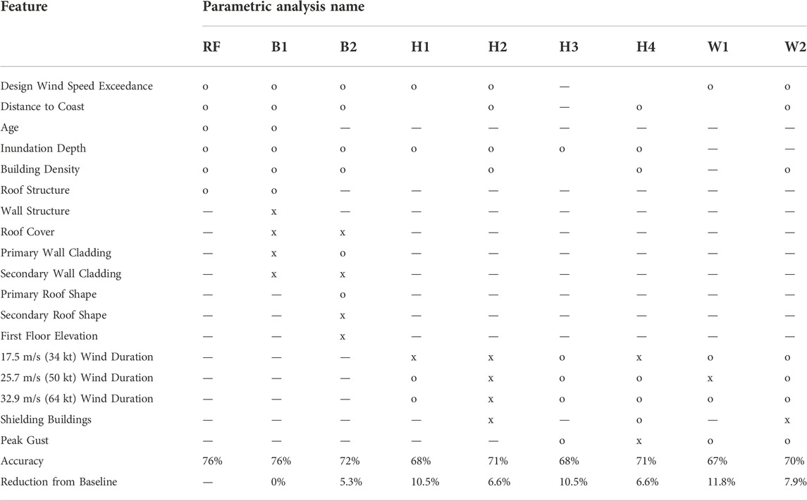
TABLE 5. Parametric study test matrix, where “o” indicates a feature was included in the selected features for a model, and “x” indicates a feature was considered but not selected for the model.

While using different subsets of hazard features, H2 and H4, which consider geospatial features, performed considerably better (6.6% accuracy reduction) than H1 and H3 which used hazard features only and excluded geospatial features (10.5% accuracy reduction). Likewise in the “wind” models, inclusion of geospatial features benefits the W- models. Still, without inclusion of more influential building features and consideration of storm surge effects, these models performed worst of all those in the study with 11.8% and 7.9% accuracy reduction in W1 and W2, respectively.

5.4 Comparison to Hazus predictions

FEMA’s Hazus software (FEMA, 2021a, FEMA, 2021b; Vickery et al., 2006a, Vickery et al., 2006b) is widely used in hurricane hazard engineering applications to estimate damage and economic loss from hurricanes. This software provides a comprehensive approach to modeling wind, storm surge inundation, and windborne debris intensity based on hurricane track parameters. Since Hazus is well-established in the hazard engineering community and is built upon engineering theory and extensive experimental testing, it was selected as a baseline against which ML damage predictions could be compared. Furthermore, the damage states predicted by the RF model were selected such that they correspond with Hazus damage states as such: No Damage is equivalent to Hazus DS-0, Non-Structural Damage refers to Hazus DS-1 and DS-2, and Structural Damage encompasses Hazus DS-3 and DS-4.

The analysis follows Hazus’s Level 2 analysis, which uses observed hurricane track and wind parameters included in the software package to determine hazard intensities, and applies the resulting forces to user-defined buildings which contain data about the buildings’ location, age, footprint area, occupancy type, and building type (FEMA, 2021a). Hazus calculates loads imparted on buildings by generating wind speed profiles based on peak wind gusts and aggregated to a single value per Census tract (Vickery et al., 2006b; FEMA, 2021a). Building damage is then determined from applying calculated pressures and impact loading onto building models representing occupancy and building types, iteratively checking for damage based on experimentally derived resistance values of components in the assumed building models and recalculating loads imparted on the building models as damage occurs (Vickery et al., 2006a; FEMA, 2021b).

The user-defined buildings input into Hazus analyses were the same buildings from the testing data in the RF model, which were assigned occupancy and building types according to definitions in Hazus documentation. Each of the hurricanes in the study was applied in Hazus to the input buildings respective of that hurricane, and damage state probabilities were returned. For each building, the damage state with the highest probability was the Hazus prediction for that building, and the Hazus damage state was converted to the damage state scheme of the case study ML framework.

To evaluate the validity of this comparison, peak wind gust and maximum sustained wind speed used by Hazus for estimating pressures acting on building components were compared to values from NIST/ARA datasets used in the ML framework. Since Hazus uses wind speed parameters aggregated at the Census tract level, the grids of peak gusts and sustained wind speeds in the NIST/ARA data were averaged throughout each Census tract. Both of these parameters demonstrated strong agreement between Hazus values and averaged NIST/ARA data values as shown in Figure 8. Agreement between the two sources is indicated by an R² value of 0.97 and mean absolute error (MAE) of 0.96 m/s for peak gusts and an R² value of 0.95 and MAE of 0.93 m/s for maximum sustained wind speeds.

FIGURE 8

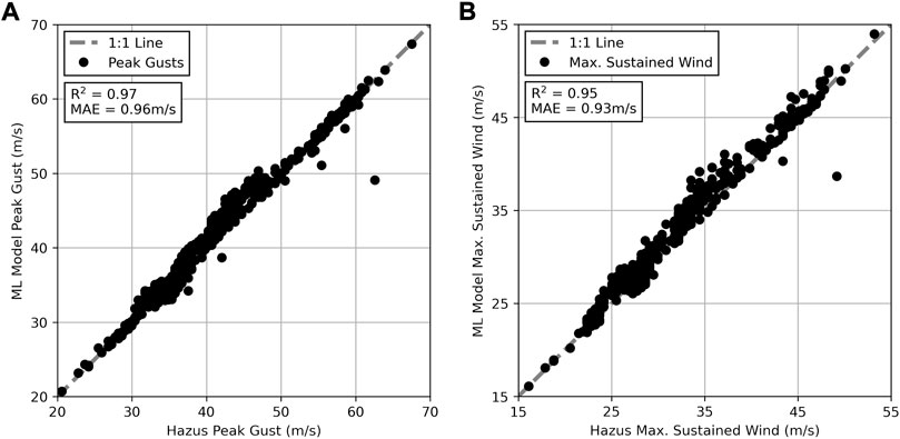
FIGURE 8. (A) Comparison of Hazus peak gust and peak gusts from NIST/ARA data used in ML framework, aggregated at Census tract level (B) Comparison of Hazus maximum sustained wind speeds and those from NIST/ARA data used in ML framework, aggregated at Census tract level.

Finally, the sequential prediction methodology used for the RF model was also applied to Hazus predictions to observe trends in performance when applied to more scenarios. It was assumed that this computational model based on probabilistic loads and resistances and application of engineering theory would not be impacted by sequential analyses since it uses direct calculations to determine damage states, rather than learned trends as in the RF model.

Subjecting the buildings represented in the testing data to their respective hurricanes using Level 2 Hazus analysis with user-defined buildings resulted in 47% overall accuracy, with an average f1-score of 0.35. These results are not indicative of Hazus’ predictive capacity as a whole, since the tool is intended for decision support on “state, local, tribal, and territorial” scales (FEMA, 2021a). Instead, they highlight potential limitations in building-level predictions by Hazus, which others have attributed to deviations in building type distribution among user-defined facilities relative to aggregated stock building inventory (Hernandez, 2020). The Hazus model had a strong tendency to misclassify buildings as Non-Structural Damage (Hazus DS-1 and DS-2) as shown in the confusion matrix of Figure 9. From this confusion matrix, it is clear that the majority of Structural Damage observations were misclassified as Non-Structural Damage, as were more than half of the No Damage observations. These results coincide with those of Subramanian et al. (2013) who observed Hazus predictions of roof damage (one component considered when ascribing damage states) to over 700,000 buildings from Hurricane Ike in Harris County, Texas with only 29.5% accuracy due to both over- and under-predictions. Since their study only analyzed roof damage, predictions were considered accurate if the observed and predicted roof damage ratios were consistent with the same damage state. Furthermore, Subramanian et al. (2013) similarly employed an ML ensemble of DTs for comparison and found greatly improved predictive accuracy of 86% when testing on 90% of the Harris County Hurricane Ike data.

FIGURE 9

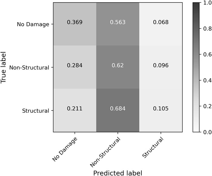
FIGURE 9. Normalized confusion matrix of Hazus predictions of buildings in testing data of baseline RF model.

Employing the sequential prediction methodology in Hazus involved performing each hurricane analysis independently and sequentially combining the results. As indicated in Figure 10, Hazus performance generally did not fluctuate with the number of observations. This is expected since Hazus does not rely on additional data for training. Instead, it compounds probabalistic component resistance of detailed building archetype models and probabilistic loading from wind speed parameters to calculate estimated damage. Given the explicit calculations of the Hazus model, it is expected that not much variance should occur in the accuracy across multiple events or building types.

FIGURE 10

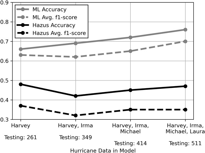
FIGURE 10. Hazus performance compared to random forest model using sequentially added hurricane data.

6 Discussion

6.1 RF model performance

While the R² values typically evaluated in regression models cannot be directly compared to the 76% predictive accuracy of the classification model developed in this study, the relative performance of each type of model gives insights into important damage prediction features. The regression models of Szczyrba et al. (2020) to predict hurricane damage ratios at the census tract level, and Wendler-Bosco and Nicholson (2021) to predict county-wide damage ratios and aggregate them throughout the entire impact were able to capture 29% and 50–60% of the variance in observed damage ratios (R² values), respectively. The RF model of this study benefited from a comparatively more holistic range of features which was not limited to hurricane parameters, but also considered building features which contribute to load-resisting capacity of buildings and geospatial features which influence load mitigating effects of nearby buildings and breakdown of hazard intensity as a storm moves inland. The work of Szczyrba et al. (2020), particularly, does offer insight for future work, as they note in their work and their references that social and demographic features are highly correlated to the extent of damage in extreme events. Such features were not considered in the present study, but could prove beneficial going forward.

The classification model of van Verseveld et al. (2015), which states prediction accuracy of each class and uses a different damage rating scheme, also does not provide a direct comparison to accuracy of the RF model developed in this study, but does follow similar trends at the class level. Their Bayesian network provided 68.4% and 95.8% correct classification for “affected” and “minor” damage states, but less than 5% for higher damage states. Their “affected” and “minor” damage states can be most closely compared to the Non-Structural Damage class of the present study, which was predicted correctly in 87.5% of cases (recall). Performance of the higher damage state of the Structural Damage class similarly waned as the worst-performing class in this study, with 54.7% of cases correctly recalled. In this case, better performance of the Non-Structural Damage class is likely driven by an imbalance toward this class in the available data. The No Damage and Structural Damage classes each contained only one-third of the number of observations in the Non-Structural Damage class. Since more majority class observations are available to offer greater proportions in terminal nodes, such an imbalance leads to better reinforcement of decision rules to classify the majority class and lesser influence of minority class observations. Oversampling and undersampling methods including random over- and undersampling and the Imbalanced Learn synthetic minority oversampling technique (SMOTE) and near-miss undersampling algorithms (Lemaître et al., 2017) were employed to artificially balance class representation in the training data. These methods were sometimes effective in increasing minority class performance, but at the expense of Non-Structural class performance to the extent that accuracy and average f1-scores were reduced. To overcome the challenges of imbalanced data inherent with ML drawing from reconnaissance data, these strategies warrant further investigation in future work.

6.2 Reconnaissance data

The results of the sample size sensitivity analysis indicate a clear linear trend of improved performance given more observations from a greater number of hurricanes. Robust reconnaissance missions following future hurricanes will be vital in improving the damage prediction abilities of ML models by allowing for better learning, or greater reinforcement, of the factors associated with each damage state. The model in this study incorporates two building features for optimum performance: age and roof structure. These are two features that cannot be discerned from imagery and may not be available from public records, depending on the municipality. In the strenuous task that is hurricane reconnaissance, the effort of collecting these data can increase damage forecasting potential by over 5% as shown in the comparison to the B2 case of Table 5 which considers only externally visible building features. While additional building features, as in case B1, did not bolster predictive accuracy, it should not be assumed that theses features are not necessary in reconnaissance data collection. Instead, it is possible that as more data is collected on these features, their variance relative to damage state may become more adequately captured, increasing their influence in predictions.

6.3 Forecasting

Even with extensive datasets containing the optimum subset of features for this model in hindcast, forecasting may be limited depending on available data for the anticipated impact region. As shown by the H- and W- models in the parametric studies, decreasing fidelity results in decreasing predictive accuracy. Forecasting accuracy, regardless of additional reconnaissance data for training, will rely upon identifying attainable building features in an expected impact area and useful hazard features from hurricane modeling. Regarding building features, work is underway to collect bulk data from county-wide sources such as property appraisers, particularly in Florida. As noted in Section 5.3, these data may not contain all the necessary input features for the RF. One solution is to simply use the features that are available, which was demonstrated to reduce accuracy through parametric studies. An alternative is to restructure the input and re-frame the target such that it more closely follows the Hazus methodology of aggregated building data and damage predictions at a regional level. This would require much manipulation of the model, but is a worthy future objective to accommodate for a lack of building data or desire for building-level predictions.

To further increase forecasting ability, hazard features must be addressed as well. Terrain models exist, such as that in the Hazus model, which can be used to obtain the surface roughness coefficient, a factor in wind-related structural engineering which may prove to enhance similar features such as building density and distance to the coast. Further enhancements may be made by incorporating a broader range of water hazards. In the work of van Verseveld et al. (2015), wave attack, flow velocity, and scour depth were considered in addition to inundation depth, which was the only surge-related feature in the RF of this study. Generating new features to reflect interactions between existing hazard features, as employed by Massarra et al. (2020), may also provide improvements as a different approach to modeling the combined impacts of certain features. While additional features do not always lead to better accuracy, as demonstrated in the parametric studies, these features which address known engineering concepts could lessen the accuracy reduction observed when building data is limited.

7 Conclusion

A novel ML framework was developed using building, hazard, and geospatial features to predict building-level damage in three qualitative classes: No Damage, Non-Structural Damage, and Structural Damage. Performance of different algorithms has been investigated including KNN, DT, RF, and GBC algorithms. The RF model, selected for further analysis based on its performance and interpretability, was used to hindcast a sample of 511 buildings from Hurricanes Harvey, Irma, Michael, and Laura with 76% accuracy. The Non-Structural Damage class out-performed the other two classes by nearly 30% due to the imbalance in available data skewed toward Non-Structural observations. This could potentially be corrected using over- and undersampling techniques, but such progress has not been observed to date. It was also demonstrated that a greater number of observations from a variety of hurricanes and impact regions produces a linear trend of increasing accuracy. Parametric studies were performed to estimate forecasting abilities given availability of different features, which demonstrated that building data are required for optimum performance, both wind and inundation data are needed regarding hazard features, and geospatial features greatly contribute to accuracy of building-level predictions. It is particularly noted that the building features required for optimum performance relate to age and structural materials - two features that may not be publicly available, and cannot be supplemented via visual inspection or AI feature recognition. Finally, a comparison was made to predictions for the same set of buildings using FEMA’s Hazus Multi-Hazard Hurricane model, which yielded 47% accuracy, but offered insights into alternatives for forecasting given the variability of rapidly available data used in the ML framework as presented. Given the relatively high accuracy of the damage prediction model of this study, this model serves as a vital step in estimating community-wide risk at the building level from impending hurricanes - a resource that is ever more important as climate change and urbanization trends leave more buildings and more people in the path of increasing hurricane intensity and frequency.

Data availability statement

The original contributions presented in the study are included in the article/supplementary material, further inquiries can be directed to the corresponding author.

Author contributions

All authors contributed to conception and design of the study. SK organized the data, performed the presented analyses, and prepared the manuscript drafts with feedback and guidance from AS and MO. AS and MO additionally advised the model improvement approaches and results interpretation. All authors approved the manuscript for publication.

Funding

This research is supported by the National Oceanographic Partnership Program (Project Grant N00014-21-1-2203) and the University of Florida. This support is gratefully acknowledged.

Acknowledgments

The authors would like to acknowledge NSF-funded Natural Hazard Engineering Research Infrastructure (NHERI) DesignSafe which hosts the majority of data used in this study and the Structural Extreme Events Reconnaissance (StEER) network which offered details regarding the reconnaissance data production.

Conflict of interest

The authors declare that the research was conducted in the absence of any commercial or financial relationships that could be construed as a potential conflict of interest.

Publisher’s note

All claims expressed in this article are solely those of the authors and do not necessarily represent those of their affiliated organizations, or those of the publisher, the editors and the reviewers. Any product that may be evaluated in this article, or claim that may be made by its manufacturer, is not guaranteed or endorsed by the publisher.

Footnotes

¹https://scikit-learn.org/stable/modules/generated/sklearn.ensemble.RandomForestClassifier.html

References

Altman, N. S. (1992). An introduction to kernel and nearest-neighbor nonparametric regression. Am. Statistician 46, 175–185. doi:10.2307/2685209

CrossRef Full Text | Google Scholar

ASCE (2017). Minimum design loads and associated criteria for buildings and other structures. Am. Soc. Civ. Eng. 16, 7. doi:10.1061/9780784414248

CrossRef Full Text | Google Scholar

ATC (2022). Hazards by location.

Google Scholar

Berke, P., Larsen, T., and Ruch, C. (1984). A computer system for hurricane hazard assessment. Comput. Environ. Urban Syst. 9, 259–269. doi:10.1016/0198-9715(84)90026-7

CrossRef Full Text | Google Scholar

Breiman, L., Friedman, J., Stone, C., and Olshen, R. (1984). Classification and regression trees. Raton, FL: Chapman and Hall.

Google Scholar

Breiman, L. (2001). Random forests. Mach. Learn. 45, 5–32. doi:10.1023/a:1010933404324

CrossRef Full Text | Google Scholar

Calton, L., and Wei, Z. (2022). Using artificial neural network models to assess hurricane damage through transfer learning. Appl. Sci. 12, 1466. doi:10.3390/app12031466

CrossRef Full Text | Google Scholar

Cohen, D. T. (2018). Coastline county population continues to grow. Suitland: US Census Bureau.

Google Scholar

Cui, Z., and Gong, G. (2018). The effect of machine learning regression algorithms and sample size on individualized behavioral prediction with functional connectivity features. NeuroImage 178, 622–637. doi:10.1016/j.neuroimage.2018.06.001

PubMed Abstract | CrossRef Full Text | Google Scholar

FEMA (1992). Building performance: Hurricane andrew in Florida. Washington, DC: Federal Emergency Management Agency

Google Scholar

FEMA (2021a). Hazus-mh 4.2 hurricane model technical manual. Washington, DC: Federal Emergency Management Agency

Google Scholar

FEMA (2021b). Hazus-mh 4.2 inventory technical manual. Washington, DC: Federal Emergency Management Agency

Google Scholar

FEMA (2017a). Hurricane harvey fema coastal surge depth grid. Washington, DC: Federal Emergency Management Agency

Google Scholar

FEMA (2017b). Hurricane irma fema coastal surge depth grid. Washington, DC: Federal Emergency Management Agency

Google Scholar

FEMA (2018). Hurricane michael preliminary fema coastal surge depth grid. Washington, DC: Federal Emergency Management Agency

Google Scholar

FEMA (2022). USA structures. Washington, DC: Federal Emergency Management Agency

Google Scholar

Fix, E., and Hodges, J. (1951). Discriminatory analysis: Nonparametric discrimination: Consistency properties. Report No. 4. Texas: USAF School of Aviation MedicineRandolph Field. doi:10.2307/1403797

CrossRef Full Text | Google Scholar

Friedman, J. H. (2001). Greedy function approximation: A gradient boosting machine. Ann. statistics, 1189–1232.

CrossRef Full Text | Google Scholar

Friedman, J. H. (2002). Stochastic gradient boosting. Comput. statistics data analysis 38, 367–378. doi:10.1016/s0167-9473(01)00065-2

CrossRef Full Text | Google Scholar

Goldberger, J., Hinton, G. E., Roweis, S., and Salakhutdinov, R. R. (2004). Neighbourhood components analysis. Adv. neural Inf. Process. Syst. 17.

Google Scholar

Grandini, M., Bagli, E., and Visani, G. (2020). Metrics for multi-class classification: An overview. arXiv preprint arXiv:2008.05756

Google Scholar

Hao, H., and Wang, Y. (2019). “Hurricane damage assessment with multi-, crowd-sourced image data: A case study of hurricane irma in the city of miami,” in Proceedings of the 17th international conference on information system for crisis response and management (Valencia, Spain: ISCRAM), 19–22.

Google Scholar

Hassanat, A. B., Abbadi, M. A., Altarawneh, G. A., and Alhasanat, A. A. (2014). Solving the problem of the k parameter in the knn classifier using an ensemble learning approach. doi:10.48550/ARXIV.1409.0919

CrossRef Full Text | Google Scholar

Hernandez, N. (2020). An analysis of a hurricane loss model, validation from tyndall afb, and applications for the air force. Wright-Patterson Air Force Base, Ohio; Air Force Institute of Technology

Google Scholar

James, G., Witten, D., Hastie, T., and Tibshirani, R. (2013). An introduction to statistical learning, 112. Springer.

Google Scholar

Jeni, L. A., Cohn, J. F., and De La Torre, F. (2013). “Facing imbalanced data–recommendations for the use of performance metrics,” in 2013 Humaine association conference on affective computing and intelligent interaction, 2015 Jan 6. (IEEE), 245–251. doi:10.1109/ACII.2013.47

PubMed Abstract | CrossRef Full Text | Google Scholar

Kaur, S., Gupta, S., Singh, S., Koundal, D., and Zaguia, A. (2022). Convolutional neural network based hurricane damage detection using satellite images. Soft Comput. 26, 7831–7845. doi:10.1007/s00500-022-06805-6

CrossRef Full Text | Google Scholar

Kijewski-Correa, T., Gong, J., Womble, A., Kennedy, A., Cai, S. C., Cleary, J., et al. (2018a). Hurricane harvey (Texas) supplement – collaborative research: Geotechnical extreme events reconnaissance (geer) association: Turning disaster into knowledge. doi:10.17603/DS2Q38J

CrossRef Full Text | Google Scholar

Kijewski-Correa, T., Roueche, D., Pinelli, J.-P., Prevatt, D., Zisis, I., Gurley, K., et al. (2018b). Rapid: A coordinated structural engineering response to hurricane irma. florida. doi:10.17603/DS2TX0C

CrossRef Full Text | Google Scholar

Knutson, T., Camargo, S. J., Chan, J. C. L., Emanuel, K., Ho, C.-H., Kossin, J., et al. (2020). Tropical cyclones and climate change assessment: Part II: Projected response to anthropogenic warming. Bull. Am. Meteorol. Soc. 101, E303–E322. doi:10.1175/bams-d-18-0194.1

CrossRef Full Text | Google Scholar

Landsea, C. W., and Franklin, J. L. (2013). Atlantic hurricane database uncertainty and presentation of a new database format. Mon. Weather Rev. 141, 3576–3592. doi:10.1175/mwr-d-12-00254.1

CrossRef Full Text | Google Scholar

Lemaître, G., Nogueira, F., and Aridas, C. K. (2017). Imbalanced-learn: A python toolbox to tackle the curse of imbalanced datasets in machine learning. J. Mach. Learn. Res. 18, 1–5.

Google Scholar

Levin, E. L., and Murakami, H. (2019). Impact of anthropogenic climate change on United States major hurricane landfall frequency. J. Mar. Sci. Eng. 7, 135. doi:10.3390/jmse7050135

CrossRef Full Text | Google Scholar

Li, Y., Hu, W., Dong, H., and Zhang, X. (2019). Building damage detection from post-event aerial imagery using single shot multibox detector. Appl. Sci. 9, 1128. doi:10.3390/app9061128

CrossRef Full Text | Google Scholar

Marsooli, R., Jamous, M., and Miller, J. K. (2021). Climate change impacts on wind waves generated by major tropical cyclones off the coast of New Jersey, USA. Front. Built Environ. 7. doi:10.3389/fbuil.2021.774084

CrossRef Full Text | Google Scholar

Masoomi, H., van de Lindt, J. W., Ameri, M. R., Do, T. Q., and Webb, B. M. (2019). Combined wind-wave-surge hurricane-induced damage prediction for buildings. J. Struct. Eng. (N. Y. N. Y). 145. doi:10.1061/(asce)st.1943-541x.0002241

CrossRef Full Text | Google Scholar

Massarra, C. C., Friedland, C. J., Marx, B. D., and Dietrich, J. C. (2020). Multihazard hurricane fragility model for wood structure homes considering hazard parameters and building attributes interaction. Front. Built Environ. 6. doi:10.3389/fbuil.2020.00147

CrossRef Full Text | Google Scholar

Mitsuta, Y. (1996). “A predicting method of typhoon wind damages,” in Proc. Of ASCE specialty conference on probabilistic and structural reliability (Worcester, 970. –973.

Google Scholar

Mohleji, S., and Pielke, R. (2014). Reconciliation of trends in global and regional economic losses from weather events: 1980-2008. Nat. Hazards Rev. 15, 04014009. doi:10.1061/(ASCE)NH.1527-6996.0000141

CrossRef Full Text | Google Scholar

NIST and ARA (2017a). Hurricane harvey rapid response windfield estimate. Albuquerque, NM: Applied Research Associates

Google Scholar

NIST and ARA (2017b). Hurricane irma rapid response windfield estimate. Albuquerque, NM: Applied Research Associates

Google Scholar

NIST and ARA (2020). Hurricane laura rapid response windfield estimate. Albuquerque, NM: Applied Research Associates

Google Scholar

NIST and ARA (2018). Hurricane michael rapid response windfield estimate. Albuquerque, NM: Applied Research Associates

Google Scholar

Pedregosa, F., Varoquaux, G., Gramfort, A., Michel, V., Thirion, B., Grisel, O., et al. (2011). Scikit-learn: Machine learning in Python. J. Mach. Learn. Res. 12, 2825–2830.

Google Scholar

Pinelli, J.-P., Simiu, E., Gurley, K., Subramanian, C., Zhang, L., Cope, A., et al. (2004). Hurricane damage prediction model for residential structures. J. Struct. Eng. (N. Y. N. Y). 130, 1685–1691. doi:10.1061/(asce)0733-9445(2004)130:11(1685)

CrossRef Full Text | Google Scholar

Pita, G., Pinelli, J.-P., Gurley, K., and Mitrani-Reiser, J. (2015). State of the art of hurricane vulnerability estimation methods: A review. Nat. Hazards Rev. 16. doi:10.1061/(asce)nh.1527-6996.0000153

CrossRef Full Text | Google Scholar

Roueche, D. B., Lombardo, F. T., Krupar, Richard J., and Smith, D. J. (2018). Collection of perishable data on wind- and surge-induced residential building damage during hurricane harvey. doi:10.17603/DS2DX22

CrossRef Full Text | Google Scholar

Roueche, D., Kameshwar, S., Vorce, M., Kijewski-Correa, T., Marshall, J., Mashrur, N., et al. (2021). Field assessment structural teams: Fast-1, fast-2. fast-3. doi:10.17603/DS2-DHA4-G845

CrossRef Full Text | Google Scholar

Roueche, D., Kijewski-Correa, T., Cleary, J., Gurley, K., Marshall, J., Pinelli, J.-P., et al. (2020). Steer field assessment structural team (fast). doi:10.17603/DS2-5AEJ-E227

CrossRef Full Text | Google Scholar

Sordo, M., and Zeng, Q. (2005). On sample size and classification accuracy: A performance comparison. Biol. Med. Data Analysis, 193–201. doi:10.1007/11573067_20

CrossRef Full Text | Google Scholar

Subramanian, D., Salazar, J., Duenas-Osorio, L., and Stein, R. (2013). Constructing and validating geographically refined hazus-mh4 hurricane wind risk models: A machine learning approach. Adv. Hurric. Eng. Learn. our past, 1056–1066.

CrossRef Full Text | Google Scholar

Szczyrba, L., Zhang, Y., Pamukcu, D., and Eroglu, D. I. (2020). “A machine learning method to quantify the role of vulnerability in hurricane damage,” in ISCRAM 2020 conference proceedings–17th international conference on information systems for crisis response and management.

Google Scholar

Tharwat, A. (2020). Classification assessment methods. Appl. Comput. Inf. 17, 168–192. doi:10.1016/j.aci.2018.08.003

CrossRef Full Text | Google Scholar

van Verseveld, H. C. W., van Dongeren, A. R., Plant, N. G., Jäger, W. S., and den Heijer, C. (2015). Modelling multi-hazard hurricane damages on an urbanized coast with a bayesian network approach. Coast. Eng. 103, 1–14. doi:10.1016/j.coastaleng.2015.05.006

CrossRef Full Text | Google Scholar

Vickery, P. J., Lin, J., Skerlj, P. F., Twisdale, L. A., and Huang, K. (2006a). Hazus-mh hurricane model methodology. i: Hurricane hazard, terrain, and wind load modeling. Nat. Hazards Rev. 7, 82–93. doi:10.1061/(asce)1527-6988(2006)7:2(82)

CrossRef Full Text | Google Scholar

Vickery, P. J., Skerlj, P. F., Lin, J., Twisdale, L. A., Young, M. A., and Lavelle, F. M. (2006b). HAZUS-MH hurricane model methodology. II: Damage and loss estimation. Nat. Hazards Rev. 7, 94–103. doi:10.1061/(asce)1527-6988(2006)7:2(94)

CrossRef Full Text | Google Scholar

Wang, C., Hornauer, S., Cetiner, B., Guo, Y., McKenna, F., Yu, Q., et al. (2021). NHERI-SimCenter/BRAILS: Release v2. doi:10.5281/zenodo.4570554

CrossRef Full Text | Google Scholar

Weinkle, J., Landsea, C., Collins, D., Musulin, R., Crompton, R. P., Klotzbach, P. J., et al. (2018). Normalized hurricane damage in the continental United States 1900–2017. Nat. Sustain. 1, 808–813. doi:10.1038/s41893-018-0165-2

CrossRef Full Text | Google Scholar

Wendler-Bosco, V., and Nicholson, C. (2021). Modeling the economic impact of incoming tropical cyclones using machine learning. Nat. Hazards (Dordr). 110, 487–518. doi:10.1007/s11069-021-04955-8

CrossRef Full Text | Google Scholar

Wu, T., and Snaiki, R. (2022). Applications of machine learning to wind engineering. Front. Built Environ. 8. doi:10.3389/fbuil.2022.811460

CrossRef Full Text | Google Scholar

Yuan, F., and Liu, R. (2020). Mining social media data for rapid damage assessment during hurricane matthew: Feasibility study. J. Comput. Civ. Eng. 34. doi:10.1061/(asce)cp.1943-5487.0000877

CrossRef Full Text | Google Scholar