Large-Eddy Simulations of Wind-Driven Cross Ventilation, Part 2: Comparison of Ventilation Performance Under Different Ventilation Configurations

1 Introduction

Natural ventilation has gained traction due to its proven potential for reducing building energy consumption (Artmann et al., 2007; Ramponi et al., 2014) while also improving overall indoor air quality (Xing et al., 2001; Stavrakakis et al., 2008; Panagopoulos et al., 2011; Prajongsan and Sharples, 2012) and reducing the risk of airborne infections such as tuberculosis, pneumonia and COVID-19 (Urrego et al., 2015; Weaver et al., 2017; Bhagat et al., 2020). An important challenge in the design and evaluation of natural ventilation systems is the significant variability in terms of both possible design configurations and weather conditions, in particular the turbulent wind conditions. Large-eddy simulations (LES) can support investigating the effect of this variability by providing accurate solutions for the turbulent natural ventilation flow. Several ventilation studies have adopted LES (Jiang and Chen, 2001, 2003; Jiang et al., 2003; Seifert et al., 2006; Caciolo et al., 2012; van Hooff et al., 2017) to investigate natural ventilation flow, evaluate model performance, and validate simulations results. The high computational cost of LES has mostly limited these studies to specific configurations and wind conditions; the use of LES for extensive sensitivity analysis or for practical design analysis remained too computationally expensive. However, continuous improvements in both available computational resources and LES methods are reaching a point where the full potential of LES for natural ventilation design can be explored. A first step in this direction is presented in Part 1 of this study, where we performed LES for an isolated building with wind-driven cross ventilation, reproducing a reference wind-tunnel measurement performed by Karava et al. (2011). The LES results were validated against the experimental data and the sensitivity of the flow solution to the grid resolution and the inflow boundary conditions was investigated.

The objective of the study presented in this Part 2 paper is to adopt the validated LES setup to further investigate the impact of the opening location, opening size, and wind direction on different ventilation metrics. Specifically, the analysis considers 14 different configurations that include 4 different opening locations, 3 opening sizes, and 3 wind directions. These configurations will be compared in terms of ventilation flow rates, age of air, and ventilation efficiency. These ventilation measures can be difficult to assess accurately using wind tunnel experiments or steady computational fluid dynamics simulations, but they can be calculated directly using the full three-dimensional, unsteady LES solution.

The ventilation flow rate will be assessed using three approaches. The first approach relates the time-averaged ventilation rate to the mean pressure difference between two openings (Jiang et al., 2003; Evola and Popov, 2006; Seifert et al., 2006; Asfour and Gadi, 2007; Shirzadi et al., 2018). This approach can be inaccurate since it employs a discharge coefficient (C_d) that is usually assumed to be constant (0.61), but that is affected by installation effects in reality (Karava et al., 2004). The second approach calculates the ventilation flow rate by integrating the time-averaged normal velocity through the openings (Jiang and Chen, 2001; Jiang and Chen, 2003; Caciolo et al., 2012; Sun et al., 2017). It eliminates the uncertainty due to C_d, but the use of the time-averaged velocity field can still yield inaccurate predictions when ventilation is driven by turbulent fluctuations at the openings (Jiang and Chen, 2001). Therefore, the third approach calculates the time series of the ventilation rate by integrating the instantaneous normal velocity through the openings at each time step (Jiang and Chen, 2001, 2003; Jiang et al., 2003; Hu et al., 2008). This approach is the most accurate, but it is less commonly adopted since it requires knowledge of the time-resolved velocity field at all window openings, which is generally only obtained from LES. Using the LES data, the ventilation rates obtained with the three approaches will be compared for each of the ventilation configurations.

The age of air will be calculated to quantify the local ventilation status and hence the overall air quality in the space. The frequency distribution of the local age of air will indicate whether the space is uniformly ventilated, providing more detailed information on ventilation performance than the overall ventilation flow rate. This detailed information can be particularly relevant when recirculation or separation regions are present in the indoor space: these regions tend to be under-ventilated, and a high ventilation rate does not necessarily result in uniformly good indoor air quality (Kwon et al., 2011). Experimentally, it can be challenging to measure the local age of air accurately and with sufficient spatial resolution. From the LES, the age of air can be calculated directly by solving one additional equation for a scalar concentration and recording the time evolution of the concentration at each point in the space (Sandberg, 1983). Comparison of the frequency distributions of the age of air in the different ventilation configurations will be performed to provide insights on their relative performance that can not be obtained from the ventilation rates alone.

Lastly, the ventilation efficiency will be calculated to gauge how effectively ventilation occurs within a space (Sandberg, 1981; Murakami and Kato, 1992). We will use a common definition for the efficiency, namely the ratio of the hypothetical minimum for the average age of air given the overall flow rate to the actual average age of air. With this definition, the efficiency is a non-dimensional number between 0 to 1 that can be directly calculated using the LES data. This efficiency does not directly indicate the freshness of air in a space, but it supports comparing different ventilation solutions in terms of their effectiveness for ventilating a space.

The LES-based comparison of the different ventilation configurations in terms of these different ventilation metrics will support two outcomes. First, it will support evaluating the influence of the wind direction and the size and location of openings on ventilation rates, age of air, and ventilation efficiency. Second, it will support evaluating the suitability and importance of the different ventilation metrics when assessing the performance of wind-driven cross-ventilation configurations.

The remainder of this paper is organized as follows. Section 2 first summarizes the setup of the LES, including the governing equations, the computational domain and mesh, and the inflow and boundary conditions. Subsequently, the quantities of interest and the different ventilation configurations considered for the study are introduced. Section 3 presents and analyzes the results. In Section 4, we summarize conclusions and future research directions.

2 Description of Large-Eddy Simulations

This section first provides a summary of the simulation set-up presented in Part 1 of this study (Hwang and Gorlé, 2022), including the governing equations and discretization methods, the computational domain and mesh, the boundary conditions, and the quantities of interest. Subsequently, we introduce the additional ventilation configurations that are considered in this paper.

2.1 Simulation Setup

2.1.1 Governing Equations and Discretization Methods

The LES approach applies a low-pass filter to the instantaneous field quantities and splits them into filtered and sub-filtered components, e.g.: $u_i(x_j,t)={\tilde{u}}_i(x_j,t)+u_i^{\prime }(x_j,t)$ for the velocity components and $p(x_j,t)=\tilde{p}(x_j,t)+p^{\prime }(x_j,t)$ for the pressure. With this procedure, the governing equations for the filtered quantities solve for the turbulent motions greater than the filter size, while the effect of the smaller scales is represented with a sub-grid scale (SGS) model. The simulations presented in this paper are performed using the low-mach, isentropic formulation of the CharLES code developed by Cascade Technologies, Inc. (Cascade Technologies, Inc., 2022). The filtered continuity, momentum, and state equations are as follows:

$\frac{\partial \tilde{\rho }}{\partial t}+\frac{\partial \tilde{\rho }{\tilde{u}}_i}{\partial x_i}=0,(1)$

$\frac{\partial \tilde{\rho }{\tilde{u}}_i}{\partial t}+\frac{\partial \tilde{\rho }{\tilde{u}}_i{\tilde{u}}_j}{\partial x_j}=-\frac{\partial \tilde{p}}{\partial x_i}+\frac{\partial }{\partial x_j}\left[\left(\mu +{\mu }_{sgs}\right)\left(\frac{\partial {\tilde{u}}_i}{\partial x_j}+\frac{\partial {\tilde{u}}_j}{\partial x_i}-\frac{2}{3}{\delta }_{ij}\frac{{\tilde{u}}_k}{x_k}\right)\right],(2)$

$\tilde{\rho }=\frac{1}{c^2}\left(\tilde{p}-p_{ref}\right)+{\rho }_{ref}(3)$

where ρ is the density, ρ_ref is the reference density, p is the pressure, p_ref is the reference pressure, c is the speed of sound, μ is the kinematic viscosity, and μ_sgs is the subgrid viscosity, which is computed with the Vreman SGS model (Vreman, 2004). Additionally, the following transport equation for a scalar C is solved to calculate the age of air,

$\frac{\partial \tilde{\rho }\tilde{C}}{\partial t}+\frac{\tilde{\rho }\partial {\tilde{u}}_j\tilde{C}}{\partial x_j}=\frac{\partial }{\partial x_j}\left[\left(\tilde{\rho }D+\frac{{\mu }_{sgs}}{S{c}_{sgs}}\right)\frac{\partial \tilde{C}}{\partial x_j}\right],(4)$

where D is the molecular diffusion coefficient and Sc_sgs is the sub-grid turbulent Schmidt number. Since the scalar equation is used to calculate the age of air, Sc_sgs is set equal to 1.0.

An implicit second-order backward difference scheme is used to advance the solution in time with a fractional step approach. Kinetic energy conserving, second-order operators are used for the spatial discretization (Ham and Iaccarino, 2004). In contrast to traditional incompressible flow formulations where a Poisson system for pressure must be solved, the low-mach solver yields a Helmholtz system with advantages in computational efficiency. More details on the derivation of the Helmholtz system and the low mach equation of state (Eq. 3) may be found in Ambo et al. (2020). The time-step size is fixed to 0.0001 s; the resulting maximum CFL number is always lower than 1.0. After running the simulations for an initial burn-in period of at least 100 τ_ref, the statistics of the quantities of interest are calculated using the flow solution obtained over 250 τ_ref, where τ_ref is the flow-through time for the target house (the ratio of the width of the house to the wind speed at the reference height, i.e., D_House/U_ref = 0.1/6.6 ≈ 0.015 s).

2.1.2 Computational Domain and Grid

Figure 1 displays the computational domain, which represents a part of the wind tunnel used for the reference experiment, performed at a scale of 1:200. Following the COST action 732 best practice guidelines (Franke, 2007), the domain has dimensions W × D × H = 1.1 m × 2.1 m × 0.6 m. This domain size corresponds to 13.8H_building × 26.3H_b × 7.5H_b, where H_b = 0.08 m is the height of the model building. The width and depth of the model building are 0.1 m. The size and position of the openings vary by ventilation configurations and are illustrated in detail in Section 2.3. To consider different wind directions, the building geometry is rotated inside the computational domain. The inflow boundary is located at a distance of 6.9 H_b from the center of the house while the outflow boundary is located 19.4 H_b downstream from the same location. The two lateral boundaries are at least 6H_building away from the building. These dimensions satisfy the recommendations in the guideline for any orientation of the building geometry, thereby supporting simulations for all wind directions.

FIGURE 1

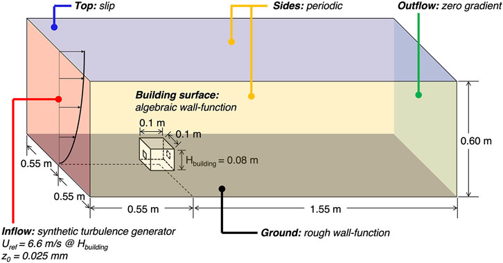
FIGURE 1. Computational domain and boundary conditions.

The computational grids for each wind direction are generated with the CharLES’ mesh generator following guidelines for meshing such as the number of cells on the edge of openings and the number of transition layers between the refinement levels (Franke, 2007). The computational grids consist of approximately 3.2 million Voronoi cells for each simulation with the smallest cell size of 1.5 mm around the building geometry. The cell size gradually increases toward the external boundary, with the biggest cell size 16 mm. A grid sensitivity study, presented in the Part I paper, showed that the flow solution and ventilation measures of interest did not change significantly when further refining the grid.

2.1.3 Inflow and Boundary Conditions

This section briefly summarizes the inflow and boundary conditions, which are identical to those used for the simulations in Part I of this study (Hwang and Gorlé, 2022). For the inflow condition, we combine a divergence-free of a digital filter method (Xie and Castro, 2008; Kim et al., 2013) with a gradient-based optimization technique to obtain the desired turbulence characteristics at the building location (Lamberti et al., 2018). The target profiles for the mean velocity, turbulence intensity and length scales are shown in Figure 2, together with the actual profiles obtained at the building location in the LES. The mean velocity profile corresponds to a logarithmic wind profile:

$U\left(z\right)=\frac{u_{\ast }}{\kappa }\log \left(\frac{z+z_0}{z_0}\right),(5)$

where u_* = 0.34 m/s is the friction velocity, κ = 0.41 is the von Karman constant, and z₀ = 0.025 mm is the roughness height. For the turbulent quantities, the streamwise stress component is obtained from the streamwise turbulence intensity (TI_u) reported for the reference experiment. The spanwise and vertical components are approximated using similarity relationships for the Reynolds stress profiles in a neutral atmospheric boundary layer (Stull, 2012):

$\overline{u^{\prime }{u}^{\prime }}\left(z\right)={\left(T{I}_u\left(z\right)\cdot U\left(z\right)\right)}^2,\overline{v^{\prime }{v}^{\prime }}\left(z\right)=\overline{w^{\prime }{w}^{\prime }}\left(z\right)=\overline{u^{\prime }{u}^{\prime }}/\sqrt{2}(6)$

For the streamwise length scale L_u, the values reported for other experiments in the same wind tunnel are used. The length scale is 0.28 m at the building height, corresponding to 56 m at full-scale. The length scales in the vertical and spanwise directions are estimated using the ratio to the streamwise component: L_v = 0.2L_u and L_w = 0.3L_u.

FIGURE 2

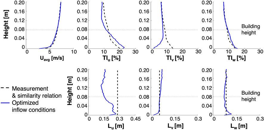
FIGURE 2. Mean velocity, turbulence intensity, and length scale profiles: target profiles (black dashed line) and profiles obtained at the building location using the optimized inflow profiles (blue solid line).

As depicted in Figure 1, wall functions are used on the building and ground surfaces: an algebraic wall model for smooth walls is specified at the building surface, while a rough wall function for a neutral ABL with a roughness length (z₀) of 0.025 mm is specified at the ground boundary. The two lateral boundaries are periodic and a slip condition is applied on the top boundary. The outlet boundary condition is set to a zero gradient condition.

2.2 Quantities of Interest for Assessing Ventilation Performance

2.2.1 Ventilation Rates

As discussed in the introduction, three different approaches to calculate the ventilation rate will be compared. First, the time-averaged ventilation rate Q_p,avg will be calculated as a function of the time-averaged pressure gradient across openings 1 and 2, |P₁ − P₂|, with $P_i=\frac{1}{T{A}_i}{\int }_0^T{\int }_{A_i}p(t)d\text{A}dt$:

$Q_{p,avg}=C_d\cdot A\cdot \sqrt{\frac{2\cdot |P_1-P_2|}{\rho }},(7)$

C_d is the still-air discharge coefficient of the openings, A is the area of one opening, and ρ is the density of air. This relation is frequently adopted in ventilation studies using both computational and experimental methods (Evola and Popov, 2006; Karava et al., 2006; Seifert et al., 2006; Karava et al., 2011), but it has two limitations. First, the discharge coefficient C_d introduces uncertainty in the equation. As in most studies, it is assumed to be a constant of 0.61, which corresponds to the value of the still-air discharge coefficient of a simple rectangular opening (Etheridge, 2011). The constant discharge coefficient is used to estimate the ventilation flow rates with Eq. 7 in Section 3.2.1. In reality, the coefficient is affected by installation effects, which are a result of multiple factors, including the wind direction (Karava et al., 2004). Second, the relation can only estimate the time-averaged flow rate and it does cannot account for the contribution of turbulent fluctuations to the air exchange process.

The second approach removes the parametric uncertainty due to C_d by estimating the time-averaged airflow rate from integration of the time-averaged normal velocity across the ventilation openings:

$Q_{u,avg}=\frac{1}{2}\left(\underset{A_1}{\int }|\mathbf{U}\cdot {\mathbf{n}}_1|d\text{A}+\underset{A_2}{\int }|\mathbf{U}\cdot {\mathbf{n}}_2|d\text{A}\right),(8)$

where $\mathbf{U}=\frac{1}{T}{\int }_0^{T}u(t)dt$ is the time-averaged velocity, n and dA are the area normal vector and the infinitesimal area of the opening. The use of the time-averaged velocity at the openings filters out any turbulent fluctuations; hence, this relationship will still be inaccurate when turbulent fluctuations have an important contribution to the air exchange.

To overcome the limitation related to time-averaging the velocity field through the openings, the third approach directly computes the instantaneous ventilation rate by using the instantaneous velocity field (u(t)):

$Q_{u,ins}\left(t\right)=\frac{1}{2}\left(\underset{A_1}{\int }|\mathbf{u}\left(t\right)\cdot {\mathbf{n}}_1|d\text{A}+\underset{A_2}{\int }|\mathbf{u}\left(t\right)\cdot {\mathbf{n}}_2|d\text{A}\right).(9)$

Then, the statistics of the ventilation rate, i.e., the mean and standard deviation, can be estimated from the time series. When the flow direction is consistent at the ventilation openings, Q_u,avg is equal to the time-average of Q_u,ins(t), which will be denoted as Q_u,ins hereafter. However, when the flow direction is variable and turbulent fluctuation plays a significant role in the ventilation process, Q_u,ins can be significantly different from Q_u,avg. The non-negligible difference between the two has been reported for single-sided ventilation (Jiang and Chen, 2001); the current study further investigates the difference in cross ventilation configurations for which turbulent air exchange plays an important role.

2.2.2 Discharge Coefficient

As discussed in Section 2.2.1, the discharge coefficient C_d adds uncertainty in the prediction of the ventilation rate using Eq. 7. The coefficient is influenced by several factors, including the opening size and shape, and the wind speed and direction (Karava et al., 2004). Previous studies have quantified the effect of the opening configuration (Kato, 2004), the opening size (Vickery and Karakatsanis, 1987; Kato, 2004), and the opening Reynolds number (Vickery and Karakatsanis, 1987; Carey and Etheridge, 1999) on C_d for a single opening under an idealized environment. However, when considering natural ventilation flow in a real building, additional installation effects, e.g. due to variations in the wind direction, can play an important role (Etheridge, 2011). These installation effects have not been accurately quantified. For example, different studies have observed different impacts of the wind direction on C_d; these differences have been attributed to differences in the size and position of a ventilation opening (Yi et al., 2019). Our LES-based analysis of the ventilation rates calculated using the three approaches introduced in Section 2.2.1 supports assessing C_d in ventilation scenarios with different opening size, opening position, and wind direction. In each case, we estimate the discharge coefficient by equating Q_u,ins with Q_p,avg,

$Q_{u,ins}=Q_{p,avg}=C_d\cdot A\sqrt{\frac{2|P_1-P_2|}{\rho }}\to C_d=\frac{Q_{u,ins}}{A\sqrt{2|P_1-P_2|/\rho }}.(10)$

When using this relationship, C_d represents a cumulative or total discharge coefficient for a cross-ventilated configuration that accounts for the installation effects. The evaluation of C_d will only be performed for the ventilation configurations with 0° and 45° wind directions, since ΔP will be approximately 0 for the 90° case due to symmetry of the building geometry.

2.2.3 Age of Air

The local age of air represents the time that a parcel of air at a certain location has resided in the indoor space. Unlike the ventilation rate, which is a space-averaged quantity, the age of air is a local quantity that can serve as a measure of the indoor air quality at a specific location. The age of air at locations x in the building is calculated using the step-down method, which consists of two steps: 1) initializing a tracer with a concentration C₀ in the indoor space and 2) recording the decay of concentration over time until it reaches the outdoor level (0 in the simulations). The age of air is then equivalent to the area under the concentration decay curve:

$\tau \left(x\right)={\int }_0^{\infty }\frac{\tilde{C}\left(x,t\right)}{C_0}dt,(11)$

where $\tilde{C}(x,t)$ is the tracer concentration at a point x at time t. The age of air calculation is performed after the initial burn-in period when a quasi steady-state solution for the flow-field has been obtained. The age of air is a good indicator for local ventilation status: τ is zero near the inlet because the air flushes out quickly, while the value is higher than average in poorly ventilated locations.

2.2.4 Ventilation Efficiency

The ventilation efficiency is a non-dimensional metric that quantifies how effectively ventilation occurs within an indoor space given a specific flow rate. Among different available definitions for the efficiency, we use the ratio of the hypothetical minimum of the average age of air, which is half the nominal time τ_n = V/Q_u,ins, to the actual spatial average of the age of air ⟨τ⟩:

$ϵ=\frac{{\tau }_n}{2⟨\tau ⟩}.(12)$

Using this definition, the ventilation efficiency is an indicator of the overall ventilation status of a space as a single non-dimensional number ranging from 0 to 1. Thus, the efficiency provides a measure for comparing different ventilation solutions in terms of the uniformity of the ‘freshness’ of the air for a given ventilation flow rate.

2.3 Ventilation Configurations of Interest

Using the computational setup presented in Section 2.1, we simulate various ventilation configurations in terms of opening size, opening position, and wind direction. Figure 3 presents the 14 cross ventilation configurations considered, each having two openings on opposite walls. In addition, the closed building, without openings, is modeled at two different wind directions to examine changes in the flow field around the building due to the presence of the openings. Of the cross-ventilation configurations, 12 cases consider a wall porosity (A_opening/A_wall) of 5% at 3 wind directions (0°, 45° and 90°), for 4 opening locations. The opening locations are: 1) both openings at the top, 2) both in the middle of facades, 3) both at bottom, and 4) the inlet at the bottom and the outlet at the top. The 2 remaining cross-ventilation cases investigate the effect of the opening size, considering a wall porosity of 10 and 20%, with a fixed wind direction of 0° and both openings in the middle of the facades. The height of openings is fixed to 18 mm for all cases; their width is 11.5, 23, and 46 mm, corresponding to the wall porosity of 5, 10 and 20%, respectively. Comparison of the ventilation measures for these different ventilation configurations will enable us to identify the relative effectiveness of each configuration.

FIGURE 3

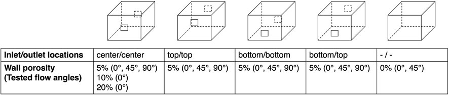
FIGURE 3. Ventilation configurations considered in the current study.

3 Results

In this section, we analyze the effect of the opening size, the opening position, and the wind direction on the ventilation flow. The results are presented in terms of velocity fields on vertical and horizontal planes through the house, as well as in terms of quantitative ventilation measures, including ventilation rates, age of air, and ventilation efficiency.

3.1 Influence of Ventilation Configuration on Flow Field

3.1.1 Effect of Opening Size

Figure 4 displays the velocity magnitude with contours and the direction with quiver plots on both vertical and horizontal planes through the center of the building geometry. The results in each column correspond to cases with different wall porosity, visualized on the top row. The wind direction is fixed to 0°, and the location of both openings is at the center. All four cases predict the typical flow features around a building such as the standing vortex in front of the windward wall, flow separation at the sharp leading edges, and re-attachment further downstream on the roof and lateral facades. The flow patterns differ the most near the openings. Compared to the sealed structure (wall porosity of 0%), the configurations with ventilation openings (wall porosity of 5, 10, and 20%) have a reduced stagnation region on the windward side near the inlet, as well as an injection of momentum into the wake on the leeward side through the outlet. The velocity patterns on the vertical plane demonstrate that both the direction and the length of the incoming and outgoing jets are quite similar for all three cases with openings. The downward direction of the inflow jet is attributed to the height of opening, where the air just upstream of the opening has a slight downward direction (Karava et al., 2011). The downward deflection of the inflow jet is slightly smaller with larger openings; this is most clearly observed on the horizontal plane. The larger openings allow more airflow directly through the building, thereby modifying the outside flow pattern and reducing the downward vertical velocity component upstream of the inlet opening.

FIGURE 4

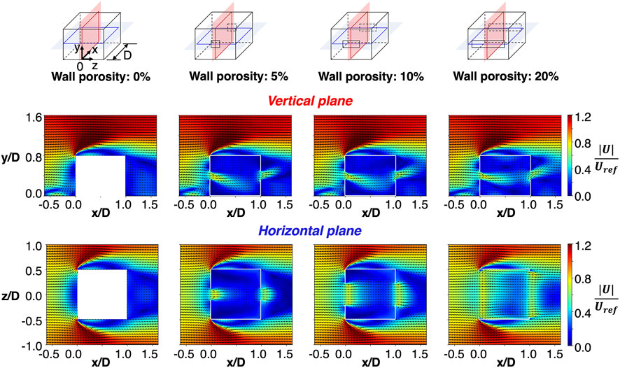
FIGURE 4. Airflow pattern in the vicinity of the building geometry for different wall porosity: 0, 5, 10 and 20% from left to right.

3.1.2 Effect of Opening Location

Figure 5 compares the flow fields on a vertical plane through the center of the building for four configurations with the inlet and the outlet at different heights. The wind direction is again fixed to 0°, and the wall porosity is 5%. Similar to the comparison of the various opening sizes in Figure 4, all simulation results reproduce the typical flow features in the vicinity of the building, regardless of the opening positions. However, the location of the openings does significantly change the directions of the inflow and outflow jets. The deflection of both jets is primarily determined by the position of the inlet. When the inlet is located near the roof, where the outdoor air moves upward, the inflow is also upwards. For all other inlet locations, the outdoor air upstream of the inlet moves downward, and the inflow is also downwards. The direction of the outflow is always opposite of the inflow. This pattern also applies to configurations not modeled here, e.g. for the inlet at the top and the outlet at the bottom, the inflow is upward and the outflow is downward (Karava et al., 2011).

FIGURE 5

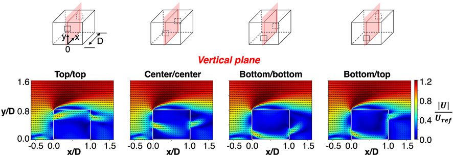
FIGURE 5. Velocity magnitude and direction on the vertical center-plane of the building in four ventilation configurations with different inlet and outlet locations.

3.1.3 Effect of Wind Direction

Figures 4, 5 demonstrated that the flow pattern is not very sensitive to the opening size, while the opening position primarily affects the vertical direction of the flow near the inlets and the outlets. For the 0° wind direction considered in these figures, the time-averaged flow field is symmetric in the horizontal. When considering different wind directions, this horizontal flow pattern changes significantly, while the vertical direction of the inflow jets is still determined by the opening position. Figure 6 visualizes the changes in the horizontal velocity by presenting the velocity field for the 0°, 45° and 90° cases on the horizontal center-plane. The wall porosity is fixed to 5% and both openings are at the center location. The results demonstrate the significant impact of the wind direction on the flow pattern, both inside and outside the building.

FIGURE 6

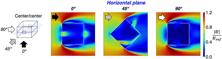
FIGURE 6. Velocity magnitude and direction on horizontal planes across openings in the center/center configurations.

The external flow pattern is very similar for the 0° and 90° wind direction, since the only difference is the location of the openings. One noteworthy difference between both cases is that the 90° case exhibits a slight decrease of the velocity magnitude in the separation region on the side of the building, just upstream of the opening. This decrease is a result of the air exchange between the outdoor separation bubble and the indoor environment. For the 45° case the differences are much more pronounced. First, the stagnation region for the 45° case is highly localized at the upstream corner of the building, while a wider stagnation region is formed for the 0° and 90° cases. Second, once the flow separates at the two corners for the 45° case, it does not reattach to the lateral walls as in the 0° and 90° cases, and a very wide wake region is formed downstream.

Considering the indoor airflow pattern, each of the three simulations shows very a different ventilation pattern. When the window opening is perpendicular to the free stream flow (0°), both the inflow and outflow jets are parallel to the free stream wind because of symmetry. When the building is rotated by 45° and the openings are at an oblique angle to the external wind, the inflow remains parallel to the wind, but the outflow is significantly deflected, with a direction that is almost perpendicular to the upstream wind direction. This deflection is a result of both the indoor flow pattern and the reduced pressure and velocity in the wake region. The 90° wind does not produce strong incoming and or outgoing flow because both the inlet and the outlet opening are parallel to the free stream wind. The lack of noticeable mean flow at the openings results in low mean velocities in the indoor environment compared to the other two cases. This does not mean that the space is not ventilated; rather, it indicates that the indoor-outdoor air exchange is primarily driven by turbulent fluctuations as in single-sided ventilation flow. To provide further insight into the importance of turbulent air exchange, Section 3.2.1 presents a quantitative comparison of the ventilation rates.

3.2 Influence of Configuration on Ventilation Measures

3.2.1 Time-Averaged and Instantaneous Ventilation Rates

The influence of opening size, opening position, and wind direction is analyzed using three different estimates of the ventilation flow rates: based on the time-averaged pressure (Q_p,avg), the time-averaged velocity (Q_u,avg), and the instantaneous velocity (Q_u,ins). Considering the opening size, the ventilation rates increase linearly with the opening size, such that the normalized ventilation rates, defined as Q/(A ⋅ U_ref), remain approximately constant for the different cases. Given this observation, the following discussion focuses on the effect of the wind direction and opening position on the normalized ventilation rate.

Figure 7 presents the estimated ventilation rates for the ventilation layout with the 5% wall porosity and both openings in the center under the different wind directions. The three rows correspond to the three wind directions of 0°, 45° and 90°. The plots present the time series and corresponding distribution of the normalized Q_u,ins(t) and it includes the average values obtained from Q_p,avg and Q_u,avg for comparison. The red dashed line in the 0° case (top row) is the PIV measurement from the reference wind-tunnel experiment (Karava et al., 2011). For the 0° wind direction, all three LES predictions compare well to each other and to the measurement. In the 45° case, the pressure-based non-dimensional ventilation rate starts to deviate from the velocity-based values by 10%. This discrepancy can be attributed to the fact that the discharge coefficient C_d varies as a function of the wind direction. For the wind direction of 90°, Q_p,avg is expected to be 0, since the symmetry in the flow results in the average pressure difference between the openings being 0. The fact that the calculated rate is not exactly 0 can be attributed to statistical convergence errors. The mean velocity field is also symmetrical, but there is a very small bi-directional mean flow through each opening, such that Q_u,avg predicts a very small ventilation rate. Finally, Q_u,ins, which is the only measure that can account for turbulent air exchange, predicts a ventilation rate that is more than twice the value of Q_u,avg.

FIGURE 7

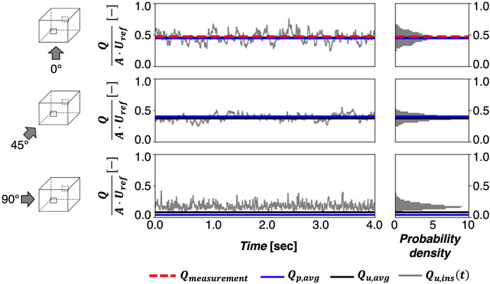
FIGURE 7. LES predictions of ventilation rate using velocity (left) and pressure (right) for the 0°(top), 45°(middle), and 90°(bottom) wind directions.

Figure 8 summarizes the predictions of the normalized ventilation rates for all wind directions and configurations. The three columns correspond to the three wind directions and the four rows correspond to four ventilation configurations with different positions for the inlet and outlet. For each case, the blue, black, and Gy bars indicate the ventilation rates computed with the time-averaged pressure, the time-averaged velocity, and the instantaneous velocity fields. The results confirm that the observations from Figure 7 hold across the different configurations. First, for the 0° wind direction, the ventilation rates calculated using the different methods agree quite well. For the configurations that have openings closer to the roof or the floor, a discrepancy of 10% occurs between the pressure-based and velocity-based estimates. These differences can be attributed to the fact that changes in the flow directions just upstream and downstream of the openings will affect the value of C_d. Second, for the 45° wind direction, the discrepancies between the pressure-based and velocity-based estimates are on the order of 10% for all configurations. Again, the change in the wind direction affects the flow directions upstream and downstream of the openings, which in turn affects C_d. This finding is consistent with previous research (Karava et al., 2004). Third, the 90° case shows the largest difference between the three predictions. The pressure-based predictions for configurations where the openings are positioned at the same height are negligibly small due to the symmetry in the flow. When the openings are located at different heights, there is a small pressure difference that predicts a slightly higher ventilation rate. The predictions based on the average velocity also predict small ventilation rates, due to a small bi-directional mean flow through each opening. In all configurations, the values based on the instantaneous velocity predict ventilation rates that are up to two times higher. This confirms that the averaging process used when calculating Q_p,avg and Q_u,avg filters out the velocity fluctuations that dominate ventilation flow for the 90° wind direction.

FIGURE 8

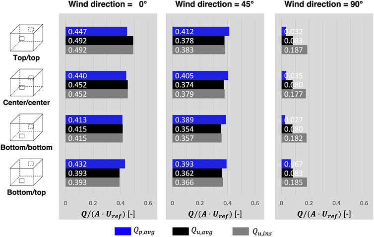
FIGURE 8. Summary of non-dimensional ventilation rate under four different ventilation configurations and three different wind directions.

Comparing the values of Q_ins across all wind directions and all configurations, it is observed that the wind direction has a more important effect than the location of the openings. The 0° cases consistently show the highest ventilation rate. The ventilation rates are 7–22% lower for the 45° case, and 53–62% lower for the 90° case. Across the different opening locations, the configuration with both openings at the top has the highest ventilation rate. This higher ventilation rate occurs because the inlet directly encounters higher wind speeds at this higher height and because the pressure at the outlet is lower. The maximum decrease compared to this configuration varies from 5% for the 45° and 90° wind directions to 20% for the 0° wind direction.

3.2.2 Discharge Coefficient

As presented in Section 3.2.1, the ventilation rate estimated using the pressure difference between the openings (Eq. 7) can be inaccurate when using a constant discharge coefficient (C_d = 0.61). This discrepancy was indeed observed in Sec. 3.2.1. In this section, we compute the value for C_d that results in Q_p,avg being equal to Q_u,ins for 10 different cross-ventilated configurations with different wall porosity, opening position, and wind direction (see Figure 3). The configurations with a wind direction of 90° are not included, considering that the mean pressure difference is zero due to the symmetry in the flow field. In Figure 9, the resulting C_d is plotted against the corresponding opening Reynolds number (Re_o = U_opening ⋅ d_h/ν), where U_opening = Q_u,ins/A is the velocity at the opening, d_h is the hydraulic diameter of the opening, and ν is the kinematic viscosity of air.

FIGURE 9

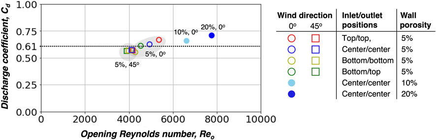
FIGURE 9. Total discharge coefficient vs. opening Reynolds number.

The estimated C_d values vary from 0.53 to 0.71. Considering first the same wall porosity of 5%, the discrepancy in C_d can be explained as an installation effect, because the size and the shape of the openings are identical but their position varies. As a result, the C_d values can largely be categorized according to the wind direction. For the 45° cases, C_d ≈ 0.57, regardless of the opening position. These cases also have very similar flow rates, and hence similar values of Re_o. For the 0° cases, there is a more significant variation in both C_d and Re_o. In general, C_d is larger than for the 45° cases, and the values are linearly correlated with Re_o. We note that this result does not imply that the C_d value for a specific opening at a specific location is a function of Re_o. To investigate such a relationship, simulations with identical configurations but different incoming wind speeds should be compared. Finally, considering the effect of the wall porosity, the results indicate that C_d increases with wall porosity. Similarly, Re_o increases linearly with the porosity, since larger openings have a larger hydraulic diameter. In summary, the results demonstrate that C_d is a function of multiple parameters, including the wind direction, the opening location, and the opening size. This finding is consistent with previous studies (Vickery and Karakatsanis, 1987; Carey and Etheridge, 1999; Karava et al., 2004; Kato, 2004; Etheridge, 2011; Yi et al., 2019).

3.2.3 Age of Air

The ventilation rate gives information on the overall air indoor/outdoor air exchange, but it does not reveal whether a space is uniformly ventilated. The local age of air, computed at 94,000 uniformly distributed points, provides this additional insight. Assuming that the local age of air is inversely correlated to the velocity fields visualized in Section 3.1, it can be expected that the spatial distribution of the age of air is more sensitive to the wind direction than to the size or the position of the openings. Hence, Figure 10 first visualizes the local age of air on the horizontal center-plane for the 0°, 45°, and 90° wind directions with the opening locations fixed at the center.

FIGURE 10

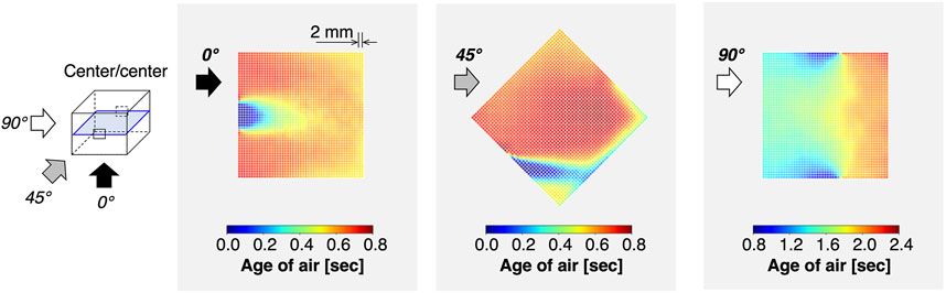
FIGURE 10. Distribution of mean age of air on the horizontal mid-plane of the building for different wind directions. Color scaling for the 90° case reflects the higher age of air compared to the 0° and 45° cases.

For the 0° and 45° degree wind directions, the age of air values indeed show an inverse correlation with the corresponding velocity magnitudes shown in Figure 6: the higher the velocity magnitude at a point, the lower the mean age at that point. This correlation occurs because of a well established mean flow pattern, where the air near the inlet has the highest velocity and the lowest age. For the 90° case, this mean flow pattern is not observed. With the window openings being parallel to the mean wind direction, ventilation occurs primarily through turbulent air exchange. The resulting age of air is significantly higher, with the minimum values near the openings on the order of the maximum values observed in the 0° and 45° cases. The resulting spatial distribution of the age of air is also non-uniform, with the indoor area downstream of the window opening less well ventilated than the upstream region.

Figure 11 visualizes the effects of the wind direction (A), the opening position (B), and the wall porosity (C) on the frequency distributions of the age of air collected from all uniformly distributed points in the indoor space. In each plot, one parameter is varied, while the other two are fixed. Regarding the effect of the wind direction, Figure 11A confirms the observations from Figure 10. First, the age of air is two to three times higher for the 90° case than for the 0° and 45°, due to the absence of significant mean flow. Second, the non-uniform ventilation of the indoor space in the 90° case is reflected in the bi-modal shape of the frequency distribution. An additional observation is that the distributions for the 0° and 45° degree cases have very similar mean values (0.612 vs. 0.637), but their shapes indicate that the 0° case provides a better overall ventilation pattern.

FIGURE 11

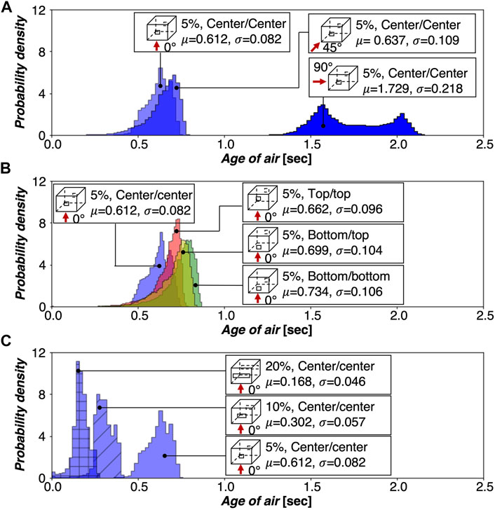
FIGURE 11. Distribution of age of air.

Figure 11B visualizes the impact of the different inlet and outlet positions, which is less pronounced than the influence of the wind direction. The distributions are quite similar, with maximum differences of 20% in the mean values and 30% in the standard deviations. The differences are related to the changing directions of the inflow shown in Figure 5. The spatial mean of the age is lowest for the center/center configuration, when the airflow entering through the inlet does not interact with the roof or the flow. The mean age increases when the inlet is at the top or the bottom and the airflow entering through the inlet does interact with the roof or the floor. The mean age of air is 8% higher for the top/top configuration than for the center/center configuration, even though the ventilation flow rate is 9% higher. For the bottom/bottom and bottom/top configurations, the mean age is 14 and 20% higher, respectively.

Finally, Figure 11C presents the effect of the wall porosity. As expected, larger openings result in a smaller mean value and a smaller standard deviation of the spatial distribution of the age, since the larger openings allow more airflow through a larger portion of the indoor space. This decreasing trend of mean age with respect to the opening size agrees with the increasing trend in ventilation rate.

Table 1 summarizes the mean and standard deviation of the spatial distribution of the age of air for the 12 ventilation scenarios, where the three columns correspond to different wind directions and the four rows correspond to different opening locations. All configurations shown have a wall porosity of 5%. The reported statistics confirm the observations based on the few sample results in Figure 11: the mean age increases non-linearly as the wind direction changes from 0° to 90° for all ventilation configurations, and the influence of the opening location is smaller than the influence of the wind direction. Comparison to the ventilation rates reported in Figure 8 indicates that the spatial average of the age is generally negatively correlated with the ventilation rate, although exceptions occur when the flow pattern changes due to the location of the inlet.

TABLE 1

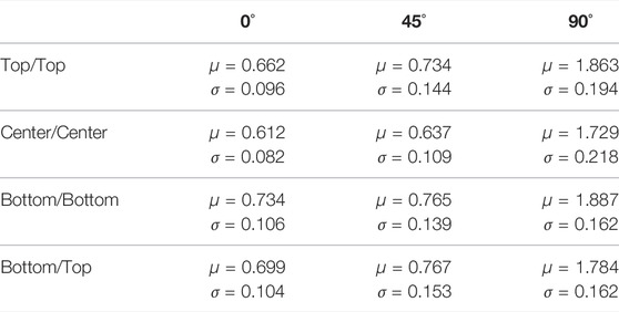
TABLE 1. Summary of age of air statistics for ventilation configurations with a wall porosity of 5%.

3.2.4 Ventilation Efficiency

The ventilation efficiency, which is the ratio of the ventilation rate in terms of the nominal time to twice the spatial average of the age of air, is a commonly used non-dimensional metric that represents how effectively ventilation occurs in a space. Table 2 summarizes the ventilation efficiency for the 12 ventilation configurations for which the age of air statistics were presented in Table 1. All configurations have an efficiency greater than 0.426, with the highest value of 0.606 for the configuration with the openings in the center and a wind direction of 45°. When both the inlet and the outlet are at the same height (top/top, center/center and bottom/bottom), the wind direction of 45° is the most efficient, followed by the 0° and 90° wind directions. For the configuration with the inlet at the bottom and the outlet at the top, the 0° and 45° wind directions have similar efficiencies. The 90° wind direction is the least efficient in all cases. Considering the opening locations, the configuration with the openings at the center is most efficient, independent of the wind direction. The central location of the inflow results in more efficient mixing throughout the indoor environment. When both openings are at the top or the bottom, the opposite side of the room is less efficiently ventilated. By placing one opening at the bottom and one a the top, the efficiency can be somewhat increased, because the air is forced to flow vertically between the inlet and the outlet opening.

TABLE 2

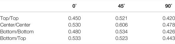
TABLE 2. Summary of ventilation efficiency.

To conclude, we note that the efficiency as defined in the current study does not directly indicate freshness of a space; instead, it represents how effectively ventilation occurs within the space given the amount of fresh air coming into the space. As a result, a high ventilation efficiency does not necessarily imply a well-ventilated space. For example, the efficiency for a specific configuration is at most 25% lower for the 90° wind direction than for the 0° wind direction, despite the much higher age of air in the 90° cases (see Figure 11). To ensure that sufficient fresh air is efficiently supplied to an indoor space, the ventilation flow rate and the age of air should be considered independently.

4 Conclusion and Future Work

LES simulations of an isolated building with wind-driven cross ventilation were performed to investigate the effect of the opening size, opening location, and wind direction on the ventilation flow. The effects are quantified using different ventilation measures, including time-averaged and instantaneous ventilation flow rates, the age of air and the ventilation efficiency.

Considering the ventilation rate, the simulation results indicate: 1) linear scaling of the ventilation rate with the opening area, 2) a pronounced effect of the wind direction, with a decrease in the ventilation rate of up to 62% when the wind direction changes from 0° to 90°, and 3) a smaller effect of the opening location, with differences in the ventilation rate of up to 20%. Considering a fixed wall porosity of 5%, the ventilation rate was found to be highest for the 0° wind direction with both openings at the top. As the inlet opening moves closer to the ground, and as the wind direction increases to 90°, the ventilation rate decreases. Comparison of the ventilation rates calculated using the time-averaged pressure difference and the time-averaged velocity show differences of around 10% for the 0° and 45° wind directions. These differences are due to installation effects that affect the value of the discharge coefficient. Since these wind directions have a well-defined mean flow through the upstream opening, the differences between ventilation rates calculated using the time-averaged and instantaneous velocity are negligible. In contrast, for the 90° wind direction, the mean flow velocity is negligible, and the ventilation process is driven by turbulent air exchange at both lateral openings. When turbulent fluctuations are the primary ventilation mechanism, an accurate calculation of the ventilation rate requires knowledge of the instantaneous velocity field.

The spatial average of the age of air is generally found to be negatively correlated with the overall flow rate, although exceptions are found to occur when the location of the openings changes the flow pattern and corresponding age distribution. For example, considering the configurations with 5% porosity for the 0° and 45° wind direction, the configuration with both openings at the top has the highest flow rates, but it also has a slightly higher mean and standard deviation for the age of air than the case with both openings at the center. This result indicates the added value of information on the spatial distribution of the age of air when evaluating different design options.

Lastly, the ventilation efficiency was found to be highest for the configuration with both openings in the center, and the wind direction for 45°. We note that the efficiency should be interpreted with care, since it only provides a metric of how efficiently the space is ventilated given the specific ventilation flow rate. Hence, it does not reflect the overall freshness of air in the space.

The results of this study indicate the significant potential of LES towards assessing wind-driven natural ventilation performance. The simulation results provide accurate information on the overall ventilation flow rate, while also providing insight into the spatial distribution of the age of air. The model used in the current study represented a reference wind tunnel experiment of an idealized configuration, but it can easily be expanded to consider more realistic building configurations in urban environments. Future parametric studies of more realistic cases could have practical implications for the design of buildings with natural ventilation, providing a basis for developing reduced order representations for ventilation rates that can be leveraged in building energy models.

Data Availability Statement

The raw data supporting the conclusions of this article will be made available by the authors, without undue reservation.

Author Contributions

YH performed simulations and formal analysis of results, and wrote the original draft of the manuscript. CG created the research plan, supervised the project, and revised the manuscript.

Funding

This research was funded by a seed grant from the Stanford Woods Institute Environmental Venture Projects program and supported by the Stanford Center at the Incheon Global Campus (SCIGC) funded by the Ministry of Trade, Industry, and Energy of the Republic of Korea and managed by the Incheon Free Economic Zone Authority. The simulations were performed using the Extreme Science and Engineering Discovery Environment (XSEDE), which is supported by National Science Foundation grant number CI-1548562.

Conflict of Interest

The authors declare that the research was conducted in the absence of any commercial or financial relationships that could be construed as a potential conflict of interest.

Publisher’s Note

All claims expressed in this article are solely those of the authors and do not necessarily represent those of their affiliated organizations, or those of the publisher, the editors and the reviewers. Any product that may be evaluated in this article, or claim that may be made by its manufacturer, is not guaranteed or endorsed by the publisher.

References

Ambo, K., Nagaoka, H., Philips, D., Ivey, C., Brès, G., and Bose, S. (2020). “Aerodynamic Force Prediction of the Laminar to Turbulent Flow Transition Around the Front Bumper of the Vehicle Using Dynamic-Slip Wall Model LES,” in AIAA Scitech 2020 Forum: Orlando, FL (Reston, VA: American Institute of Aeronautics and Astronautics). doi:10.2514/6.2020-0036

CrossRef Full Text | Google Scholar

Artmann, N., Manz, H., and Heiselberg, P. (2007). Climatic Potential for Passive Cooling of Buildings by Night-Time Ventilation in Europe. Appl. energy 84, 187–201. doi:10.1016/j.apenergy.2006.05.004

CrossRef Full Text | Google Scholar

Asfour, O. S., and Gadi, M. B. (2007). A Comparison between Cfd and Network Models for Predicting Wind-Driven Ventilation in Buildings. Build. Environ. 42, 4079–4085. doi:10.1016/j.buildenv.2006.11.021

CrossRef Full Text | Google Scholar

Bhagat, R. K., Davies Wykes, M. S., Dalziel, S. B., and Linden, P. F. (2020). Effects of Ventilation on the Indoor Spread of COVID-19. J. Fluid Mech. 903, F1. doi:10.1017/jfm.2020.720

PubMed Abstract | CrossRef Full Text | Google Scholar

Caciolo, M., Stabat, P., and Marchio, D. (2012). Numerical simulation of single-sided ventilation using rans and les and comparison with full-scale experiments. Build. Environ. 50, 202–213. doi:10.1016/j.buildenv.2011.10.017

CrossRef Full Text | Google Scholar

Carey, P. S., and Etheridge, D. W. (1999). Direct Wind Tunnel Modelling of Natural Ventilation for Design Purposes. Build. Serv. Eng. Res. Technol. 20, 131–142. doi:10.1177/014362449902000305

CrossRef Full Text | Google Scholar

[Dataset] Cascade Technologies, Inc. (2022). CharLES. Available at: https://www.cascadetechnologies.com.

Google Scholar

Etheridge, D. (2011). Natural Ventilation of Buildings: Theory, Measurement and Design. Chichester, UK: John Wiley & Sons.

Google Scholar

Evola, G., and Popov, V. (2006). Computational Analysis of Wind Driven Natural Ventilation in Buildings. Energy Build. 38, 491–501. doi:10.1016/j.enbuild.2005.08.008

CrossRef Full Text | Google Scholar

Franke, J. (2007). Best Practice Guideline for the CFD Simulation of Flows in the Urban Environment. Brussels, Belgium: Meteorological Inst.

Google Scholar

Ham, F., and Iaccarino, G. (2004). Energy Conservation in Collocated Discretization Schemes on Unstructured Meshes. Stanford, CA: Center for Turbulence Research, NASA Ames/Stanford University Stanford, 3–14.

Google Scholar

Hu, C.-H., Ohba, M., and Yoshie, R. (2008). Cfd modelling of unsteady cross ventilation flows using les. J. Wind Eng. Industrial Aerodynamics 96, 1692–1706. doi:10.1016/j.jweia.2008.02.031

CrossRef Full Text | Google Scholar

Hwang, Y., and Gorlé, C. (2022). Large Eddy Simulations of Wind-Driven Cross Ventilation, Part 1: Validation and Sensitivity Study. Front. Built Environ. 8. doi:10.3389/fbuil.2022.911005

CrossRef Full Text | Google Scholar

Jiang, Y., Alexander, D., Jenkins, H., Arthur, R., and Chen, Q. (2003). Natural Ventilation in Buildings: Measurement in a Wind Tunnel and Numerical Simulation with Large-Eddy Simulation. J. Wind Eng. Industrial Aerodynamics 91, 331–353. doi:10.1016/s0167-6105(02)00380-x

CrossRef Full Text | Google Scholar

Jiang, Y., and Chen, Q. (2003). Buoyancy-driven Single-Sided Natural Ventilation in Buildings with Large Openings. Int. J. Heat Mass Transf. 46, 973–988. doi:10.1016/s0017-9310(02)00373-3

CrossRef Full Text | Google Scholar

Jiang, Y., and Chen, Q. (2001). Study of Natural Ventilation in Buildings by Large Eddy Simulation. J. Wind Eng. industrial aerodynamics 89, 1155–1178. doi:10.1016/s0167-6105(01)00106-4

CrossRef Full Text | Google Scholar

Karava, P., Stathopoulos, T., and Athienitis, A. K. (2011). Airflow Assessment in Cross-Ventilated Buildings with Operable Façade Elements. Build. Environ. 46, 266–279. doi:10.1016/j.buildenv.2010.07.022

CrossRef Full Text | Google Scholar

Karava, P., Stathopoulos, T., and Athienitis, A. K. (2006). Impact of Internal Pressure Coefficients on Wind-Driven Ventilation Analysis. Int. J. Vent. 5, 53–66. doi:10.1080/14733315.2006.11683724

CrossRef Full Text | Google Scholar

Karava, P., Stathopoulos, T., and Athienitis, A. K. (2004). Wind Driven Flow through Openings - A Review of Discharge Coefficients. Int. J. Vent. 3, 255–266. doi:10.1080/14733315.2004.11683920

CrossRef Full Text | Google Scholar

Kato, S. (2004). Flow Network Model Based on Power Balance as Applied to Cross-Ventilation. Int. J. Vent. 2, 395–408. doi:10.1080/14733315.2004.11683681

CrossRef Full Text | Google Scholar

Kim, Y., Castro, I. P., and Xie, Z.-T. (2013). Divergence-free Turbulence Inflow Conditions for Large-Eddy Simulations with Incompressible Flow Solvers. Comput. Fluids 84, 56–68. doi:10.1016/j.compfluid.2013.06.001

CrossRef Full Text | Google Scholar

Kwon, K.-S., Lee, I.-B., Han, H.-T., Shin, C.-Y., Hwang, H.-S., Hong, S.-W., et al. (2011). Analysing Ventilation Efficiency in a Test Chamber Using Age-Of-Air Concept and Cfd Technology. Biosyst. Eng. 110, 421–433. doi:10.1016/j.biosystemseng.2011.08.013

CrossRef Full Text | Google Scholar

Lamberti, G., García-Sánchez, C., Sousa, J., and Gorlé, C. (2018). Optimizing Turbulent Inflow Conditions for Large-Eddy Simulations of the Atmospheric Boundary Layer. J. Wind Eng. Industrial Aerodynamics 177, 32–44. doi:10.1016/j.jweia.2018.04.004

CrossRef Full Text | Google Scholar

Murakami, S., and Kato, S. (1992). “New Scales for Ventilation Efficiency and Their Application Based on Numerical Simulation of Room Airflow,” in Proceedings of International Symposium on Room Air Convection and Ventilation Effectiveness (Tokyo: University of Tokyo), 22–38.

Google Scholar

Panagopoulos, I. K., Karayannis, A. N., Kassomenos, P., and Aravossis, K. (2011). A CFD Simulation Study of VOC and Formaldehyde Indoor Air Pollution Dispersion in an Apartment as Part of an Indoor Pollution Management Plan. Aerosol Air Qual. Res. 11, 758–762. doi:10.4209/aaqr.2010.11.0092

CrossRef Full Text | Google Scholar

Prajongsan, P., and Sharples, S. (2012). Enhancing Natural Ventilation, Thermal Comfort and Energy Savings in High-Rise Residential Buildings in Bangkok through the Use of Ventilation Shafts. Build. Environ. 50, 104–113. doi:10.1016/j.buildenv.2011.10.020

CrossRef Full Text | Google Scholar

Ramponi, R., Angelotti, A., and Blocken, B. (2014). Energy Saving Potential of Night Ventilation: Sensitivity to Pressure Coefficients for Different European Climates. Appl. Energy 123, 185–195. doi:10.1016/j.apenergy.2014.02.041

CrossRef Full Text | Google Scholar

Sandberg, M., and Sjöberg, M. (1983). The Use of Moments for Assessing Air Quality in Ventilated Rooms. Build. Environ. 18, 181–197. doi:10.1016/0360-1323(83)90026-4

CrossRef Full Text | Google Scholar

Sandberg, M. (1981). What Is Ventilation Efficiency? Build. Environ. 16, 123–135. doi:10.1016/0360-1323(81)90028-7

CrossRef Full Text | Google Scholar

Seifert, J., Li, Y., Axley, J., and Rösler, M. (2006). Calculation of Wind-Driven Cross Ventilation in Buildings with Large Openings. J. Wind Eng. Industrial Aerodynamics 94, 925–947. doi:10.1016/j.jweia.2006.04.002

CrossRef Full Text | Google Scholar

Shirzadi, M., Mirzaei, P. A., and Naghashzadegan, M. (2018). Development of an Adaptive Discharge Coefficient to Improve the Accuracy of Cross-Ventilation Airflow Calculation in Building Energy Simulation Tools. Build. Environ. 127, 277–290. doi:10.1016/j.buildenv.2017.10.019

CrossRef Full Text | Google Scholar

Stavrakakis, G. M., Koukou, M. K., Vrachopoulos, M. G., and Markatos, N. C. (2008). Natural Cross-Ventilation in Buildings: Building-Scale Experiments, Numerical Simulation and Thermal Comfort Evaluation. Energy Build. 40, 1666–1681. doi:10.1016/j.enbuild.2008.02.022

CrossRef Full Text | Google Scholar

Stull, R. B. (2012). An Introduction to Boundary Layer Meteorology, Vol. 13. Dordrecht, Netherlands: Springer Science & Business Media.

Google Scholar

Sun, X., Park, J., Choi, J.-I., and Rhee, G. H. (2017). Uncertainty Quantification of Upstream Wind Effects on Single-Sided Ventilation in a Building Using Generalized Polynomial Chaos Method. Build. Environ. 125, 153–167. doi:10.1016/j.buildenv.2017.08.037

CrossRef Full Text | Google Scholar

Urrego, J., Andrews, J. R., Yeckel, C. W., Sgarbi, R. V. E., Croda, J., Paião, D. S. G., et al. (2015). The Impact of Ventilation and Early Diagnosis on Tuberculosis Transmission in Brazilian Prisons. Am. J. Trop. Med. Hyg. 93, 739–746. doi:10.4269/ajtmh.15-0166

PubMed Abstract | CrossRef Full Text | Google Scholar

van Hooff, T., Blocken, B., and Tominaga, Y. (2017). On the accuracy of cfd simulations of cross-ventilation flows for a generic isolated building: comparison of rans, les and experiments. Build. Environ. 114, 148–165. doi:10.1016/j.buildenv.2016.12.019

CrossRef Full Text | Google Scholar

Vickery, B., and Karakatsanis, C. (1987). External Wind Pressure Distributions and Induced Internal Ventilation Flow in Low-Rise Industrial and Domestic Structures. ASHRAE Trans. 93, 2198–2213.

Google Scholar

Vreman, A. W. (2004). An Eddy-Viscosity Subgrid-Scale Model for Turbulent Shear Flow: Algebraic Theory and Applications. Phys. fluids 16, 3670–3681. doi:10.1063/1.1785131

CrossRef Full Text | Google Scholar

Weaver, A. M., Sharmin, I., Parveen, S., Crabtree-Ide, C., Luby, S. P., Mu, L., et al. (2017). Pilot Intervention Study of Household Ventilation and Fine Particulate Matter Concentrations in a Low-Income Urban Area, Dhaka, bangladesh. Am. J. Trop. Med. Hyg. 97, 615–623. doi:10.4269/ajtmh.16-0326

PubMed Abstract | CrossRef Full Text | Google Scholar

Xie, Z.-T., and Castro, I. P. (2008). Efficient Generation of Inflow Conditions for Large Eddy Simulation of Street-Scale Flows. Flow. Turbul. Combust. 81, 449–470. doi:10.1007/s10494-008-9151-5

CrossRef Full Text | Google Scholar

Xing, H., Hatton, A., and Awbi, H. B. (2001). A Study of the Air Quality in the Breathing Zone in a Room with Displacement Ventilation. Build. Environ. 36, 809–820. doi:10.1016/s0360-1323(01)00006-3

CrossRef Full Text | Google Scholar

Yi, Q., Wang, X., Zhang, G., Li, H., Janke, D., and Amon, T. (2019). Assessing Effects of Wind Speed and Wind Direction on Discharge Coefficient of Sidewall Opening in a Dairy Building Model - A Numerical Study. Comput. Electron. Agric. 162, 235–245. doi:10.1016/j.compag.2019.04.016

CrossRef Full Text | Google Scholar