Parameter identification approach to represent building thermal dynamics reducing tuning time of control system gains: A case study in a tropical climate

1 Introduction

The buildings sector accounts for around a third of final energy consumption. This energy is mostly used by heating, ventilation, and air conditioning (HVAC) systems (Wang and Chen 2019). In Panama, a hot and humid tropical climate, most electrical energy consumption is due to air conditioning systems in buildings. The residential sector is expected to increase the electrical energy used for air conditioning by at least 50% by 2050 (Secretaría Nacional de Energía, 2017).

This trend in elevated electrical energy consumption by HVAC systems has propelled the scientific community and the industry to reduce HVAC consumption without incurring costly alternatives such as retrofitting. Consequently, attention has been focused on improving the thermal performance of buildings through controller design, operational optimization, energy management, and ongoing commissioning (Wang and Chen 2019). A key element required to implement these strategies is a thermal model that characterizes the building envelope and systems used to provide cooling, heating, or ventilation (Cui et al., 2019). A thermal model is also fundamental for other uses such as demand response, peak load shifting, cooling load prediction, and energy use forecasting (Cui et al., 2019).

A control-oriented model of building dynamics should be a middle ground between a sufficiently accurate representation of heat transfer processes and a computationally efficient model resolution for optimal controller performance (Li and Jin 2014). Several authors have categorized the techniques used to formulate thermal building models. The most popular classification, adopted by many authors (Zhao and Magoulès 2012; Derakhtenjani et al., 2015; Harish and Kumar 2016; Bourdeau et al., 2019; Kathirgamanathan et al., 2021), categorizes building thermal models as white-box models, black-box models, and gray-box models.

White box models also called physical models or a forward approach, represent building thermal dynamics through physical equations, such as energy balances. Their parametric structure is derived from physical laws, and the model’s parameters, which complete the representation, are all known a priori. These can be obtained from the building’s thermal properties, construction, occupancy profiles, and climate data.

According to the degree of detail used to describe the properties and states of the building, white box models can be further classified into three approaches: computational fluid dynamics (CFD), zonal approach, and nodal approach (Foucquier et al., 2013). The CFD approach divides the system into control volumes, forming a mesh. For each control volume, Navier-Stokes’s equations are solved. The zonal approach simplifies CFD, dividing the system into control surfaces, for each of which the heat transfer equations are solved (Çengel and Cimbala 2018). Despite the level of detail these approaches provide, the fine mesh size of these models makes them too computationally demanding for control or simulation purposes. Furthermore, such a detailed description of states is not needed for building energy modeling, as the spatial variations of temperature, pressure, and CO2 are not significant in some applications.

On the other hand, the nodal approach divides the system in zones, each of them constituting a node. A node can represent building elements, such as walls or windows or a large volume of indoor air. Heat transfer equations are solved accounting for the network of nodes (Foucquier et al., 2013). The nodal approach assumes that states’ variations (such as temperature) for a volume are not significant, considering them to be uniform. Therefore, a single node can represent the whole bulk of indoor air within the room and can be described by a single temperature without incurring in significant error, which greatly reduces the mesh size. This results in a more computationally efficient model, which is why it is the most popular approach to derive building thermal models.

While the nodal approach reduces the computational demands of the model, its resolution times are still unsuitable for control purposes. The resulting high-order model is still time-consuming to solve. Moreover, the need to know beforehand the building parameters difficults the modeling procedure since this information can be difficult to obtain or unavailable. Therefore, white-box models are used to build reference models, which are supposed to represent the “real” system. Energy simulation softwares, such as Energy Plus (EP), TRNSYS, DOE, and ESP-r, employ the nodal approach to build such models. Then, during simulation, these reference models are excited to generate the training and validation data to identify another model type. In (Gray and Schmidt 2018), the authors use TRNSYS and MATLAB to model a single zone office. The building envelope, radiators, and chilled ceilings are modeled in TRNSYS, while the rest of the HVAC system is modeled in MATLAB. In (Liu et al., 2016) the authors use EP to model a multizone office building. The modeled heat sources in EP include HVAC, lighting, occupant heat gains, infiltration, equipment, and climate conditions. For both (Liu et al., 2016; Gray and Schmidt 2018), these models are simulated in the software to obtain the training and validation data to identify grey and black-box models.

The difficulty of modeling complex processes using exclusively physical principles gives way to system identification, defined by Ljung as “building mathematical models of dynamical systems based on observed data from the systems” (Ljung 1999). The system identification process starts with the excitation of the systems to be modeled and data recollection. Next, a tunable parametric model structure is chosen. Model parameters are then regressed from data using a chosen parameter estimation method. Model performance is assessed according to an established performance criterion. If the desired performance is not achieved, one of the main components of the system identification processes is adjusted, and the loop is repeated (Isermann and Münchhof 2011). Black box and grey box models use the system identification approach to obtain a suitable representation of processes.

Black-box models also referred to as the inverse approach, regress the mathematical relations that describe the system through the available input and output data without using the system’s physical knowledge. While black-box modeling techniques can be classified in several ways, in this paper, they are classified as in (Drgoňa et al., 2020): linear parametric models, nonlinear parametric models, and nonlinear non-parametric models. Parametric models are structured through a finite number of parameters. Non-parametric models, on the other hand, implicitly contain system parameters and are often presented through diagrams, characteristic curves, and tables (Tangirala 2018).

Linear parametric models include autoregressive models, such as ARX, ARMAX, ARIMAX, and state-space models. In (Paschke and Zaiczek 2018), the authors use an ARIMAX model to predict the indoor temperature in a conference room. Model inputs include heat rejected by radiators and fan coils, exterior temperature, and solar heat gains. The model is trained with measured data from sensors located in the room. When validated with data corresponding to unoccupied periods, the model has an absolute error of 0.6 K for 95% of predictions with a 4-h horizon. In (Gorni et al., 2016), the authors use domain knowledge to estimate the approximate order of an ARMAX model to predict the indoor temperature in a residential building. Model inputs include the temperature of adjacent rooms, exterior temperature, solar radiation, and heat rejected by fan coils. With a seventh order model, validation results show a maximum error of 0.5 K (Chen et al., 2016). make use of domain knowledge as well, given that heat transfer processes have a fractional nature, and use a FARX model to predict indoor temperature in a residential building. Model inputs include solar, internal, and infiltration gains, exterior temperature, and heat rejected or supplied by the air handling unit. A FARX model of order six results in an absolute error of 0.264°C, like the one obtained by a 100th order ARX model. This shows the advantage of incorporating domain knowledge into model selection. (Liu et al., 2016) model the indoor temperature of a multizone building with a state-space model of order 57, the latter determined through a cross-validation procedure. Model inputs include power consumption by the HVAC system, exterior temperature, and internal gains. The model produces an average squared error of 3%.

Multi-variable regression models are widely used to model the thermal behavior of buildings and forecast important quantities such as indoor temperature and heating power. (Bilous et al., 2018) formulate a nonlinear multivariable regression model to estimate the indoor temperature taking into account several internal and external influential factors such as heating level, outdoor air temperature and solar gains. Each influential factor is analyzed individually. For example, it is found that the change of indoor temperature due to disturbances of outdoor temperature is close to logarithmic. The accuracy of the regression model is assessed estimating the corrected determination coefficient, 0.981 and the Fisher’s criterion 1,324.3 which indicates a highly reliable regression. (Cholewa et al., 2021) develop a modeling methodology that describes the thermal behavior of a building in terms of an equivalent outdoor temperature. Three buildings are used to implement the methodology, a multifamily building (A), a health clinic (B) and a supermarket (C). It is only possible to obtain a regression model for buildings A and B due to the type of heating system available which uses a form of weather compensation for regulating supply temperature. Building C uses a traditional ON OFF control. The resulting regression models include a positive correction coefficient for equivalent outdoor temperature due to wind velocity and negative due to solar radiation. For buildings A and B the determination coefficient obtained is 0.9362 and 0.9116, respectively. This procedure is used in (Cholewa et al., 2022) to apply a an easy implementable forecast control that achieves up to 15% energy savings by means of preheating.

One of the most popular nonlinear parametric black-box models is artificial neural networks (ANN). ANN’s are used for describing all sorts of nonlinear behavior in various fields. Their adaptive nature is an advantage to model time variant phenomena found in economics, biology, politics, engineering, etc. For instance, (Anđelković and Bajatović 2020), uses an ANFIS model to forecast the natural gas consumption 1 hour ahead, from consumption, weather and calorific values data. These models establish input-output relations through a structure that emulates how the human brain works. A simple ANN architecture typically consists of one input layer, a single hidden layer, and an output layer (Amasyali and El-Gohary 2018). In (Finck et al., 2019), the authors use ANNs to predict weather conditions, HVAC system parameters, and zone and surface temperatures. The ANN used to predict zone temperature consisted of five hidden layers, and had a validation performance root mean square error (RMSE) of 0.44°C. The ANN used to model the HVAC system, consisting of eight hidden layers, had a validation RMSE of 0.14 kWh. (Afram et al., 2017) use neural networks to model the subsystems of residential HVAC. One of the outputs, zone temperature, has a maximum absolute error of 0.053°C when predicted with a neural network consisting of five inputs and 40 hidden units network architecture.

Buildings are one of the research and application areas of machine learning. From cost analysis to commissioning, maintenance and operation, ML is used to achieve energy efficiency, flexibility, and resilience in buildings. A comprehensive review of how ML has been used in every stage of a building life cycle is presented by (Hong et al., 2020).

Nonlinear non-parametric models include techniques such as k-nearest neighbors, support vector machines, decision trees, and random forests. (Smarra et al., 2018) model a building using random forests, obtaining a maximum normalized root mean squared error (NRMSE) of 0.08°C for all model outputs.

The lack of physical insight in black-box models facilitates the modeling process, requiring less expert knowledge. However, this makes the models highly dependent on the quality of training data, often requiring large and informative datasets, which is the main shortcoming of black-box models (Li and Jin 2014).

Grey box models represent a middle ground between white box and black box models. The model’s parametric structure is derived from physical principles, as in white box models; however, unlike these, it is not necessary to know model parameters beforehand. These can be regressed from input-output data through parameter estimation techniques, much like in black-box models. Grey box models make way for the model to be identified despite limited system information and permit the incorporation of domain knowledge to facilitate model order and parameters estimation.

RC networks are the most popular grey box modeling technique in building thermal modeling. These are based on an electrical thermal analogy in which building thermal properties and climate conditions are represented as electrical components. Temperatures, heat sources, thermal capacitances, and thermal resistances are analogous to voltages, current sources, electrical capacitances, and electrical resistances, respectively. These components are arranged in the circuit to describe heat exchanges in the building. RC networks could be classified as white-box models if all parameters are known since their structure is formulated according to physical principles. However, the main application of RC networks is as grey-box models, where thermal resistances, capacitances, and other model coefficients are regressed from available data.

Several authors have employed RC networks to predict indoor temperature. (Wang and Chen 2019) compare RC networks to model the thermal dynamics of a house, considering solar gains, heat supplied by the heat pump, internal gains, and outdoor temperature as inputs. The network with the best performance, in terms of goodness of fit (72.60%) and physical interpretability of model parameters, is the network 3R2C. (S. Yang et al., 2018) developed a model that predicts indoor temperature, specific humidity, and predictive mean vote (PMV) for a test cell. Heat gains through the envelope are modeled with different RC network topologies. The roof, floor, and walls are modeled with a 5R2C network, while the glass facade is modeled with a 4R1C network. The networks are coupled with a humidity model consisting of linearized heat and mass balance equations. PMV is linearized and expressed as a function of indoor temperature, mean radiant temperature, and specific humidity. The calibrated model has a mean absolute percentage error (MAPE) of 1.55% for indoor temperature and 4.93% for specific humidity during validation. The authors (Wang Z et al., 2019) use a 22R13C network to model a three-story house. By removing non-identifiable parameters, this model is reduced to a 10R6C network, considering solar radiation on the south façade, gross electric demand, and heat supplied by the geothermal heat pump and solar collectors. The simplified model has validation RMSE of 0.319°C, 0.416°C, and 0.235°C for temperature predictions in levels two, one, and basement, respectively.

Grey box models encompass RC network and the coupling of these with black-box techniques. (Gray and Schmidt 2018) develop a hybrid model consisting of a 4R4C network that describes the thermal behavior of the building and a Gaussian process model (black box model) to correct the error obtained from the former model. The RMSE of the hybrid model is around 0.2 K, while the RC network’s is 0.4 K. The hybrid model’s superiority becomes evident when the model is validated with data corresponding to a different occupancy schedule than the model was initially trained with. The authors (Cui et al., 2019) also use a hybrid model to predict the temperature of each story of a two-story house. A black box model predicts the temperature difference between the two stories, while a 5R4C network predicts the average temperature of the house. With these results, the temperatures for each story are obtained. When the model is validated for a 24 h prediction horizon, the authors obtain a maximum mean error (MAE) of 0.499°C and a RMSE of 0.619°C.

Once the parametric structure of the model is determined through a black or grey box model technique, the next stage in the system identification process is model training. Training refers to estimating the optimal values of model parameters that allow it to replicate the system dynamics with enough accuracy according to some performance criteria (Wang and Chen 2019). Parameter estimation methods include the prediction error method (PEM), Bayesian estimation, and subspace identification. The prediction error method defines a parameter estimation problem as in Eq. 1, interpreted as the estimated parameters ${\widehat{\theta }}_N$ that minimize an objective function $V\left(\theta ,Z^N\right)$. The objective or cost function is defined as in Eq. 2, where $\epsilon \left(k,\theta \right)$ is the prediction error, the difference between the measured or reference values and the predicted values by the model, and $\ell (.)$ the prediction error norm. Several authors use PEM (Gray and Schmidt 2018; Cui et al., 2019; Wang Z et al., 2019) to estimate model parameters. Depending on the mathematical form of function $\ell (.)$, cases of PEM arise, such as the least-squares estimation problem, among the most common ones, which defines the objective function as the quadratic norm of the prediction error (Tangirala 2018).

$\begin{array}{c}{\widehat{\theta }}_N=minimizeV\left(\theta ,Z^N\right)\end{array}(1)$

$\begin{array}{c}{\mathit{V}}_{\mathit{N}}\left(\mathit{\theta },{\mathit{Z}}^{\mathit{N}}\right)=\frac{1}{\mathit{N}}{\displaystyle \sum _{\mathit{t}\mathbf{=}1}^{\mathit{N}}\mathit{\ell }\left(\mathit{\epsilon }\left(\mathit{k},\mathit{\theta }\right)\right)}\end{array}(2)$

Once the estimation problem is defined, the next step is its solution. Given the estimation problem’s nonlinearity, optimization algorithms, which are iterative procedures, become necessary to find the model parameters that minimize the cost function. Some examples of optimization algorithms include the Levenberg-Marquardt, gradient descent, Newton-Raphson, and nature-inspired algorithms such as genetic algorithm and particle swarm optimization (Yang 2016). In (Finck et al., 2019; Wang Z et al., 2019), the parameter estimation problem is solved with the Levenberg-Marquardt algorithm in (Cui et al., 2019), it is done through particle swarm optimization.

Besides the definition of the estimation problem and the optimization algorithm, model training involves considerations of the training dataset’s characteristics, such as its length, sampling interval, and the conditions of data recollection. In (Hu et al., 2016), the training dataset consists of data collected during two weekends (when occupancy effects on data are minimal) in spring and summer in California. The building is excited through forced response experiments. In (Brastein et al., 2018), the data used for parameter estimation was collected when the building was unoccupied and during the winter when solar radiation is negligible in Norway. Wang et al. (Wang J et al., 2019) study the amount of training data needed for a robust model. They conclude that the model has good performance with 10 days of training data, but with 20 days, its parameters are more consistent.

An essential concept in system identification is model identifiability, which argues for the possibility of inferring a unique model from a set of observations (Tangirala 2018). Some authors study parameter identifiability and dispersion during the system identification process of grey-box models. (Wang Z et al., 2019). simplify the proposed RC networks by removing non-identifiable parameters, i.e., parameters that cannot be uniquely determined and therefore have ambiguous physical meaning. (Brastein et al., 2018) suggest that if the parameters can be assigned physical interpretation, estimates must show a low dispersion regardless of the initial guess parameter. However, the authors conclude that while the physical interpretability may be questioned, the model may still be able to represent the building dynamics accurately.

While RC networks have been used by many authors to predict indoor temperature, there are few models calibrated for tropical climates, with predominately warm and humid conditions. Moreover, the models developed for these conditions remain largely parametrized. For example, while in (S. Yang et al., 2018) the models are calibrated with data from Singapore (with a tropical climate), they use several RC networks to describe building thermal dynamics, with a large number of parameters. Therefore, there remains the question of what is the extent to which a linear RC network with few parameters can accurately describe a system subjected to prominent nonlinear phenomena, such as solar radiation and humidity. This work aims to fulfil this gap in research.

This paper describes the development of a methodology to identify thermal RC networks and determine the model that best represents building thermal dynamics while remaining suitable for control purposes. The methodology calibrates models to represent residential buildings in a tropical climate under two operating regimes: passive (without HVAC system use and windows shut all day) and active (with air conditioning). Two procedures are carried out to formulate the methodology: candidate model selection, which consists of an evaluation of the proposed networks’ parameter dispersion, and training dataset selection, which evaluates the influence of dataset length and climatic conditions on model performance. The final methodology, formulated with the candidate model selection and training dataset selection procedures, is applied to a case study to determine the model that best represents building dynamics.

2 Materials and methods

The workflow followed to develop the methodology is summarized in Figure 1. Two case studies, Case 1, and Case 2 are used to develop and test the methodology, respectively. The procedures “Evaluation and Selection of Candidate Models” and “Evaluation and Selection of Training Datasets”, detailed in the homonymous sections, were applied to Case 1. The main results from these procedures, shown in the gray squares of Figure 1, are used to formulate the final methodology, which is then tested in Case 2.

FIGURE 1

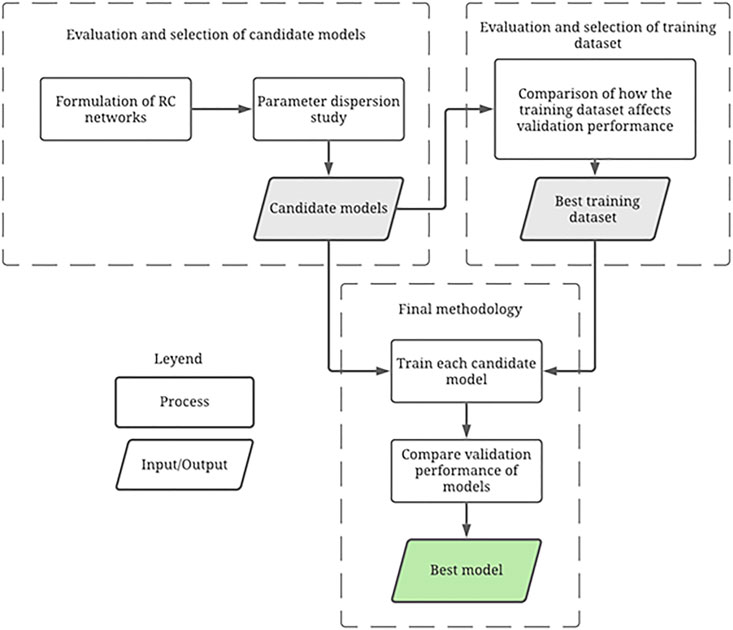
FIGURE 1. Workflow followed in this work.

2.1 Case studies

The case studies, one-story houses located in Panama, are built in DesignBuilder (DB), a graphical interface for EP. Case studies one and two are geometrically alike but differ in the materials used for construction. The thermal characteristics of each case study are summarized in Table 1. In any case, the house is occupied by one person all day. There are no elements surrounding the house that might mitigate solar radiation.

TABLE 1

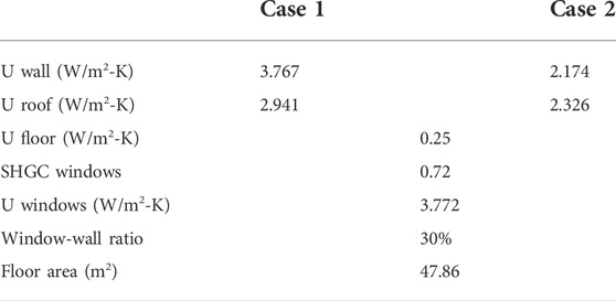
TABLE 1. Thermal properties for case studies.

The meteorological data used in DB consist of a typical year in Panama City. Each case study is studied under two operation regimes: passive regime, where windows are shut all day, and there is no air conditioning (AC), and active regime, in which an AC system is used according to a specified schedule. The house is equipped with a fan coil AC system, where the supply air mass flow rate is kept constant to maintain linearity in Eq. 4.

2.2 Training datasets

A dynamic simulation is run in DB to obtain the input and output data used for model training and validation. Four months are simulated: February (typically the driest month of the year), November (typically the rainiest), April, and December (2 months with intermediate climate conditions). These months are divided into twelve possible training datasets, varying in length, detailed in Table 2.

TABLE 2

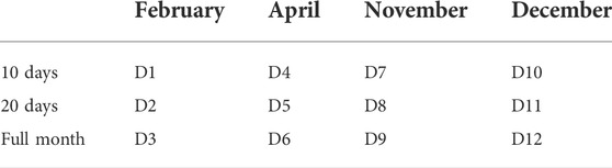
TABLE 2. Datasets for model identification.

2.2.1 Sampling interval selection

Careful selection of the sampling interval under which data is collected is important since data should be able to reflect the dynamic processes in the system. For the passive regime, preliminary parameter estimations show that a sampling timestep of 1 minute or 5 minutes results in consistent parameter estimates (pointing toward identifiable models). Therefore, the sampling interval for the passive regime is chosen as 5 min to work with the least amount of data.

For the active regime, however, the model is more sensitive to the timestep of data. In this mode of operation, the system is excited by the temperature setpoint of the AC system. The data must be able to reflect the evolution of temperature because of a change in temperature setpoint or AC state (on/off). The tested data sampling intervals were 1-min, 5-min, and 15-min. A preliminary study is conducted with a 15-min time step, the preferable sampling interval to work with the least of data and optimize identification. This timestep did not achieve good performance. It is possible that a timestep of 15 min lacks sufficient data points to model this behavior, rendering it unable to describe the change in indoor temperature when the AC changes state (from on to off or vice versa).

Ultimately, a 1-min time step is selected as the sampling time for data in the active regime. Preliminary model identifications with 1-min and 5-min timesteps result in RMSEs of 0.344 and 0.984°C, respectively, indicating that better performance can be achieved with data with a higher resolution. Moreover, analyzing the parameter estimates, only a 1-min timestep resulted in consistent parameters.

2.3 RC network design

The networks are designed in increasing complexity, starting from the simplest network, 1R1C, and successively adding states, resistances and/or inputs, up to the most complex network 4R3C. This workflow is shown in Figure 2. Networks with more than three states are not considered for two reasons: previous authors have found that the appropriate model order model a single-zone case study with a second or third-order network (Gray and Schmidt 2018; Rouchier et al., 2018; Wang and Chen 2019; Austin et al., 2020; Yang et al., 2020); and among the goals of this work is to identify a simplified model, i.e., with few parameters.

FIGURE 2

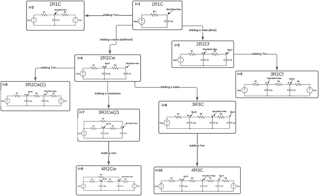
FIGURE 2. RC networks proposed.

2.3.1 States

Through the insights gathered from the literature review and case study knowledge, the states, and circuit nodes, considered for the networks include indoor air temperature (Ti), wall/roof temperature (Tw), and/or floor temperature. Indoor air temperature is included as a state in all candidate models, while in some networks, either wall/roof temperature or floor temperature, or both, are included. While indoor air temperature and wall/roof temperatures are commonly included as states in RC networks (Joe and Karava 2017; Gray and Schmidt 2018; Yang et al., 2018; Cui et al., 2019; Wang and Chen 2019; Wang J et al., 2019), floor temperature is less frequently observed. As in (Austin et al., 2020), the case studies to be modeled have a significantly thick concrete slab with thermal inertia that is important to consider in the thermal network.

2.3.2 Inputs

Model inputs are selected according to the literature review and the results of sensitivity analysis in DB. The building components that most affect indoor temperature are glazing type and external wall construction for both operation modes.

External wall construction can be associated with ambient temperature input since this is a boundary condition for the walls. This is an input considered by many authors in RC networks (Yang et al., 2018; Cui et al., 2019; Wang Z et al., 2019; Austin et al., 2020). On the other hand, glazing type can be associated with effective solar gains, which is the fraction of solar radiation transmitted through windows. Effective solar gains ($Qso{l}_j$) are incorporated in the model differently depending on the operating regime. For active mode, Qsol_j is given by Eq. 3, where F_j is the solar gain factor, and an estimated parameter and $\varphi$ is global horizontal irradiance (GHI), a model input that could be obtained from a weather station. The subindex j specifies the temperature nodes solar gains are affecting. For example, different effective solar gains could be associated with air, wall/roof, and floor temperatures, as seen in network 4R3C in Figure 2. For the passive regime, $Qsol$ is directly obtained from the available transmitted solar gains as calculated by DB. Instead of weather data, this value is used to design a control scheme that controls solar radiation transmitted through windows, such as the use of blinds of shading. This is proposed as further work.

$\begin{array}{c}Qso{l}_j=F_j\cdot \varphi \end{array}(3)$

Other inputs included in the proposed networks are internal gains and mean radiant temperature, both obtained from DesignBuilder. Internal gains represent heat gains by occupants or lighting equipment, considered as a constant input as in (Chen et al., 2016; Liu et al., 2016; Gray and Schmidt 2018; Yang et al., 2018; Wang J et al., 2019; Yang et al., 2020). Mean radiant temperature, while considered in (Yang et al., 2018) as a function of surface temperature and areas, in this work it is obtained directly from DB for simplicity and used to model radiative heat gains unaccounted by any of the inputs mentioned thus far.

In the active regime, a heat source is added to the network representing the heat extracted by the air conditioning system. This heat flow is given by Eq. 4, where known constants correspond to supply air mass flow and specific heat. G is an estimated parameter, and $T_s$ is the AC supply air temperature.

$\begin{array}{c}{Q}_{ac}=G\cdot \dot{m}\cdot Cp\left(T_s-T_i\right)\end{array}(4)$

2.3.3 State-space representation

Once the RC networks is designed, the equations that govern the network dynamics are obtained from a heat balance at each node of the RC network. This results in a set of ordinary differential equations (ODEs), which can be rearranged in space state representation. Eqs 5–8 show the ODEs that describe the dynamics of network 4R3C. These equations are then rearranged in state-space form, shown in Eq. 9. Model inputs, outputs, states, and parameters are summarized in Eqs 10–13.

$\begin{array}{c}{C}_i\frac{d{T}_i}{dt}=\frac{T_w-T_i}{R_2}+\frac{T_{mr}-T_i}{R_3}+Q_{sol1}+Q_{int}+Q_{ac}\end{array}(5)$

$\begin{array}{c}{\mathrm{C}}_w\frac{\mathrm{d}{\mathrm{T}}_w}{\mathrm{dt}}=\frac{{\mathrm{T}}_{out}-{\mathrm{T}}_w}{{\mathrm{R}}_1}-\frac{{\mathrm{T}}_w-{\mathrm{T}}_i}{{\mathrm{R}}_2}+Q_{sol2}\end{array}(6)$

$\begin{array}{c}\frac{\mathrm{d}{\mathrm{T}}_{\mathrm{i}}}{\mathrm{dt}}=-\frac{1}{{\mathrm{C}}_{\mathrm{i}}}\left(\frac{1}{{\mathrm{R}}_2}+\frac{1}{{\mathrm{R}}_3}+G\cdot \dot{m}\cdot cp\right){\mathrm{T}}_{\mathrm{i}}+\frac{1}{{\mathrm{R}}_2{\mathrm{C}}_{\mathrm{i}}}{\mathrm{T}}_w+\frac{G\cdot \dot{m}\cdot cp}{{\mathrm{C}}_{\mathrm{i}}}{T}_s+\frac{1}{{\mathrm{C}}_{\mathrm{i}}}{\mathrm{Q}}_{\mathrm{int}}+\frac{F_1}{{\mathrm{C}}_{\mathrm{i}}}\varphi +\frac{1}{C_i{R}_3}{T}_{mr}\end{array}(7)$

$\begin{array}{c}\frac{\mathrm{d}{\mathrm{T}}_w}{\mathrm{dt}}=\frac{1}{{\mathrm{R}}_2{\mathrm{C}}_w}{\mathrm{T}}_{\mathrm{i}}-\frac{1}{{\mathrm{C}}_w}\left(\frac{1}{{\mathrm{R}}_1}+\frac{1}{{\mathrm{R}}_2}\right){\mathrm{T}}_w+\frac{1}{{\mathrm{R}}_1{\mathrm{C}}_w}{\mathrm{T}}_{out}+\frac{F_2}{{\mathrm{C}}_{\text{i}}}\varphi \end{array}(8)$

$\left[\begin{array}{c}\frac{d{T}_i}{dt}\\ \frac{d{T}_w}{dt}\end{array}\right]=\left[\begin{array}{cc}-\frac{1}{{\mathrm{C}}_{\mathrm{i}}}\left(\frac{1}{{\mathrm{R}}_2}+\frac{1}{{\mathrm{R}}_3}+G\cdot \dot{m}\cdot cp\right)& \frac{1}{R_2{C}_i}\\ \frac{1}{R_2{C}_w}& -\frac{1}{C_w}\left(\frac{1}{R_1}+\frac{1}{R_2}\right)\end{array}\right]\left[\begin{array}{c}{T}_i\\ T_w\end{array}\right]+\left[\begin{array}{ccccc}0& \frac{G\cdot \dot{m}\cdot cp}{{\mathrm{C}}_{\mathrm{i}}}& \frac{F_1}{{\mathrm{C}}_{\mathrm{i}}}& \frac{1}{{\mathrm{C}}_{\mathrm{i}}}& \frac{1}{C_i{R}_3}\\ \frac{1}{R_1{C}_w}& 0& \frac{F_2}{{\mathrm{C}}_{\mathrm{i}}}& 0& 0\end{array}\right]\left[\begin{array}{c}{\mathrm{T}}_{out}\\ T_s\\ \varphi \\ {\mathrm{Q}}_{\mathrm{int}}\\ T_{mr}\end{array}\right](9)$

$\begin{array}{c}u={\left[\begin{array}{ccccc}{\mathrm{T}}_{out}& T_s& \varphi & {\mathrm{Q}}_{\mathrm{int}}& T_{mr}\end{array}\right]}^{\prime }\end{array}(10)$

$\begin{array}{c}y=T_i\end{array}(11)$

$\begin{array}{c}x={\left[\begin{array}{cc}{T}_i& T_w\end{array}\right]}^{\prime }\end{array}(12)$

$\begin{array}{c}\theta =\left[\begin{array}{ccc}{C}_i& C_w& \begin{array}{cccccc}{R}_1& R_2& R_2& F_1& F_2& G\end{array}\end{array}\right]\end{array}(13)$

2.3.4 Model identification

After the model structure is defined, parameter estimation is the next step in the system identification procedure. This work implements model identification in MATLAB’s System Identification Toolbox.

2.3.5 Parameter estimation

The two main functions used to formulate and solve the parameter estimation problem are: idgrey, which specifies the state-space model whose parameters should be identified; and greyest, the function that solves the nonlinear least-squares iteration problem using in each iteration the best search algorithm (Linear Grey-Box Model Estimation, 2022; Linear ODE Grey-Box Model with Identifiable Parameters, 2022). Model performance is assessed with the RMSE of indoor temperature in the validation dataset. Estimated parameters are thermal $C_i$, $C_w$, and $C_f$, corresponding to the thermal inertia of indoor air, wall/roof, and floor slab, respectively, thermal resistances $R_i$, and other coefficients such as $F_j$ and $G$.

2.3.6 Initial values and constraints

A critical component of the estimation problem is the parameter’s initial values. The closer the initial value is to the actual parameter values, i.e., the parameter that produces a global minimum, the faster the estimation problem is solved. It is also less likely for the algorithm to get stuck in local minima (Goodfellow et al., 2016). Moreover, the parameter value constraints could help guide the algorithm toward the possible solution. The initial values and parameter constraints are chosen according to domain knowledge.

For the estimation problem, the initial values of model capacitances are chosen randomly within 50% and 150% of an approximated physical value. This value is taken as the thermal mass of the corresponding building element. For resistances and solar gain factors, the initial values are random values between 1 and 0, while for G, it is between 1 and 2.

All parameters have a minimum constraint of zero since negative parameters have no physical meaning. The only parameters with a maximum constraint are thermal resistances since the actual values of thermal resistances of construction materials in the case studies are smaller than one.

2.4 Evaluation and selection of candidate models

The networks proposed in Figure 2 are selected or discarded according to a parameter dispersion criterion. We are only interested in identifiable models, meaning that there exists a unique parameter vector that produces a global minimum in the cost function (Ljung 1999). Therefore, the model’s parameter estimates must converge to a unique value regardless of its initial value. To study parameter estimates convergence, the following procedure is followed:

1) Train model ten times with D1 using a different initial value for every parameter in each identification.

2) Calculate de coefficient of variation (CV) for the ten parameter estimates.

3) Repeat steps 1 and 2 for datasets D2-D12.

4) Average the CV obtained for all datasets.

5) If the average CV of each parameter is smaller than or equal to 10%, the model is selected. Otherwise, it is discarded for its non-identifiability.

6) Repeat steps one to six for all models in Figure 2.

2.5 Evaluation and selection of training dataset

To determine the best training dataset for the model identification methodology, it is of interest to study the length of the training dataset and the month that produces the best model.

The models that were selected from the previous procedure each have twelve different identified versions, corresponding to estimates obtained from each of the twelve training datasets. Each of these versions is validated using the 3 months not used for training. The validation RMSE is averaged, and the training dataset that produced the lowest value is selected as the best training dataset for the methodology.

3 Results

In the following sections, the results of applying the procedures “Evaluation and selection of candidate models” and “Evaluation and selection of training datasets” in the passive and active regime are summarized.

3.1 Evaluation and selection of candidate models (applied to case 1 in active regime)

This section illustrates the candidate model selection procedure. Applying this procedure to the proposed models is shown for a selected network, a discarded network, and a network selected under special consideration. It is important to mention that for a model to be selected, its parameters must converge to a similar value in every iteration of the estimation process.

3.1.1 Selected model: 1R1C network

The model is trained ten times with different initial values for every parameter within the bounds established in section 2.3.6. The coefficient of variation is calculated for every parameter. Then, the twelve CVs for every estimated parameter are averaged. If each CV is under 10%, the model can be selected as a final candidate model. This is summarized in Table 3. It can be seen in Table 3 that 1R1C model is identifiable. Thus, it is selected as a candidate model for the final methodology.

TABLE 3

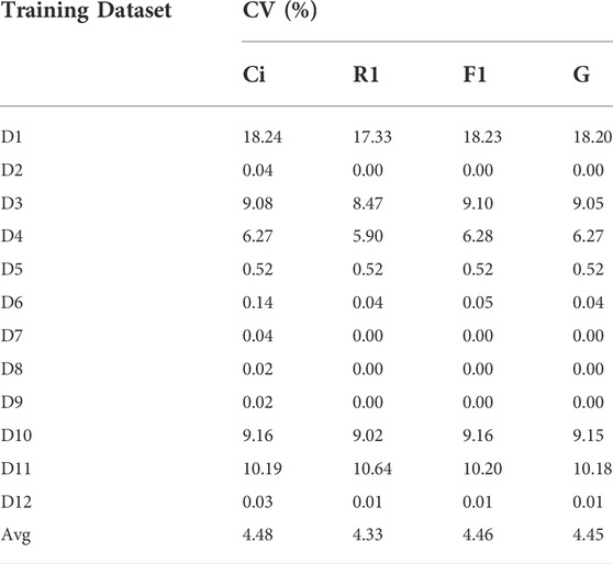
TABLE 3. Parameter dispersion in network 1R1C.

The results of applying the evaluation and selection of candidate models procedure to the network 1R1C when training with dataset D2 can be seen graphically in the scatter plot of Figure 3. Here, the ten random initial values for the indoor air capacitance Ci (which correspond to the data points that produce a higher RMSE, since the parameter is not chosen to be optimal) are matched to their corresponding estimated value, which was reached when the optimization was completed. The parameter reaches the same value regardless of its initial guess.

FIGURE 3

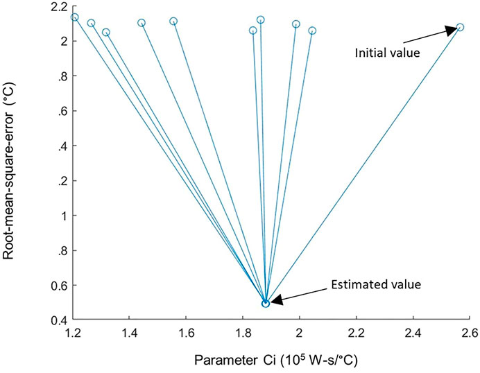
FIGURE 3. Initial vs. estimated values of parameter Ci when training with D2 in network 1R1C.

3.1.2 Model discarded: 2R1C network

As for the previous model, similar tables are generated for 2R1C network. The model is discarded because it does not meet the CV criterion. Figure 4 shows the scatter plot for parameter Ci when training with D1, confirming this conclusion.

FIGURE 4

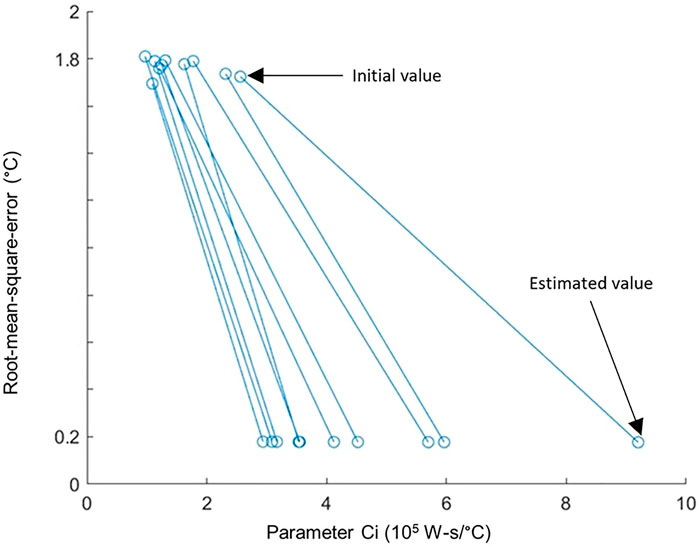
FIGURE 4. Initial vs. estimated values of parameter Ci when training with D1 in network 2R1C.

3.1.3 Model selected under special consideration: 2R2Cf network

A model that required further analysis was network 2R2Cf. During preliminary analysis, the network did not meet the dispersion criterion. However, upon closer study, it was found that only when training with D5 did the CV was over 10%; it was over 80%. This caused the average CV to be higher than 10%, leading the model to be discarded in the first instance. Figure 5 shows the scatter plot for parameter Ci when training with D5. Some estimations converge to a value with a higher RMSE than others, indicating that the algorithm may have gotten stuck on a local minimum for those estimations. Since there is a global minimum (around 0.3°C) only the estimations that converged to this value are considered. When the CV is recalculated for this dataset, the network does comply with the criterion and the model is selected as a candidate model for the final methodology.

FIGURE 5

FIGURE 5. Initial vs. estimated values of parameter Ci when training with D5 in network 2R2Cf.

3.1.4 Final candidate models

The final candidate models are the networks 1R1C and 2R2Cf; the rest are discarded for the active regime.

3.2 Evaluation and selection of training dataset (applied to case 1 in active regime)

Every final candidate model originates 12 models, one for every different training dataset available. The performance of each one is measured by averaging the validation RMSE using three validation datasets. These three validation datasets change depending on which training dataset is used. For example, if D1 is used for training, then D6, D9, and D12 are used for validating it. The training dataset that produces the best average validation performance produces a model with better generalization capabilities. The validation results for the networks 1R1C and 2R2Cf are shown in Table 4.

TABLE 4

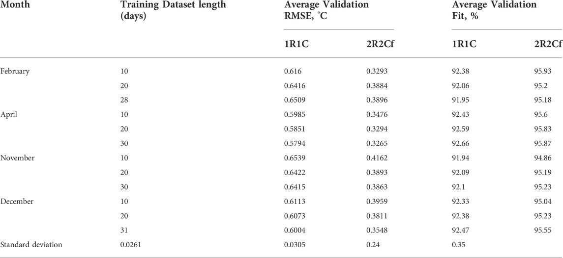
TABLE 4. Validation results for networks in the active regime for Case 1.

The best training dataset for the active regime appears to be 30 days in April. Nevertheless, considering the standard deviation of the RMSE across all training datasets is less than 0.04°C, any training dataset can provide sufficient insights into the thermal dynamics inside the residence to obtain good validation performance. This leads us to conclude that a model trained with 10 days to use the least amount of data of any month would be appropriate for the methodology in an active regime.

3.3 Evaluation and selection of candidate models (applied to case 1 in passive regime)

The only model that complies with the CV criterion for the passive regime is the 1R1C and is, therefore, the only candidate model in the final methodology.

3.4 Evaluation and selection of the best training dataset (applied to case 1 in passive regime)

For the passive regime, validation performance is slightly better when training with April and December. This can be ascribed to these months’ intermediate characteristics between rainy and sunny. Hence, the data is more informative than the rest of the training datasets. This leads us to conclude that a model trained with 10 days, to use the least amount of data, of April or December would be appropriate for the final methodology in the passive regime.

3.5 Final methodology

The methodology is formulated from the conclusions obtained in the previous sections. These are summarized in the flow diagram of Figure 6. The only candidate models for the active regime are the 1R1C and 2R2Cf networks. For the passive regime, only the 1R1C network is considered.

FIGURE 6

FIGURE 6. Final methodology.

The chosen length for the training dataset is 10 days of any month for the active regime and 10 days of April or December for the passive regime. This methodology will be applied to model Case 2 in active and passive regimes. The results shown in the following sections are generated using 10 days of December as a training dataset, for both operation regimes.

3.6 Methodology applied to case 2 in active regime

The methodology is now implemented to determine the best model representing Case study two during the active regime.

3.6.1 Parameter dispersion

The methodology’s first step consists of re-verifying that the model is identifiable. As it was done for Case 1, the model is trained ten times, and the parameter dispersion is analyzed. Both models show highly consistent parameter estimates (CV < 10%).

3.6.2 Validation and selection of the best model

The models are validated with datasets D3, D6 and D9 corresponding to the months of April, November, and December, respectively. Figure 7 plots the indoor temperature simulated by the 1R1C and 2R2f networks for two randomly chosen days in April and compares it with the DesignBuilder reference model data. For active regime, the best model is the 2R2Cf with an average RMSE of 0.3573°C.

FIGURE 7

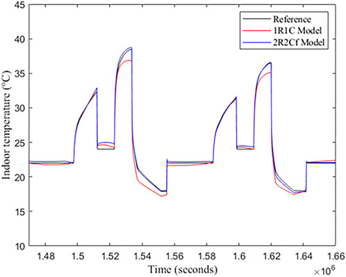
FIGURE 7. Simulated indoor temperature by models in active regime.

3.7 Methodology applied to case 2 in passive regime

3.7.1 Parameter dispersion

Parameter estimates dispersion for network 1R1C is reevaluated for the passive regime. The estimates meet the dispersion criterion (CV < 10%). Therefore, the model is validated.

3.7.2 Validation

During the validation, model 1R1C had an average validation RMSE of 0.9911°C. Figure 8 plots the internal temperature simulated by the 1R1C network for two randomly chosen days in November.

FIGURE 8

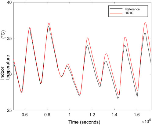
FIGURE 8. Simulated indoor temperature by model in the passive regime.

3.8 Development of a conceptual control system using the model identified for the active regime

The thermal models identified have as input the supply temperature of the air cooled by an air conditioning system that operates at a constant flow rate (e.g., mini-splits). This by itself is not a controllable input in real air conditioning systems; however, if there is a model that relates the supply temperature to some controllable variable (e.g., refrigerant flow) it could be feasible to design a controller with the identified model. However, this is outside the scope of this research. This section aims to use the gray box thermal model identified to design a conceptual control scheme where the manipulated variable is the supply temperature of the air conditioner, which is one of the model inputs.

The controller is designed in MATLAB Simulink with the assistance of the Control System Toolbox, taking the 2R2Cf model as the control loop plant. The controller gains are adjusted with the PID Tuner in MATLAB. The controller gains are automatically adjusted to achieve, on a step input, a settling time of approximately 300 s (5 min) and that the overshoot is below 15%. The controller’s performance is validated in a control loop that uses as a plant a black box state-space model obtained with N4SID, whose validation RMSE for 1 month of training was 0.218°C. Both control loops are shown in Figure 9.

FIGURE 9

FIGURE 9. Control loop implemented in Simulink.

In Figure 10 the response of both loops is plotted; the starting point is an initial condition of 21.59°C, and it is desired to achieve a set point of 18°C. In both responses, the design objective is achieved. The identified model can successfully be used to tune a controller that will control another plant, avoiding the need for a tedious trial and error procedure.

FIGURE 10

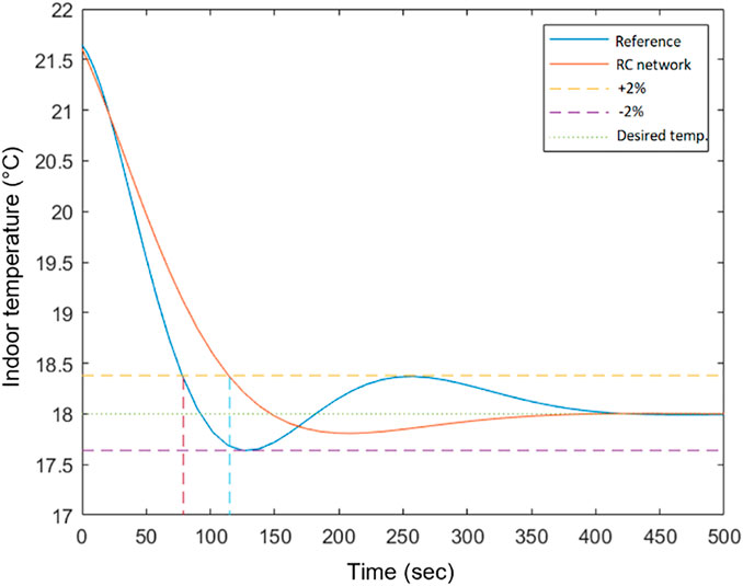
FIGURE 10. Closed-loop response.

4 Discussion

4.1 Active regime

The candidate models for this regime are networks 1R1C and 2R2Cf. These were the only identifiable models. Coincidentally, these were models with few parameters that resulted in an equal or better performance than models with more parameters. These results are similar to the conclusions presented by (Brastein et al., 2018). By reducing the number of free parameters in the estimation procedure, they could obtain consistent parameter estimates. The RC network with the best performance and physical interpretability in (Z. Wang and Chen 2019) also considered two states, indoor temperature and building envelope temperature. The latter state is comparable to floor temperature in the 2R2Cf network.

The model discarded 2R1C showed the particularity of always resulting in a null value for the parameter multiplying the global horizontal irradiance. One possible explanation is found by analyzing the Pearson correlation coefficient of inputs to outputs, shown in Figure 11. This network, unlike 1R1C, included mean radiant temperature as an input. The global horizontal irradiance and the mean radiant temperature are highly correlated with the output, indicating good estimators. However, the mean radiant temperature is a better estimator, having a higher correlation index. Since this temperature considers all the radiation exchanges between the surfaces of the building, it nullifies the effect of the global horizontal irradiance on the output.

FIGURE 11

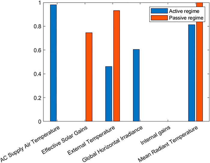
FIGURE 11. Pearson correlation coefficient for model inputs and outputs.

4.2 Passive regime

In the passive regime, the only identifiable model was the 1R1C. The data used for training in this regime corresponded to the free response of the building, without any cooling or heating to induce a forced response. It would seem a first-order model is accurate enough to emulate building dynamics sufficiently.

4.3 Training dataset characteristics

Results presented in sections 3.2, 3.4 indicate that model performance is not significantly affected by training dataset length or the weather conditions of the month during which data was collected. This could be related to the choice in modeling technique, a grey-box model. Since the model structure is based on physical equations, the model can generalize well regardless of the characteristics of the training data. This is an advantage of grey-box models over black-box models, where the latter are more dependent on the training dataset to achieve good generalization.

4.4 Comparison of operation regimes

The lowest average RMSE obtained for the active regime was 0.3573°C and for the passive 0.99°C. This means that the best active model has a RMSE almost 3 times less than the best passive model. This can be explained through the Pearson coefficient of inputs to outputs for both models, shown in Figure 11. In active regime, the variable most correlated with the output (used in the models selected as final candidates) is the supply temperature. In contrast, for the passive regime, it is the outside temperature. The superior performance of the model in active mode can be attributed to the fact that the input most correlated with the output is controlled by the imposed temperature setpoint. On the other hand, the most correlated variable in the passive mode is a measurable disturbance that presents stochastic characteristics that can decrease the final quality of the identified model.

4.5 Assessment of model performance

Model performance in this paper, as measured by fit, was over 20% greater than in (Wang and Chen 2019), where fit percentage was around 70%. The greater fit of the model in this research could be attributed to the data used for training and validation. While in this research data was obtained from a simulation software, in (Wang and Chen 2019) data was obtained by sensors, which introduces random behavior that could result in lower performance. The same effect of real data on model performance can be seen in (Brastein et al., 2018), where the simulation errors for indoor temperature, as measured by RMSE, were between 0.330 and 1.899 K, depending on the dataset used for training. The lowest average RMSE obtained in this research was 0.3573°C, which is comparable to the best performance obtained in (Brastein et al., 2018). However, it is of interest to study how model performance would be affected by data collected during real building operation and better compare the results. This is proposed as further work. Comparing the performance of the networks developed in this research to those of (Gray and Schmidt 2018), a study in which training data was obtained from a simulation software as well, the RMSEs obtained are similar, which serves to validate the methodology developed thus far.

4.6 Applicability of methodology

The models identified in this research were calibrated for prediction of indoor temperature in residential, single-zone buildings located in a tropical climate. Occupant behavior in these case studies was constant, and its influence on indoor temperature prediction was negligible, as seen in Figure 11. Air conditioner operating schedule and setpoint were fixed as well. The methodology was successfully able to identify a model with good performance in a case study with these characteristics, subjected to the same occupant behavior and air conditioner operation schedule. The main difference in Case 2 was building materials. Therefore, the applicability of the methodology to more geometrically complex case studies and subjected to variable occupant behavior and air conditioner use remains to be tested and is proposed as further work.

5 Conclusion

This paper proposes a methodology to identify thermal RC networks to model building dynamics in humid, hot, and rainy tropical climates. The models are developed towards their implementation in controller design; therefore, among the main objectives of the methodology is to identify models with few parameters to maintain computational efficiency. The methodology developed allows the identification of models for two operation regimes: active, for case studies with air conditioning, and passive, for case studies under free response.

Two residential case studies are analyzed, Case 1 and 2, which are geometrically identical but built with different materials. These models are built and simulated in DesignBuilder to obtain the input and output data needed for system identification. Case 1 is used to draw the most relevant conclusions to formulate the methodology, namely identifiable candidate models and training dataset characteristics. Once the methodology is established, Case 2 is used to test it.

The procedures to formulate the methodology first determine which networks are identifiable models from a pool of ten proposed networks. For the active regime, networks 1R1C and 2R2Cf were identifiable; for the passive regime, only the 1R1C network was identifiable. Therefore, these models are the candidate models for the methodology. The second procedure to identify the methodology consists of determining the optimal amount of training days and the month in which data should be collected. Results show that the models behave well regardless of the training dataset characteristics, which indicates that a model structure based on physical principles is less dependent on the data used for parameter estimation. It is concluded that data collected from any month of the year would achieve a good performance; however, training dataset length is restricted to 10 days to work with the least amount of data.

The methodology is then applied to Case 2 to identify which candidate models best describe the thermal dynamics of the residential building. The best model for the active regime is network 2R2Cf, with a validation RMSE of 0.3572°C. For the passive regime, the 1R1C network has a validation RMSE of 0.9911°C. This lower performance in the passive regime is attributed to the presence of disturbances, such as weather conditions, that the model cannot account for. Meanwhile, in an active regime, the output is most correlated to the supply air temperature of the air conditioner system, which is controlled by the imposed temperature setpoint. Once the network that best represents the case study is determined with the methodology, the model is used to tune a PID controller. The controller gains are calibrated with the RC network, and it can be successfully employed to manipulate the supply air temperature and achieve the desired indoor temperature, with a settling time of 5 minutes. Using the model to tune PID controller gains avoids the need for trial-and-error procedures.

Future work includes the integration of natural ventilation as model input and accounting for the influence of window aperture on indoor temperature—a critical weather parameter in tropical climates in humidity. Therefore, the coupling of the thermal model developed in this research with a hygric model is also of interest for future research. This research used the thermal model to tune a PID controller. However, future research will include the development of more control-based schemes, such as model predictive control, using the identified model.

Data availability statement

The raw data supporting the conclusion of this article will be made available by the authors, without undue reservation.

Author contributions

Introduction, figures and writing of most of the manuscript by AR and JS Original concept by MA Formal analysis, and editing by AR and JS Supervision and funding by MA.

Funding

This research was funded by a Panamanian Institution Secretaría Nacional de Ciencia, Tecnología e Innovación (SENACYT) https://www.senacyt.gob.pa/(accessed on 20 May 2022) within the projects FID18-056 and FIED19-R2-005, together with the Sistema Nacional de Investigación (SNI).

Acknowledgments

The authors would like to thank the Technological University of Panama and the Faculty of Mechanical Engineering and Faculty of Electrical Engineering for their collaboration, together with the Research Group ECEB (https://eceb.utp.ac.pa/, accessed on 20 May 2022).

Conflict of interest

The authors declare that the research was conducted in the absence of any commercial or financial relationships that could be construed as a potential conflict of interest.

Publisher’s note

All claims expressed in this article are solely those of the authors and do not necessarily represent those of their affiliated organizations, or those of the publisher, the editors and the reviewers. Any product that may be evaluated in this article, or claim that may be made by its manufacturer, is not guaranteed or endorsed by the publisher.

References

Afram, A., Janabi-Sharifi, F., Fung, A. S., and Raahemifar, K. (2017). Artificial neural network (ANN) based model predictive control (mpc) and optimization of HVAC systems: A state of the art review and case study of a residential HVAC system. Energy Build. 141, 96–113. doi:10.1016/j.enbuild.2017.02.012

CrossRef Full Text | Google Scholar

Amasyali, K., and El-Gohary, N. M. (2018). A review of data-driven building energy consumption prediction studies. Renew. Sustain. Energy Rev. 81, 1192–1205. doi:10.1016/j.rser.2017.04.095

CrossRef Full Text | Google Scholar

Anđelković, A. S., and Bajatović, D. (2020). Integration of weather forecast and artificial intelligence for a short-term city-scale natural gas consumption prediction. J. Clean. Prod. 266, 122096. doi:10.1016/j.jclepro.2020.122096

CrossRef Full Text | Google Scholar

Austin, M. C., Chang, I., Bruneau, D., and Sempey, A. (2020). “Assessment of different approaches to model the thermal behavior of a passive building via system identification process,” in Advances in automation and robotics research. Editors A. Martínez, H. A. Moreno, I. G. Carrera, A. Campos, and J. Baca (Cham: Springer International Publishing), 112, 185–193. Lecture Notes in Networks and Systems. doi:10.1007/978-3-030-40309-6_18

CrossRef Full Text | Google Scholar

Bilous, I., Deshko, V., and Sukhodub, I. (2018). Parametric analysis of external and internal factors influence on building energy performance using non-linear multivariate regression models. J. Build. Eng. 20, 327–336. doi:10.1016/j.jobe.2018.07.021

CrossRef Full Text | Google Scholar

Bourdeau, M., Zhai, X. Q., Nefzaoui, E., Guo, X., and Chatellier, P. (2019). Modeling and forecasting building energy consumption: A review of data-driven techniques. Sustain. Cities Soc. 48, 101533. doi:10.1016/j.scs.2019.101533

CrossRef Full Text | Google Scholar

Brastein, O. M., Perera, D. W. U., Pfeifer, C., and Skeie, N.-O. (2018). Parameter estimation for grey-box models of building thermal behaviour. Energy Build. 169, 58–68. doi:10.1016/j.enbuild.2018.03.057

CrossRef Full Text | Google Scholar

Çengel, Y. A., and Cimbala, J. M. (2018). Fluid mechanics: Fundamentals and applications. McGraw-Hill Education. New York, New York, United States.

Google Scholar

Chen, L., Basu, B., and McCabe, D. (2016). Fractional order models for system identification of thermal dynamics of buildings. Energy Build. 133, 381–388. doi:10.1016/j.enbuild.2016.09.006

CrossRef Full Text | Google Scholar

Cholewa, T., Siuta-Olcha, A., Smolarz, A., Muryjas, P., Wolszczak, P., Anasiewicz, R., et al. (2021). A simple building energy model in form of an equivalent outdoor temperature. Energy Build. 236, 110766. doi:10.1016/j.enbuild.2021.110766

CrossRef Full Text | Google Scholar

Cholewa, T., Siuta-Olcha, A., Smolarz, A., Muryjas, P., Wolszczak, P., Guz, Ł., et al. (2022). An easy and widely applicable forecast control for heating systems in existing and new buildings: First field experiences. J. Clean. Prod. 352, 131605. doi:10.1016/j.jclepro.2022.131605

CrossRef Full Text | Google Scholar

Cui, B., Fan, C., M, J., Mao, N., Fu, X., Jin, D., et al. (2019). A hybrid building thermal modeling approach for predicting temperatures in typical, detached, two-story houses. Appl. Energy 236, 101–116. doi:10.1016/j.apenergy.2018.11.077

CrossRef Full Text | Google Scholar

Derakhtenjani, A. S., Candanedo, J. A., Chen, Y., Dehkordi, V. R., and Athienitis, A. K. (2015). Modeling approaches for the characterization of building thermal dynamics and model-based control: A case study. Sci. Technol. Built Environ. 21 (6), 824–836. doi:10.1080/23744731.2015.1057060

CrossRef Full Text | Google Scholar

Drgoňa, J., Arroyo, J., Figueroa, I. C., Blum, D., Arendt, K., Kim, D., et al. (2020). All you need to know about model predictive control for buildings. Annu. Rev. Control 50, 190–232. doi:10.1016/j.arcontrol.2020.09.001

CrossRef Full Text | Google Scholar

Finck, C., Li, R., and Zeiler, W. (2019). Economic model predictive control for demand flexibility of a residential building. Energy 176, 365–379. doi:10.1016/j.energy.2019.03.171

CrossRef Full Text | Google Scholar

Foucquier, A., Robert, S., Suard, F., Stéphan, L., and Jay, A. (2013). State of the art in building modelling and energy performances prediction: A review. Renew. Sustain. Energy Rev. 23, 272–288. doi:10.1016/j.rser.2013.03.004

CrossRef Full Text | Google Scholar

Goodfellow, I., Bengio, Y., and Courville, A. (2016). Deep learning. MIT Press. Cambridge, Massachusetts, United States.

Google Scholar

Gorni, D., del Mar Castilla, M., and Visioli, A. (2016). An efficient modelling for temperature control of residential buildings. Build. Environ. 103, 86–98. doi:10.1016/j.buildenv.2016.03.016

CrossRef Full Text | Google Scholar

Gray, F. M., and Schmidt, M. (2018). A hybrid approach to thermal building modelling using a combination of Gaussian processes and grey-box models. Energy Build. 165, 56–63. doi:10.1016/j.enbuild.2018.01.039

CrossRef Full Text | Google Scholar

Harish, V. S. K. V., and Kumar., A. (2016). A review on modeling and simulation of building energy systems. Renew. Sustain. Energy Rev. 56, 1272–1292. doi:10.1016/j.rser.2015.12.040

CrossRef Full Text | Google Scholar

Hong, T., Wang, Z., Luo, X., and Zhang, W. (2020). State-of-the-Art on research and applications of machine learning in the building life cycle. Energy Build. 212, 109831. doi:10.1016/j.enbuild.2020.109831

CrossRef Full Text | Google Scholar

Hu, Q., Oldewurtel, F., Balandat, M., Vrettos, E., Zhou, D., Claire, J., et al. (2016). Building model identification during regular operation - empirical results and challenges, 2016 American Control Conference (ACC). 06-08 July 2016, Boston, MA, USA: IEEE, 605–610. doi:10.1109/ACC.2016.7524980

CrossRef Full Text | Google Scholar

Isermann, R., and Münchhof, M. (2011). Identification of dynamic systems. Berlin, Heidelberg: Springer Berlin Heidelberg. doi:10.1007/978-3-540-78879-9

CrossRef Full Text | Google Scholar

Joe, J., and Karava, P. (2017). Agent-based system identification for control-oriented building models. J. Build. Perform. Simul. 10 (2), 183–204. doi:10.1080/19401493.2016.1212272

CrossRef Full Text | Google Scholar

Kathirgamanathan, A., De Rosa, M., Mangina, E., and Finn, D. P. (2021). Data-driven predictive control for unlocking building energy flexibility: A review. Renew. Sustain. Energy Rev. 135, 110120. doi:10.1016/j.rser.2020.110120

CrossRef Full Text | Google Scholar

Li, X., and Jin, W. (2014). Review of building energy modeling for control and operation. Renew. Sustain. Energy Rev. 37, 517–537. doi:10.1016/j.rser.2014.05.056

CrossRef Full Text | Google Scholar

Linear Grey-Box Model Estimation 2022, “Linear grey-box model estimation - MATLAB greyest - MathWorks américa latina.” n.d. Available at: https://la.mathworks.com/help/ident/ref/iddata.greyest.html. Accessed May 14, 2022.

Google Scholar

Linear ODE Grey-Box Model with Identifiable Parameters 2022, “Linear ODE (Grey-Box model) with identifiable parameters - MATLAB - MathWorks américa latina.” n.d. Available at: https://la.mathworks.com/help/ident/ref/idgrey.html. Accessed May 14, 2022.

Google Scholar

Liu, W., Wang, H., Zhao, H., Wang, S., Chen, H., Fu, Y., et al. (2016). “Thermal modeling for energy-efficient smart building with advanced overfitting mitigation technique,” in 2016 21st Asia and South Pacific Design Automation Conference (ASP-DAC) (25-28 January 2016, Macao, Macao: IEEE), 417–422. doi:10.1109/ASPDAC.2016.7428047

CrossRef Full Text | Google Scholar

Ljung, L. (1999). System identification: Theory for the user. Hoboken, New Jersey, United States: Prentice Hall PTR.

Google Scholar

Paschke, F., and Zaiczek, T. (2018). Identification of dynamic models for the short-term temperature prediction in a single room. IFAC-PapersOnLine 51 (2), 79–84. doi:10.1016/j.ifacol.2018.03.014

CrossRef Full Text | Google Scholar

Rouchier, S., Rabouille, M., and Oberlé, P. (2018). Calibration of simplified building energy models for parameter estimation and forecasting: Stochastic versus deterministic modelling. Build. Environ. 134, 181–190. doi:10.1016/j.buildenv.2018.02.043

CrossRef Full Text | Google Scholar

Secretaría Nacional de Energía (2017). Plan energético nacional, 2015-2050. Ciudad de Panamá: Secretaría Nacional de Energía.

Google Scholar

Smarra, F., Jain, A., de Rubeis, T., Ambrosini, D., D’Innocenzo, A., and Mangharam, R. (2018). Data-driven model predictive control using random forests for building energy optimization and climate control. Appl. Energy 226, 1252–1272. doi:10.1016/j.apenergy.2018.02.126

CrossRef Full Text | Google Scholar

Tangirala, A. K. (2018). Principles of system identification: Theory and practice. Boca Raton, Florida, United States: CRC Press.

Google Scholar

Wang J, J., Tang, C. Y., Brambley, M. R., and Li, S. (2019). Predicting home thermal dynamics using a reduced-order model and automated real-time parameter estimation. Energy Build. 198, 305–317. doi:10.1016/j.enbuild.2019.06.002

CrossRef Full Text | Google Scholar

Wang Z, Z., Chen, Y., and Li, Y. (2019). Development of RC model for thermal dynamic analysis of buildings through model structure simplification. Energy Build. 195, 51–67. doi:10.1016/j.enbuild.2019.04.042

CrossRef Full Text | Google Scholar

Wang, Z., and Chen, Y. (2019). Data-driven modeling of building thermal dynamics: Methodology and state of the art. Energy Build. 203, 109405. doi:10.1016/j.enbuild.2019.109405

CrossRef Full Text | Google Scholar

Yang, S., Wan, M. P., Ng, B. F., Dubey, S., Henze, G. P., Chen, W., et al. (2020). Experimental study of model predictive control for an air-conditioning system with dedicated outdoor air system. Appl. Energy 257, 113920. doi:10.1016/j.apenergy.2019.113920

CrossRef Full Text | Google Scholar

Yang, S., Wan, M. P., Ng, B. F., Zhang, T., Babu, S., Zhang, Z., et al. (2018). A state-space thermal model incorporating humidity and thermal comfort for model predictive control in buildings. Energy Build. 170, 25–39. doi:10.1016/j.enbuild.2018.03.082

CrossRef Full Text | Google Scholar

Yang, X.-S. (2016). Nature-inspired optimization algorithms. Elsevier Science. Amsterdam, Netherlands.

Google Scholar

Zhao, H.-X., and Magoulès, F. (2012). A review on the prediction of building energy consumption. Renew. Sustain. Energy Rev. 16 (6), 3586–3592. doi:10.1016/j.rser.2012.02.049

CrossRef Full Text | Google Scholar