Finite element modeling for predicting sound insulation of fixed windows in a laboratory environment

1 Introduction

Noise is one of the major environmental problems, especially in urbanized areas. It can cause various health problems. For example, exposure to noise is known to be associated with sleep disorders with awakenings (Muzet, 2007). Also, it is reported that transportation and recreational noise affects blood pressure and hypertension (Petri et al., 2021). Among the problems caused by noise, reducing working performance caused by noise is also concerned: for example, learning impairment in schools associated with noise is studied (Minichilli et al., 2018). Considering these situations, noise abatement is of vital importance in built environments. One of the most efficient devices is improving the sound insulation performance of façades, particularly windows, which are often its weak points compared to other building components.

Therefore, developing windows with high sound insulation characteristics is necessary for comfortable and healthy indoor sound environments. The sound insulation performance of windows is generally tested using laboratory measurements such as those stipulated by ISO 10140 (ISO 10140-1, 2016). However, measurement-based evaluation entails high development costs to prepare test samples and to perform tests themselves. Therefore, numerical analyses such as the finite element method (FEM) and the boundary element method can key technologies to realize efficient development of high sound insulation windows. One can expect to reduce development costs and lead times. Numerical analyses present benefits for modeling the detailed structure of real windows and surrounding laboratory environment. However, computationally expensive vibroacoustics analyses are necessary for simulating sound transmission through windows to incorporate consideration of coupling between vibration fields in structural parts of windows and sound fields in surrounding laboratory environments, as well as in air gaps of multilayer structures. Computationally efficient modeling is an important but challenging objective that must be achieved for the prediction of sound insulation performance of windows and for other building components such as walls. Another means for predicting the sound insulation performance of windows is using theories (Sewell, 1970; Davy, 2009, 2010; Rindel, 2018; Cambridge et al., 2020; Santoni et al., 2020) for single-leaf and double-leaf partitions. A well-reviewed article (Santoni et al., 2020) describing theories for calculating sound transmission through partitions is available. Theoretical predictions, which are faster than numerical analyses, are useful to elucidate the fundamental mechanisms of sound transmission through partitions. However, their modeling capabilities are lower than numerical analyses. Furthermore, recently, a prediction method combined with a linear regression analysis to measure data and Cremer’s theory (Davy, 2009) have been explored as a practical prediction method used for single-glazed windows (Tsukamoto et al., 2021). The study described herein specifically examines vibroacoustics numerical modeling using FEM to predict random-incidence sound reduction indices (SRIs) of fixed windows in a laboratory environment.

Some earlier works have discussed the prediction accuracy of SRIs of actual windows or window-like structures using vibroacoustic FEM with comparison of measurement data. Soussi et al. (Soussi et al., 2021) conducted the prediction of SRIs of double glazing windows with a wooden frame at low frequencies up to 630 Hz using FEM. They tested the prediction accuracy of numerical models, calibrated with an experimental modal analysis, with comparison of measured values. Løvholt et al. (Løvholt et al., 2017) used FEM to simulate the sound transmission between two rectangular rooms via a lightweight wall with a double glazing window at very low frequencies below 100 Hz. A comparison with measured results revealed the importance of detailed modeling in the structural connection to obtain a better agreement of SRIs between the simulations and measurements. Mimura et al. (Mimura et al., 2022a) predicted SRIs of a scale model of a double window using FEM at 100 Hz to 5 kHz. Also, a comparison between FEM results and measured SRIs was made in cases with and without frame absorbers. They showed that superior agreement is obtained for a case with frame absorbers in all perimeters in the air cavity. They also demonstrated the importance of sound transmission modeling in the structurally connected parts in some poor prediction cases. Apart from SRI prediction of windows, some researchers (Papadopoulos, 2003; Arjunan et al., 2013, 2014; Wawezynowicz et al., 2014) have put great effort into predicting SRI of walls or composite panels. Accurate and efficient modeling is a challenging task because of the necessity for structure–acoustic analysis.

Nevertheless, almost all earlier works exploring SRI predictions of windows only examine prediction accuracy by FEM for single-sized windows and for a limited frequency range. Therefore, the applicability of FEM to SRI predictions of real windows having different sizes remains unclear. Because actual dwellings use various-sized windows and because their sound insulation performance is influenced by the window or plate size (Guy et al., 1985; Mimura et al., 2022b), the prediction accuracy of SRIs using FEM should be examined for windows of multiple sizes. Furthermore, as described earlier, SRI predictions of windows using FEM in a wide frequency range require great computational effort when a detailed structure of the window is modeled. For that reason, exploring computationally efficient modeling of real window systems is expected to enhance the applicability of numerical analyses to window system design with a high sound insulation performance.

For the reasons described above, this study was conducted to elucidate the efficient and accurate finite element modeling for predicting SRI of fixed windows at random incidence in a laboratory environment. Therefore, we discuss the predictive accuracy and required computational costs of three FEM models for predicting random incidence SRI of fixed windows by comparing the measured SRIs of five fixed windows having different sizes of 0.2–2.0 m². We only specifically examine numerical models that discretize the window part or windows part and the space around the windows for computational efficiency reasons. In that model, source and receiving reverberation rooms are not discretized with finite elements. This paper is organized as follows. In Section 2, we evaluate the accuracy of the simplest numerical model that discretizes only a window part with finite elements under two loss factor setups that contribute to energy loss of vibrations in windows. One uses measured frequency-dependent total loss factors, as measured respectively for five windows. Sound incidence conditions to window surfaces are assumed as an ideal diffuse sound incidence. The acoustic radiation to an opposite transmission field is computed using Rayleigh’s integral. Then, Section 3 examines effects of including a niche in the numerical model on the resulting accuracy of SRI predictions at frequencies below 1 kHz because the discrepancies from measured SRIs can be found at this frequency range in Section 2, especially for smaller windows. Section 4 explores the applicability of the weak-coupling model to predict SRI for a numerical model with a niche more efficiently. Section 5 concludes the presentation, giving some important perspectives on creating an accurate and efficient numerical model to predict random-incidence SRI of fixed windows in a laboratory environment.

2 Prediction using model with window part only

This section presents a discussion of the prediction accuracy of SRI using a numerical model that discretizes only the window parts with finite elements for five fixed windows having different sizes of 0.2–2.0 m². The considered fixed windows are all used in actual dwellings. In the numerical model, an ideal diffuse field incidence condition is applied to the incident window surface. Also, acoustic radiation from the window surface on the transmitted side is computed using Rayleigh’s integral. Two numerical models, each with a different loss factors setup, were tested. The first setup gives an internal loss factor to each material. The second setup gives a measured total loss factor having frequency-dependence to window glazing. We examined the accuracy of the numerical model by comparing it with measured SRIs in laboratory measurements described in the authors’ earlier work (Mimura et al., 2022b). For readers’ convenience, we explain the measurement briefly in Section 2.1.

2.1 Measurement outline

Measurements were taken in two irregularly shaped reverberation chambers following JIS A 1416 (JIS A 1416, 2000), which is comparable to ISO 10140–1 (ISO 10140-1, 2016). The source reverberation room has a volume of 492.8 m³ and the receiving room has 264.5 m³ volume. We measured SRIs and the total loss factors of five fixed windows with area of 0.2–2.0 m². Figure 1A,B portrays a photo of the interior appearance of the reverberation room and a block diagram of the SRI measurement, respectively. Figure 2 presents a tested, fixed window of W × H size settled in an opening between two reverberation rooms. Those windows comprise glass, window frames of aluminum and PVC, and the gasket. Each window uses a float glass of 5 mm thickness. Table 1 presents detailed dimensions of five fixed windows (A)–(E) appearing in Figure 2 as the window size W × H, the glass size W_FL5 × H_FL5, the exposed glass size W_g × H_g, area and the aspect ratio. The windows were first attached to a sufficiently high-density wooden frame that had been filled with mortar inside. Then the resulting window component was mounted to the test opening. The measurements were taken in airtight conditions. We sealed the air gaps between the wooden frame and the opening with clay and sealed the air gaps between the wooden frame and window frame with tape.

FIGURE 1

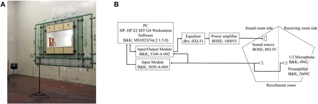
FIGURE 1. SRI measurement of window D: (A) interior appearance of source room and (B) a block diagram of measurement equipment.

FIGURE 2

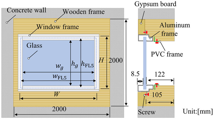
FIGURE 2. Appearance of fixed window using in measurements.

TABLE 1

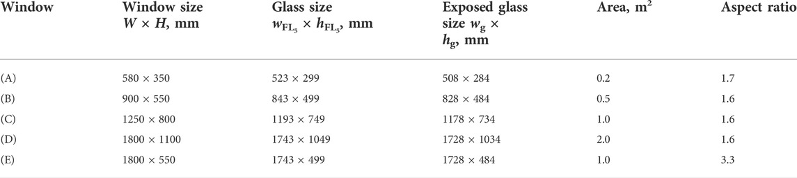
TABLE 1. Dimensions of five fixed windows.

We also took the total loss factor η_tot measurements to consider effects of boundary loss simply in the numerical model. Figures 3A, B portrays a photo of the impulse test and a block diagram of the equipment set-up for the measurement, respectively. The η_tots for five fixed windows (A)–(E) were calculated, respectively, from a structural reverberation time T_s, as measured using an impulse test with a steel ball pendulum. The accelerometers were mounted on the glass surface with small amounts of wax to fix them on the surface. The T_s is a value taken from averaging five times measuring results with three excitation points and three measured positions. Figures 4A, B respectively depict results of random incidence SRIs, in addition to the total loss factors for five fixed windows.

FIGURE 3

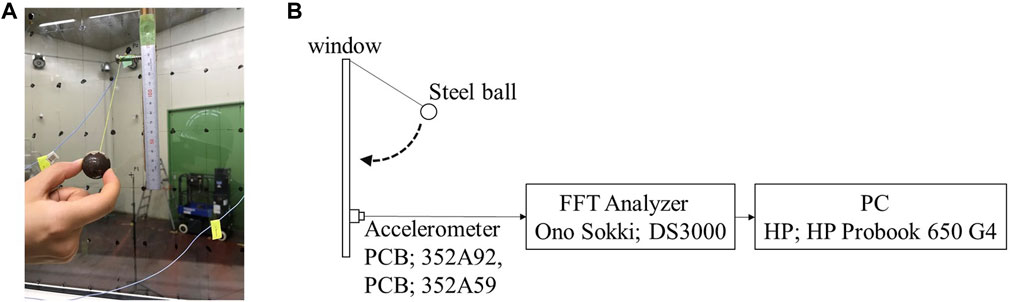
FIGURE 3. Total loss factor measurement: (A) a picture of impulse test and (B) a block diagram of measurement equipment.

FIGURE 4

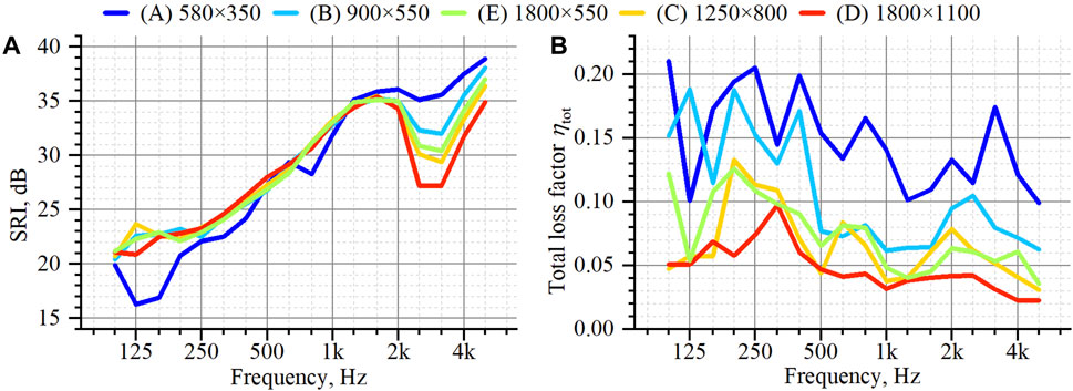
FIGURE 4. Measurement results of five fixed windows, (A) Sound reduction indices, and (B) Total loss factors (Mimura et al., 2022b).

2.2 Finite element model

We performed FEM simulations using vibroacoustic simulation software: Actran 2020. Simulations were performed at 1/24-octave band center frequencies of 90 Hz to 5.6 kHz in the frequency domain to predict the respective SRIs for the five fixed windows (A)–(E) having different dimensions. The calculation results were evaluated as 1/3-octave band SRIs at 100 Hz–5 kHz. A linear direct frequency response analysis was used. A linear system of equations at each frequency was solved with a sparse direct solver called MUMPS. Figures 5A, B show the simplest and the baseline model that discretizes the window part with finite elements. The discretized model comprises aluminum and PVC frames, a glass, rubber sheet instead of a gasket, and an air cavity within the frames. Simplified geometries in a rubber sheet and window frame were used because they have complicated geometries. In the vibroacoustic simulation, the structural domains, aluminum and PVC frames, a glass, and a rubber sheet, are described by the differential equation of motion for a continuum body assuming only slight deformation as (Sandberg et al., 2008)

${\tilde{\nabla }}^{\text{T}}{\tilde{\mathit{\sigma }}}^{\text{s}}+{\mathit{b}}^{\text{s}}={\rho }^{\text{s}}\frac{{\partial }^2{\mathit{u}}^{\text{s}}}{\partial t^2},(1)$

where ρ^s is the density of material, ${\tilde{\mathit{\sigma }}}^{\text{s}}$ is the stress vector in Voigt notation, b^s is the body force vector, u^s is the displacement vector. With the strain vector ${\tilde{\mathit{\epsilon }}}^{\text{s}}$ represented by Voigt notation, the strain-displacement relation is written as

${\tilde{\mathit{\epsilon }}}^{\text{s}}=\tilde{\nabla }{\mathit{u}}^{\text{s}}.(2)$

FIGURE 5

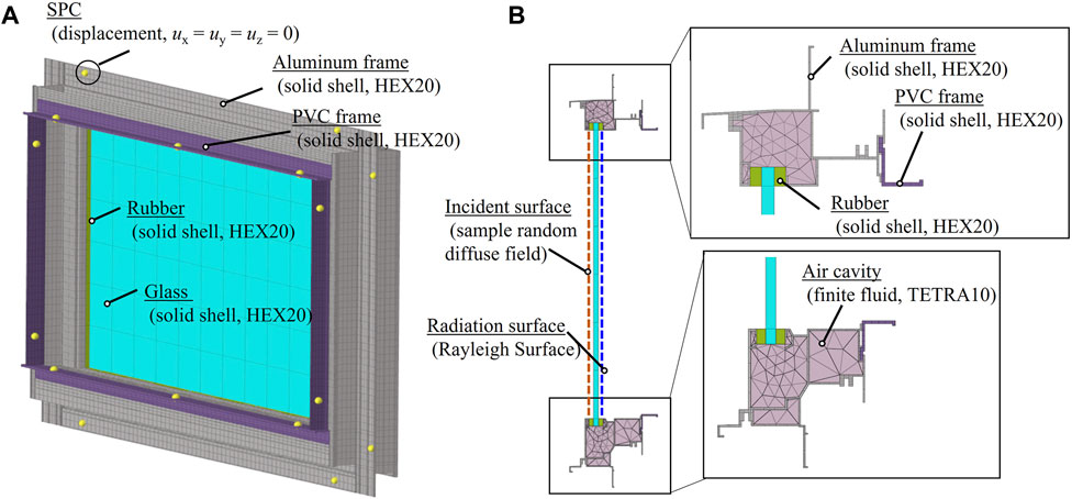
FIGURE 5. Numerical fixed window model discretized with solid shell elements in structural domains and fluid elements in acoustic domain for window: (A) Overall view, and (B) Cross-sectional view.

The stress-strain relation is given for an isotropic material as

${\tilde{\mathit{\sigma }}}^{\text{s}}=\mathit{D}{\tilde{\mathit{\epsilon }}}^{\text{s}},(3)$

where ${\tilde{\mathit{\sigma }}}^{\text{s}}={[{\sigma }_{11}^s{\sigma }_{22}^s{\sigma }_{33}^s{\sigma }_{12}^s{\sigma }_{13}^s{\sigma }_{23}^s]}^{\text{T}}$, and ${\tilde{\mathit{\epsilon }}}^{\text{s}}={[{\epsilon }_{11}^s{\epsilon }_{22}^s{\epsilon }_{33}^s{\gamma }_{12}^s{\gamma }_{13}^s{\gamma }_{23}^s]}^{\text{T}}$. The constitutive matrix D is described as

$\mathit{D}=\left[\begin{array}{cccccc}\hfill \lambda +2\mu \hfill & \hfill \lambda \hfill & \hfill \lambda \hfill & \hfill 0\hfill & \hfill 0\hfill & \hfill 0\hfill \\ \hfill \lambda \hfill & \hfill \lambda +2\mu \hfill & \hfill \lambda \hfill & \hfill 0\hfill & \hfill 0\hfill & \hfill 0\hfill \\ \hfill \lambda \hfill & \hfill \lambda \hfill & \hfill \lambda +2\mu \hfill & \hfill 0\hfill & \hfill 0\hfill & \hfill 0\hfill \\ \hfill 0\hfill & \hfill 0\hfill & \hfill 0\hfill & \hfill \mu \hfill & \hfill 0\hfill & \hfill 0\hfill \\ \hfill 0\hfill & \hfill 0\hfill & \hfill 0\hfill & \hfill 0\hfill & \hfill \mu \hfill & \hfill 0\hfill \\ \hfill 0\hfill & \hfill 0\hfill & \hfill 0\hfill & \hfill 0\hfill & \hfill 0\hfill & \hfill \mu \hfill \end{array}\right].(4)$

The Lamé coefficients λ and μ are defined as

$\lambda =\frac{\nu E}{\left(1+\nu \right)\left(1-2\nu \right)},(5)$

$\mu =\frac{E}{2\left(1+\nu \right)},(6)$

where E is the Young’s modules, and ν is the Poisson’s ratio. The acoustic domain, the air in the air cavity, is described with the lossless wave equation as

$\frac{{\partial }^{2}p}{\partial t^2}-c^2{\nabla }^{2}p=0,(7)$

where p is the sound pressure, and c is the speed of sound in air. The coupling condition at the boundary between structural and acoustic domains is given by the displacement boundary condition and the continuity in pressure as

$u^s{|}_n=u^a{|}_n,(8)$

${\sigma }^s{|}_n=-p,(9)$

where u^a is the fluid displacement at the interface, and n is the normal vector. The computations were performed in frequency domain using a computer (Proliant DL380; HP Inc., Xeon(R) CPU E5-2690 v4 @ 2.60 GHz, 28 cores; Intel Corp.). The calculations were done using four processes with IntelMPI parallel computation. The parallel computations were performed in a frequency direction. For example, four pure tone analyses were performed in parallel when using four processes. Using this strategy, four times the memory must be used compared to that used for serial computations.

We created three FE meshes, each having a different spatial resolution according to the analyzed frequency range for efficient computation. To account for vibration fields in structural domains, the glass, the aluminum and PVC frames, and the rubber sheet were discretized with three-dimensional solid shell HEX20 elements, which are twenty-node second-order hexahedron solid shell element (Petyt, 2010; Free Field Technologies, 2019) with three degrees of freedom at each node for the displacement u_x, u_y and u_z in x-, y- and z-axes. The solid shell elements can avoid thickness-locking and shear-locking effects. The element size for the window frames was set as 10 mm, irrespective of the analyzed frequency, which corresponds to one-fourth of the bending wavelength in the aluminum frame at 5 kHz. It is noteworthy that we use the same sized elements for the PVC frame, although a smaller element size might be necessary when considering its bending wavelength. For this study, we assumed that this choice has a minor role in affecting the results because the proportion of PVC frames is much smaller than the aluminum frame, as shown in Figure 5. For glass and rubber, their element sizes are one-fifth smaller than the bending wavelength of the glass. Although the rubber needs a smaller element size, we used the same size as in the glass, assuming that rubber deforms along with the glass. For these window frames, and the glass and rubber, the number of elements in their thickness direction was one. We used three-dimensional TETRA10 finite fluid elements, the second-order ten-node tetrahedron elements, for the air cavity inside the window frames. Moreover, we set the element length as less than 20 mm at all frequencies, corresponding to one-third of the acoustic wavelength at 5 kHz. As might be apparent in Figure 5B, we used non-congruent meshes to deal with different element sizes and different element types in each structural domain and acoustic domain efficiently. The aluminum frame is discretized with HEX20 solid shell elements and the air inside the frame is discretized with TETRA10 finite fluid elements having different element size as in the solid shell elements. Therefore, the interface connection (Free Field Technologies, 2019) was used to consider mutual propagation between domains having different element types and sizes at those interfaces. The interface connection formulates coupling constraints by projecting nodes on the coupling surface to another surface. The displacement continuity is maintained in the structure–structure connection. The total node numbers in the baseline model were approximately 240,000–534,000 for windows (A)–(E).

Regarding the sound-incidence condition to the window surface, we used an Actran component, the sampled random diffuse field (Wittig and Sinha, 1975; Van den Nieuwenhof et al., 2010; Coyette et al., 2014; Free Field Technologies, 2019), to simulate a diffuse-incidence condition. Two sampling methods can be selected for a diffuse field in the component. The first is a method based on a Cholesky decomposition of the cross PSD matrix. The present discussion is an assessment of using this first method. The second is a method based on a superposition of many discrete plane waves. The second approach is used for the explanations presented in Section 3 and Section 4. To calculate SRI at random-incidence, the maximum sound incidence angle is assumed to be 78°. The acoustic radiation from the window was computed with a Rayleigh surface (Kirkup, 1994; Free Field Technologies, 2019). The SRI is calculated as

$\mathrm{S}\mathrm{R}\mathrm{I}=10\mathrm{l}\mathrm{o}{\mathrm{g}}_{\mathrm{10}}\left(W_{\text{inc}}/W_{\text{rad}}\right),(10)$

where W_inc represents the incident sound power computed from the spatial correlation on the glass surface. The radiated sound power W_rad is calculated using Rayleigh’s integral of vibration velocities on the glass surface, including air resistance. For the diffuse field incidence condition, we set the sample number as 40. This sample number choice is based on results obtained from our earlier work (Mimura et al., 2022a), where the deviation in SRI on the use of this sample number from 100 sample number results was only 0.3 dB. In the numerical window model, screws are represented by clamped boundary conditions as a support condition (SPC). For the solid shell elements, this boundary condition is expressed as follows: three displacement components u_x, u_y and u_z were set to be zero at the node positions of the screws, as shown in Figure 5A. Table 2 presents the number of screws for the five fixed windows. They differ among the respective windows.

TABLE 2

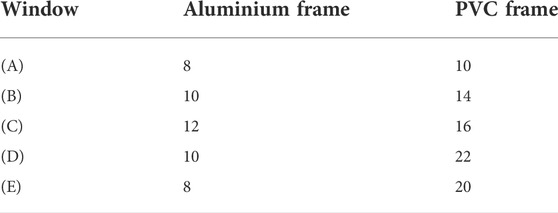
TABLE 2. Number of screws attaching the window frame.

Table 3 presents the material properties of the glass, aluminum, PVC, rubber, and air. We used the calibrated Young’s modulus for rubber with the measured results of window (A) so that the first modal frequency in the analysis matches the measured first modal frequency. Because the actual rubber material used for real windows is a hollow material, the adjusted Young’s modulus for the numerical model is smaller than the general values. Table 3 shows that we used two loss factor setups for the numerical model: Type 1 and Type 2. Type 1 uses an internal loss factor η_int of each solid material as a complex Young’s modulus, in which the η_ints of the glass and PVC were obtained using a preliminary experiment with the central excitation method. For the rubber and the aluminum, their η_ints were set to values included in Actran’s material library. However, Type 2 uses the measured frequency-dependent total loss factor η_tot, as shown in Figure 4B to the glass. Here, we considered that the measured total loss factor expresses the vibration energy loss of glass including losses from the connections to the surrounding structure. It was given as an effective loss factor of materials.

TABLE 3

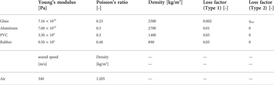
TABLE 3. Material properties.

2.3 Results

Figures 6A, B respectively portray SRI values computed using the simplest model in the upper panel and absolute errors from measurements in the lower panel for five fixed windows in applied loss factor setups of Type 1 and Type 2. Figures 6A, B, respectively present results for Type 1 and Type 2. We first qualitatively evaluate whether the numerical results reproduced the measured SRIs of fixed windows of different sizes. Two numerical results show consistent behavior with the measured SRIs in Figure 4A for the magnitude relation of SRIs above the coincidence frequencies and show a dip in window (A) because of the first mode. However, both numerical results clearly show size-dependent SRIs below 400 Hz for windows (B)–(E). In those cases, smaller windows show larger SRI. Although the size-dependent SRI for the numerical results is explainable by the difference of radiation efficiency coming from the window dimensions, this size-dependent effect cannot be observed in the measured results. We infer that this difference between numerical results and measured results might derive from the fact that FEM predictions assumes an ideal diffuse incidence conditions and that it does not consider actual incidence conditions in the laboratory environment. However, detailed investigations are left as a subject for future study. Regarding differences in numerical results between the two loss factor setups, results show suggest that the resulting SRI difference occurs mainly at the first normal mode of window (A) and around and above the coincidence frequency for all windows. For the minimum sized window (A), the SRI computed using Type 1 shows a deeper dip at 125–160 Hz, which derives from the first normal mode of the window, than for SRI computed using Type 2. Some fluctuations are apparent below 160 Hz for the largest-sized window (D) when using the setup of Type 1. Additionally, the SRIs computed using Type 2 show higher SRI values than those using Type 1 above the coincidence frequencies. The boundary loss factor can be said to have a strong effect on the resulting SRI values above the coincidence frequencies because the presented windows have low internal loss factors for the respective solid materials.

FIGURE 6

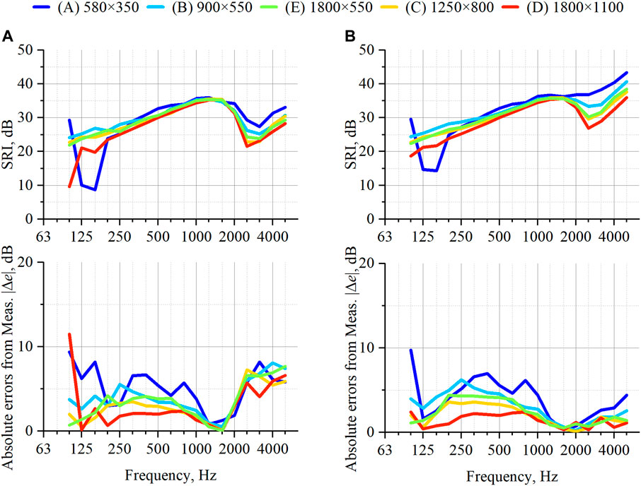
FIGURE 6. Comparison of (Upper) SRIs for five fixed windows computed by FEM with different loss factor setup and (Bottom) absolute difference from measured SRIs: (A) result obtained using internal loss factor setup and (B) results obtained using measured total loss factor.

Furthermore, from a quantitative perspective, the numerical results obtained using Type 2, which uses η_tot as an effective loss factor of material, show better agreement to the measured SRIs at the first normal mode for window (A) and around and above the coincidence frequencies for all windows, as might be apparent from the lower panels of Figure 6. The absolute errors of the results obtained using Type 2 are 0.1–4.4 dB, whereas those of the results obtained using Type 1 show larger errors of 4.0–8.2 dB. The absolute errors in Type 2 results become smaller for larger windows. We also confirmed for numerical models using Type 1 and Type 2 that there is a difference in vibration attenuation on the glass surface at the first normal mode and at frequencies above the coincidence frequencies. Large vibration amplitude was observed at the coupling interface between the rubber and the aluminum frame for those frequencies, which indicates that boundary losses can contribute an important influence at those frequencies. The numerical model using Type 2 includes this boundary loss effect. Therefore, it was able to show higher accuracy than the numerical model using Type 1. Although the total loss factor remains an unknown value at a design stage, our earlier study (Mimura et al., 2022b) revealed that its frequency-averaged value shows a linear relation with the parameter $\frac{U}{S}$ of windows, where U and S represent the window perimeter and area, which indicates the possibility of predicting the total loss factor of different-sized windows. This possibility will be explored further in our future studies. However, both numerical results obtained using Type 1 and Type 2 show large absolute errors below 1 kHz for smaller-sized windows. At that frequency range, numerical results show overestimation of the measured SRI values. We infer that this discrepancy mainly derives from neglecting the niche in the simplest numerical model used in this section because the numerical results show larger discrepancies from the measured results for smaller windows at frequencies below the coincidence frequency, which indicates that the SRI of the measured results might be reduced by the niche effect (Kim et al., 2004; Vinokur, 2006; Sakuma et al., 2017). The next section will elucidate whether the modeling of niche engenders improved SRI predictions.

Regarding the computational cost of this baseline model which discretizes the window part only, total computational times were 9,491 s and 27,443 s, respectively, for the smallest window (A) and the largest window (D). The maximum memory requirements for the window (A) and (D) models were, respectively, 13.5 and 44.9 GB per process. Those results indicate that the necessary computational costs for the baseline model are acceptable and sufficiently practical in recent computational environments.

This section describes that using a measured total loss factor yields higher prediction accuracy at the first normal mode and around and above coincidence frequency than using internal loss factors.

3 Improvement by including a niche

This section presents discussion of whether or not including a niche into the numerical model produces better agreement with the measured SRI for five fixed windows. The examination specifically emphasizes SRI below 1 kHz, for which large discrepancies from the measured results were observed. The numerical model used for this examination requires assumption of a diffuse sound incidence condition, but hemispherical free spaces around the window are discretized by finite fluid elements combined with infinite elements. In doing so, the niche in a laboratory environment is included in the numerical model. For the discussion presented herein, Type 2 loss factor setup using measured η_tot is used because this setup showed better accuracy in the preceding section.

3.1 Strong-coupling model

Figure 7 portrays the numerical model with a niche in which the fixed window part uses the same discretized model in Figure 5. However, this model further discretizes the sound incidence field and radiating sound field around the fixed window as hemispherical free spaces to model the niche. The structure–acoustics coupling between the sound fields around the windows and vibration fields in windows are considered. A strong-coupling model is used for the explanation presented in this section. Because this model considers free field sound radiations around the window, infinite elements are used on the hemispherical surfaces. The sound fields in the hemispherical spaces are discretized by TETRA10 second-order finite fluid elements. The element sizes were set below 114 mm, thereby satisfying element size of less than one-third of the acoustic wavelength at 1 kHz. The radius of the hemisphere spaces is 1.4 m, corresponding to four times the wavelength at 1 kHz. We use a non-congruent mesh for this model. The hemispherical sound fields and windows are connected by the interface connector. As an infinite element, an Actran component, infinite fluid (Free Field Technologies, 2019; Astley and Coyette, 2001a,b), was used on the hemisphere surfaces to reproduce free-field sound radiation. With this component, the sound radiation to infinite distance is calculated based on the sound distance attenuation, using a complement factor in radius direction including the Sommerfeld condition and the coordinate system of the acoustic field. To realize the diffuse sound-incidence condition, the sampled random diffuse field component is again used on the outside surface of the hemisphere on the incident side, but the method based on the superposition of numerous plane waves at random phase is used here. The number of sampled random diffuse fields was set as 40. More than 8,000 plane waves were summed to reproduce a diffuse sound field. The maximum incident angle was set to 90°. The SRI was calculated using Eq. 10. The incident sound power W_inc was calculated on the glass surface of the incident side. The radiated sound power W_rad was calculated on the infinite fluid surface of radiating side. Actually, this model naturally has many more degrees of freedom than the baseline model used in the preceding section because of the discretization requirement of sound fields around the window. The total node numbers of the strong-coupling models were 1,080,977–1,963,834, respectively, for windows (A)–(E). Comparison of the node numbers of the baseline model shows that the strong-coupling models require approximately four times more nodes.

FIGURE 7

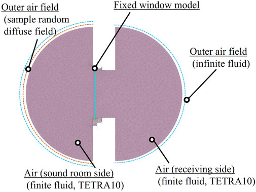
FIGURE 7. Strong-coupling model including the niche.

3.2 Results

Figure 8 portrays the SRIs computed using the numerical model with the niche for five fixed windows and absolute errors from measurements, respectively, in the upper and lower panels. Compared to the model results that discretize only the window part in Figure 6B, the present model results with the niche produce much better accuracy at 125 Hz–1 kHz for all windows. Considered quantitatively, the absolute errors by the numerical model with the niche are smaller than 3.3 dB, except for the results obtained for window (A) at 100 Hz. One can find that inclusion of the niche improves prediction accuracy in a laboratory environment for smaller windows. For the smallest window (A), the absolute errors from the measured result become less than 1.5 dB at 125 Hz–1 kHz. In addition, the numerical result of window (A) reproduces small dips at 315 and 800 Hz, which are found in the measured results. This result suggests that these small dips in the measurement derive from the niche effect. Based on those results, probably the niche effect is the primary reason for discrepancies using the baseline model from the measurement below 1 kHz, especially for smaller windows. Therefore, we can propose that the niche should be modeled in a numerical model to predict the SRI of fixed windows in a laboratory environment accurately. However, a large discrepancy exceeding 5 dB from the measured SRI can still be found at 100 Hz for the smallest window (A). This discrepancy in the stiffness control region might be derived from the numerical model that still does not include the source and receiving reverberant rooms. This is left as a subject to be addressed in our future work.

FIGURE 8

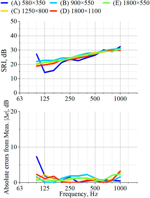
FIGURE 8. Results obtained using the strong-coupling model (Upper) SRIs for five fixed windows and (Bottom) absolute difference from measured SRIs.

Furthermore, using a strong-coupling model with a niche entails remarkably high computational costs. For instance, the computational cost in the minimum window (A) and the maximum window (D) were 60,432 s and 358,201 s in computational times. Moreover, windows (A) and (D) models respectively require 79 and 204 GB per process. It is noteworthy that the computations were made under two process parallel computations and a serial computation for window (A) and window (D) because of limitations of memory of our computational environment. Compared to the computational costs of baseline model, the strong-coupling model required 12–34 times longer computational times and 6–7.5 times more memory. Therefore, from the aspect of memory requirement, the strong-coupling model is difficult for practical use, especially for larger-sized windows and higher frequencies. We can infer the propriety of using the baseline model around and above the coincidence frequencies and of using the model with the niche below coincidence frequencies for efficient and accurate prediction of the SRI of fixed windows in a laboratory environment.

4 Applicability of weak-coupling calculation

The preceding section revealed that the strong-coupling model, including niches, provides high accuracy for SRI prediction below 1 kHz, with markedly high computational efforts. This section presents an exploration of the applicability of a weak-coupling model at frequencies below 1 kHz to realize more efficient computation. This coupling model does not consider interaction between sound fields around the windows and vibration fields in the windows, but the niche is included in the numerical model. Using this weak-coupling model, faster computation with lower memory than the strong-coupling model can be expected, but it requires two additional acoustics analyses.

4.1 Weak-coupling model

Figure 9 portrays a three-step calculation procedure using the weak-coupling model. Although the considered situation is the same as the strong-coupling model, the calculations are divided into three steps. This division can reduce the magnitude of the problem in the considered situation. Step 1 computes sound pressure distributions and incident sound power on the glass surface under the numerical model that considers only the incident sound field around the window. The sound field is discretized with TETRA10 second-order finite fluid elements. The infinite fluid are applied to the hemisphere surface. A sampled random diffuse field with a superposition of many plane waves is used to reproduce a diffuse incidence condition. Step 2 computes the vibration velocities on the glass surface on the transmitted side with sound pressure loading on the incident glass surface calculated in Step 1. The discretized model used for these analyses is the same as the baseline model. Then, Step 3 computes sound radiation from the window surface and sound radiation power with the vibration velocity distributions on the glass surface calculated in Step 2. The numerical model used for this step considers only radiated sound fields around the windows. It is discretized with TETRA10 second-order finite fluid elements and infinite fluid elements as in Step 1.

FIGURE 9

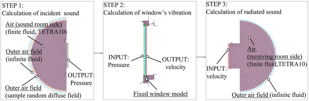
FIGURE 9. Calculation flow of the weak-coupling model.

Regarding the problem size of each step, the total nodes in the numerical model of Step 1 are 377,896 and 750,873, respectively, for window (A) and window (D). For Step 2, the window (A) and (D) models have 240,446 nodes and 497,591 nodes, respectively, which is the same as the baseline model. In Step 3, the total numbers of nodes are 402,635 and 715,370, respectively, for windows (A) and (D). Compared to the strong-coupling model, the maximum problem size is reduced to less than half. This problem size reduction markedly reduces memory consumption, especially for larger windows. However, the two additional analyses of Step 1 and Step 3 entail larger problem sizes than the baseline model. The computations are performed in parallel using four processes.

The SRI is also computed from the incident sound power W_inc computed in Step 1 and sound radiation power W_rad computed in Step 3, with Eq. 10. The element sizes are the same as those for the models used in the strong-coupling model described in an earlier section. It is noteworthy that Step 1 and Step 3 can perform as acoustic analysis.

4.2 Results

Figure 10 shows the SRIs of fixed windows calculated respectively using the weak-coupling model and absolute errors from measurements in the upper and lower panels. The weak-coupling model produced much better accuracy than the baseline model results as shown in Figure 6B at 125 Hz–1 kHz. Greater improvement can be found for smaller windows. It is noteworthy that the weak-coupling model can also reproduce the small dips in SRI at 315 and 800 Hz appeared in the measured results of window (A). The absolute errors in the weak-coupling model are less than 3.3 dB, except for the result of window (A) at 100 Hz. The resulting accuracy is comparable to strong-coupling model results obtained for windows (B)–(E), but slightly lower accuracy to the smallest window (A) can be observed.

FIGURE 10

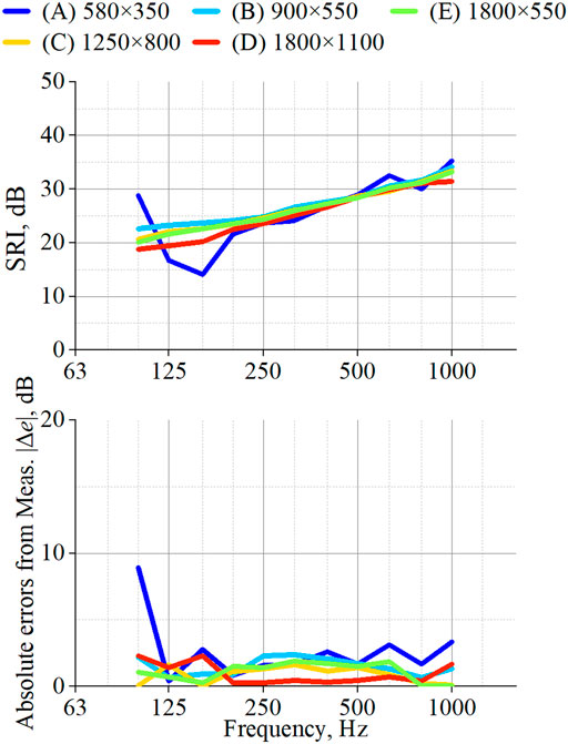
FIGURE 10. Results obtained using the weak-coupling model (Upper) SRIs of five fixed windows and (Bottom) absolute difference from measured SRIs.

Furthermore, as expected, the weak-coupling model has special benefits for maximum memory requirements. For the minimum-sized window (A) and the maximum-sized window (D), the weak-coupling models respectively require 29 and 51 GB per process, which are 1/2.7 and 1/4 less memory than the strong-coupling models. Moreover, the computational times for windows (A) and (D) are 36,288 s and 98,921 s. They are 1.7 and 3.6 times faster, respectively, than the strong-coupling model. The results demonstrate the effectiveness of using the weak-coupling model to compute SRIs in a laboratory environment at a low frequency range.

5 Conclusion

This study explored efficient and accurate finite element modeling to predict SRI of different-sized fixed windows at random incidence in a laboratory environment. To this end, we examined the prediction accuracy of three numerical models over five fixed windows with different dimensions of 0.2–2.0 m² by comparison with measured results. All numerical models incorporate the assumption of a diffused sound-incidence condition. Sound radiated from windows is computed using Rayleigh’s integral or sound field analysis using acoustic analysis. We also examined necessary computational costs for the three numerical models to infer a practical prediction model according to the analyzed frequency range. The findings obtained from our study are presented below.

1) The simplest model that discretizes only window parts with finite elements shows higher accuracy at first normal mode and around and above coincidence frequencies when using measured total loss factors instead of using internal loss factors of the respective materials. The computational costs are practical for computing SRI up to 5 kHz, with the calculation of 1/24 octave band center frequencies. The largest window(D) can be calculated within 8 h using 45 GB per process. However, an important shortcoming of this simplest model is that it can not accurately reproduce SRI in a laboratory environment below coincidence frequencies, especially for smaller windows, because of neglect of the niche in the numerical model.

2) The strong-coupling model with a niche that discretizes the window and surrounding hemisphere sound fields with niche has the best prediction of SRI below 1 kHz in a laboratory environment. A niche must be included in the numerical model for the accurate prediction of SRI in smaller-sized windows. However, the strong-coupling model entails high computational burdens. The strong-coupling model requires 6–7.5 times larger computational memory than the simplest model, even for the analysis below 1 kHz. Therefore, the practical use of the strong-coupling model is difficult for SRI prediction at high frequencies.

3) The weak-coupling model which divides the strong-coupling model calculation into three steps can still produce a comparable accuracy to the strong-coupling model in SRI predictions below 1 kHz, with higher efficiency. The computational cost reduced to 1/2.7–1/4 than the strong coupling model. The SRI of the largest window (D) can calculate within 27 h until 1 kHz. Therefore, using the weak-coupling model is a practical selection to predict SRI at low frequencies when considering niche effects in a laboratory environment.

Data availability statement

The raw data supporting the conclusions of this article will be made available by the authors, without undue reservation.

Author contributions

MM contributed to the conception and design of the study, conducted the experiment and numerical simulations, and prepared the draft of the manuscript. TO and KS contributed to give feedback about the research design and numerical simulations, analyzed the results, and supported writing of the manuscript. All authors contributed to manuscript revision, reading, and approval of the submitted version.

Conflict of interest

Author MM is employed by YKK Corporation.

The remaining authors declare that the research was conducted in the absence of any commercial or financial relationships that could be construed as a potential conflict of interest.

Publisher’s note

All claims expressed in this article are solely those of the authors and do not necessarily represent those of their affiliated organizations, or those of the publisher, the editors and the reviewers. Any product that may be evaluated in this article, or claim that may be made by its manufacturer, is not guaranteed or endorsed by the publisher.

References

Arjunan, A., Wang, C., Yahiaoui, K., Mynors, D., Morgan, T., and English, M. (2013). Finite element acoustic analysis of a steel stud based double-leaf wall. Build. Environ. 67, 202–210. doi:10.1016/j.buildenv.2013.05.021

CrossRef Full Text | Google Scholar

Arjunan, A., Wang, C., Yahiaoui, K., Mynors, D., Morgan, T., Nguyen, V., et al. (2014). Development of a 3d finite element acoustic model to predict the sound reduction index of stud based double-leaf walls. J. Sound Vib. 333, 6140–6155. doi:10.1016/j.jsv.2014.06.032

CrossRef Full Text | Google Scholar

Astley, R. J., and Coyette, J.-P. (2001a). Conditioning of infinite element schemes for wave problems. Commun. Numer. Methods Eng. 17, 31–41. doi:10.1002/1099-0887(200101)17:1¡31::AID-CNM386¿3.0.CO;2-A

CrossRef Full Text | Google Scholar

Astley, R. J., and Coyette, J.-P. (2001b). The performance of spheroidal infinite elements. Int. J. Numer. Methods Eng. 52, 1379–1396. doi:10.1002/nme.260

CrossRef Full Text | Google Scholar

Cambridge, J. E., Davy, J. L., and Pearse, J. (2020). The sound insulation and directivity of the sound radiation from double glazed windows. J. Acoust. Soc. Am. 148, 2173–2181. doi:10.1121/10.0002167

PubMed Abstract | CrossRef Full Text | Google Scholar

Coyette, J.-P., van den Nieuwenhof, B., and Lielens, G. (2014). “Computational strategies for modeling distributed random excitations (diffuse field and turbulent boundary layer ) in a vibro-acoustic context,” in Congres francais d’Acoustique.

Google Scholar

Davy, J. L. (2009). Predicting the sound insulation of single leaf walls: Extension of cremer’s model. J. Acoust. Soc. Am. 126, 1871–1877. doi:10.1121/1.3206582

PubMed Abstract | CrossRef Full Text | Google Scholar

Davy, J. L. (2010). The improvement of a simple theoretical model for the prediction of the sound insulation of double leaf walls. J. Acoust. Soc. Am. 127, 841–849. doi:10.1121/1.3273889

PubMed Abstract | CrossRef Full Text | Google Scholar

Free Field Technologies (2019). Actran 2020 user’s guide–volume 1: Installation, operations, theory and utilities. Mont-Saint-Guibert, Belgium: Free Field Technologies.

Google Scholar

Guy, R., De Mey, A., and Sauer, P. (1985). The effect of some physical parameters upon the laboratory measurements of sound transmission loss. Appl. Acoust. 18, 81–98. doi:10.1016/0003-682X(85)90039-8

CrossRef Full Text | Google Scholar

ISO 10140-1 (2016). Acoustics – laboratory measurement of sound insulation of building elements – Part 1: Application rules for specific products. Geneva: International Organization for Standardization.

Google Scholar

JIS A 1416 (2000). Acoustics-method for laboratory measurement of airborne sound insulation of building elements.

Google Scholar

Kim, B.-K., Kang, H.-J., Kim, J.-S., Kim, H.-S., and Kim, S.-R. (2004). Tunneling effect in sound transmission loss determination: Theoretical approach. J. Acoust. Soc. Am. 115, 2100–2109. doi:10.1121/1.1698815

CrossRef Full Text | Google Scholar

Kirkup, S. (1994). Computational solution of the acoustic field surrounding a baffled panel by the Rayleigh integral method. Appl. Math. Model. 18, 403–407. doi:10.1016/0307-904x(94)90227-5

CrossRef Full Text | Google Scholar

Løvholt, F., Norèn-Cosgriff, K., Madshus, C., and Ellingsen, S. E. (2017). Simulating low frequency sound transmission through walls and windows by a two-way coupled fluid structure interaction model. J. Sound Vib. 396, 203–216. doi:10.1016/j.jsv.2017.02.026

CrossRef Full Text | Google Scholar

Mimura, M., Okuzono, T., and Sakagami, K. (2022a). Pilot study on numerical prediction of sound reduction index of double window system: Comparison of finite element prediction method with measurement. Acoust. Sci. Technol. 43, E2131–E2142. doi:10.1250/ast.43.32

CrossRef Full Text | Google Scholar

Mimura, M., Tsukamoto, Y., Tomikawa, Y., Okuzono, T., and Sakagami, K. (2022b). Sound insulation characteristics of small fixed windows in a laboratory and prediction with an existing theory. Acoust. Sci. Technol. In print.

Google Scholar

Minichilli, F., Gorini, F., Ascari, E., Bianchi, F., Coi, A., Fredianelli, L., et al. (2018). Annoyance judgment and measurements of environmental noise: A focus on Italian secondary schools. Int. J. Environ. Res. Public Health 15, 208. doi:10.3390/ijerph15020208

PubMed Abstract | CrossRef Full Text | Google Scholar

Muzet, A. (2007). Environmental noise, sleep and health. Sleep. Med. Rev. 11, 135–142. doi:10.1016/j.smrv.2006.09.001

PubMed Abstract | CrossRef Full Text | Google Scholar

Papadopoulos, C. I. (2003). Development of an optimised, standard-compliant procedure to calculate sound transmission loss: Numerical measurements. Appl. Acoust. 64, 1069–1085. doi:10.1016/S0003-682X(03)00066-5

CrossRef Full Text | Google Scholar

Petri, D., Licitra, G., Vigotti, M. A., and Fredianelli, L. (2021). Effects of exposure to road, railway, airport and recreational noise on blood pressure and hypertension. Int. J. Environ. Res. Public Health 18, 9145. doi:10.3390/ijerph18179145

PubMed Abstract | CrossRef Full Text | Google Scholar

Petyt, M. (2010). Introduction to finite element vibration analysis. New York: Cambridge University Press.

Google Scholar

Rindel, J. (2018). Sound insulation in buildings. Boca Raton: CRC Press.

Google Scholar

Sakuma, T., Inoue, N., and Seike, T. (2017). Numerical examination of niche effect on sound transmission loss of glass panes. Acoust. Sci. Technol. 38, 279–286. doi:10.1250/ast.38.279

CrossRef Full Text | Google Scholar

Sandberg, G., Wernberg, P.-A., and Davidsson, P. (2008). “Fundamentals of fluid-structure interaction,” in Computational aspects of structural acoustics and vibration (Berlin, Germany: Springer), 23–101.

CrossRef Full Text | Google Scholar

Santoni, A., Davy, J. L., Fausti, P., and Bonfiglio, P. (2020). A review of the different approaches to predict the sound transmission loss of building partitions. Build. Acoust. 27, 253–279. doi:10.1177/1351010X20911599

CrossRef Full Text | Google Scholar

Sewell, E. (1970). Transmission of reverberant sound through a single-leaf partition surrounded by an infinite rigid baffle. J. Sound Vib. 12, 21–32. doi:10.1016/0022-460X(70)90046-5

CrossRef Full Text | Google Scholar

Soussi, C., Aucejo, M., Larbi, W., and Deü, J.-F. (2021). Numerical analyses of the sound transmission at low frequencies of a calibrated domestic wooden window. Proc. Institution Mech. Eng. Part C J. Mech. Eng. Sci. 235, 2637–2650. doi:10.1177/09544062211003621

CrossRef Full Text | Google Scholar

Tsukamoto, Y., Tamai, K., Sakagami, K., Okuzono, T., and Tomikawa, Y. (2021). Basic study of practical prediction of sound insulation performance of single-glazed window. Acoust. Sci. Technol. 42, E2143–E2353. doi:10.1250/ast.42.350

CrossRef Full Text | Google Scholar

Van den Nieuwenhof, B., Lielens, G., and Coyette, J. (2010). “Modeling acoustic diffuse fields: Updated sampling procedure and spatial correlation function eliminating grazing incidences,” in The Proceedings of ISMA Conference, 4723–4736.

Google Scholar

Vinokur, R. (2006). Mechanism and calculation of the niche effect in airborne sound transmission. J. Acoust. Soc. Am. 119, 2211–2219. doi:10.1121/1.2179656

PubMed Abstract | CrossRef Full Text | Google Scholar

Wawezynowicz, A., Krzaczek, M., and Tejchman, J. (2014). Experiments and fe analyses on airborne sound properties of composite structural insulated panels. Archives Acoust. 39, 351–364. doi:10.2478/aoa-2014-0040

CrossRef Full Text | Google Scholar

Wittig, L. E., and Sinha, A. K. (1975). Simulation of multicorrelated random processes using the fft algorithm. J. Acoust. Soc. Am. 58, 630–634. doi:10.1121/1.380702

CrossRef Full Text | Google Scholar