Evaluation of crack propagation in concrete bridges from vehicle-mounted camera images using deep learning and image processing

1 Introduction

In recent years, the structural integrity of social infrastructures, which have become unsafe due to aging, has become a great concern, and how to efficiently and accurately assess their structural integrity is important in developing maintenance plans. In 2015, the Road Act of Japan was revised to require close visual inspections once every 5 years for bridges with spans of 2 m or more. Currently, these bridges are visually inspected by professional engineers. However, in preparation for the shortage of engineers in the future due to the declining population, it is important to develop labor saving system for inspections while ensuring the inspection accuracy of skilled engineers.

In the past few decades, many traditional computer vision technologies, for example, threshold segmentation Cheng et al. (2003); Fujita et al. (2006), Otsu, 1979 (Otsu, 1979), edge detection (Behara et al. (2012); Martin et al. (2004), and seed region growth Huang and Xu, (2006); Li et al. (2011) have been explored in vison-based crack detection. However, the detection accuracy of these methods does not meet the engineering requirements for real applications. Also, as a representative study aiming at labor-saving visual inspection work, a method to create damage maps by detecting and quantifying cracks from images acquired by Unmanned Aerial Vehicles (UAVs) equipped with cameras has been proposed. Nishimura et al. (2012). Have developed a technique for quantifying crack opening width etc. From 3D models constructed by Structure from Motion (SfM) and from a large number of orthoimages through image processing (Nishimura et al., 2012a; Nishimura et al., 2012b). However, since SfM constructs a 3D model using the correlation of luminance distribution among images taken, it is difficult to evaluate the damage including cracks depending on the state of the object surface, such as a structure with uniform luminance distribution due to painting. On the other hand, the recent dramatic improvement in image/pattern recognition accuracy through artificial intelligence and deep learning has led to the development of inspection of social infrastructures. Numerous studies have been conducted on the detection of cracks in concrete for a variety of subjects. Chun and Igo et al. (2015) proposed a method for detecting cracks on concrete surfaces using Random Forest (Chun and Igo, 2015). Random Forest is an algorithm that performs classification according the results of multiple decision trees constructed from randomly selected training data and explanatory variables. Yoshida et al. (2020) proposed a method to detect crack initiation points using a deep learning model from panoramic images of riverbank revetments and to evaluate the actual size of crack detection from orthoimages (Yoshida et al., 2020). However, this method has been applied to only one type of design, and it has been shown that the accuracy of crack detection is greatly reduced for different structures. The uniformity of the structural part of the riverbank revetment also makes it easier for the learning model to recognize the feature patterns in the crack region. Cha et al. (2017) constructed a convolutional neural network that performs two-class classification: “cracked” and “intact” (Cha et al., 2017). The results show that cracks are detected with higher accuracy than the traditional Canny and Sobel edge detection methods Canny, (1986), Kanopoulos et al. (1988). Dung and Anh (2108) proposed an encoder-decoder FCN for segmenting an image of concrete crack into “crack” and “non-crack” pixels (Dung and Anh, 2018). Their proposed architecture was trained end-to-end on a subset of crack images of the same dataset and reached approximately 90% for both the max F1 and AP scores on training, validation, and test sets. However, the system is shown to be susceptible to ambient noise. Ju et al. (2019) developed a crack deep network based on the Faster Region Convolutional Neural Network (Fast-RCNN) (Ju et al., 2019). Results indicated that the developed system achieves the detection mean average precision of higher than 0.90, which outperforms both the original Faster-RCNN and SSD300, but requires intense computational resources. Liu et al. (2019) used U-Net network structure to build a deep learning model for crack detection (Liu et al., 2019). The proposed system was found to be accurate detections, but only accepts 3 × 512 × 512 image input. There is still a long way to go for engineering applications. Also, in recent years, pixel-level crack detection systems have been proposed. Bang et al. (2019) proposed a pixel-level crack detection system based on a deep convolutional encoder-detector network (Bang et al., 2019). Liu et al. (2020) proposed a two-step pavement crack detection and segmentation method based on CNN where the modified YOLOv3 (Redmon and Farhadi, 2018) and U-Net (Ronneberger et al., 2015) were, respectively, used for these two tasks. The results indicated that the precision, recall, and F1 score of proposed pavement crack detection and segmentation system are higher than other state-of the-art methods. Yamane et al. (2019) proposed a pixel-level crack detection method using Convolutional Neural Networks (CNN) and Mask R-CNN (He et al., 2018) which is one of semantic segmentation techniques. Meanwhile, numerous studies have been also conducted on damage detection in steel structures. Konovalenko et al. (2021) developed a classification system based on residual neural network for damage of metal surfaces such as scratches, scrapes and abrasions (Konovalenko et al., 2021). The results shows that the best model classifier is based on ResNet152 deep convolutional neural network. As for pixel-level defect detection for metal surfaces, Konovalenko et al. (2022) developed and researched 14 neural network models (Konovalenko et al., 2022). U-Net-like architectures with encoders such as ResNet (He et al., 2015), DenseNet (Huang et al., 2018) and so on were investigated as part of the problem, which consisted in detecting defects such as “scratch abrasion”. Results show that the highest recognition accuracy was attained using the U-Net model with a ResNet152 backbone. Most of the above-mentioned studies have been successful in detecting cracks or some kind of defects with high accuracy; however, they do not describe the aging or propagation of damage. In addition, Deep learning and Machine Learning based image classification systems, which have been applied in the above studies, require more time to detect damage in a single image than detection system because it is necessary to determine whether a crack is present or not. These are time-consuming processes when inspecting large structures, so there is room for improvement in terms of time efficiency. Moreover, deep learning methods require the generation of a large amount of data because accuracy is affected by the training data, which is a challenge in terms of labor-saving training data generation.

In this study, we attempt to develop a system that can detect damage on structural surfaces with high accuracy and high speed, and also a system that automatically outputs not only the damage initiation area but also progression area, by utilizing the visual inspection results accumulated by engineers. We also attempt to semi-automatically convert the accumulated visual inspection results into YOLO training data in order to save labor in the creation of training data. The proposed system is a multi-stage system that applies object recognition technology using convolutional neural networks (CNN) and a morphology algorithm that detects damage in pixel units based on the characteristics of image brightness values, in addition to detection technology using YOLO, which can detect objects in moving images. To illustrate the applicability of the method developed here, some experiments are conducted by using the photos of running surface of concrete bridges of a monorail took by vehicle-mounted camera.

2 System flowchart

This study uses images taken from an on-board camera to inspect the concrete surface of a 40-km monorail bridge, the running surface. The main types of damage are cracks and free lime. The training data is created based on the images of inspection results that have been accumulated by the administrator. The system proposed in this study can be divided into five stages of processing. The first stage of processing uses YOLOv2 (Redmon and Farhadi, 2016), a common object detection algorithm, to detect damaged areas. The data applied in this study deals with a large set of images, which is about 100,000 images. Therefore, it is appropriate to use YOLOv2 for damage detection because of its high detection speed. The images handled in the second and subsequent stages are more limited than those detected in the first stage, and this data limitation can significantly reduce processing time. In the second stage of processing, the area where damage was detected by YOLOv2 is first trimmed. Next, images of the damaged area are collected, and the damaged area is carefully inspected using the network model VGG16 (Simonyan and Zisserman, 2015), because damage detection by YOLOv2 alone may result in over-detection. The third stage of processing uses a morphological algorithm to extract pixel-by-pixel cracks from the damage area examined in the second stage of processing. Pixel-by-pixel damage detection allows for more accurate application to the fifth step, progression evaluation processing. Morphological image processing includes color correction, median filtering, line enhancement, and binarization. After morphological processing, the areas of damage are colored with a specified color. In the fourth stage of processing, the binarized damage areas are attached to the original image. This makes it possible for the inspection engineer to identify the location of damage in the original image. In the final stage of processing, the difference in the damaged area is extracted as an evaluation of the progress of damage. Here, the evaluation of the progress is carried out through the comparison with images evaluated in the above processing at the time of the previous inspection is used.

3 Damage detection based on deep learning

3.1 You only look once

The screening technique for structural surface damage in this study is based on general object detection using deep learning, and YOLO (Redmon et al., 2016) is used as a detection technique. The main feature of YOLO for object detection is that it simultaneously extracts a candidate region of a target object and calculates the class probability of that candidate region in a single guess. This makes it possible to perform object detection at very high speed and in real time, even for moving images. YOLO is one of the fastest general object detection systems proposed so far, but the same authors have also proposed YOLOv2 and YOLOv3, which enable object detection with higher accuracy. They, like YOLO, are provided as part of Darknet. In this study, we use YOLOv2, which is the fastest detection method. The inference flow of the YOLO system is shown below.

3.2 Inference procedure

Figure 1 shows the inference procedure for YOLO. The first step is to divide the input image into S × S grid cells. Each grid cell has several bounding boxes, as shown in Figure 2, and the confidence for each box is calculated. Confidence is calculated as follows.

$\mathit{C}\mathit{o}\mathit{n}\mathit{f}\mathit{i}\mathit{d}\mathit{e}\mathit{n}\mathit{c}\mathit{e}=\mathit{Pr}\left(\mathit{O}\mathit{b}\mathit{j}\mathit{e}\mathit{c}\mathit{t}\right)\bullet {\mathit{I}\mathit{O}\mathit{U}}_{\mathit{p}\mathit{r}\mathit{e}\mathit{d}}^{\mathit{t}\mathit{r}\mathit{u}\mathit{t}\mathit{h}}$

${\mathit{I}\mathit{O}\mathit{U}}_{\mathit{p}\mathit{r}\mathit{e}\mathit{d}}^{\mathit{t}\mathit{r}\mathit{u}\mathit{t}\mathit{h}}=\left|\frac{{\mathit{B}}_{\mathit{i}}\cap \mathit{g}\mathit{r}\mathit{o}\mathit{u}\mathit{n}\mathit{d}\_\mathit{t}\mathit{r}\mathit{u}\mathit{t}\mathit{h}}{{\mathit{B}}_{\mathit{i}}\cup \mathit{g}\mathit{r}\mathit{o}\mathit{u}\mathit{n}\mathit{d}\_\mathit{t}\mathit{r}\mathit{u}\mathit{t}\mathit{h}}\right|$

where Pr(Object) is the probability that the bounding box contains some object, and ${\mathit{I}\mathit{O}\mathit{U}}_{\mathit{p}\mathit{r}\mathit{e}\mathit{d}}^{\mathit{t}\mathit{r}\mathit{u}\mathit{t}\mathit{h}}$ (Intersection Over Union) is the proportion of overlap between the bounding box (B_i) predicted from the grid cells and the object (ground_truth) in the image actually given as training data, which is shown in Figure 3. The confidence level is composed of the product of the probability Pr(Object) that a bounding box contains an object and the overlap ratio IOU between the bounding box and the ground truth. If there is no object to be detected in the grid cell of interest, then each bounding box has a confidence level of 0, since there is no object in that box. In addition to the confidence level, each bounding box keeps its own center coordinates (x, y) and size (height, width) as predicted in YOLO.

FIGURE 1

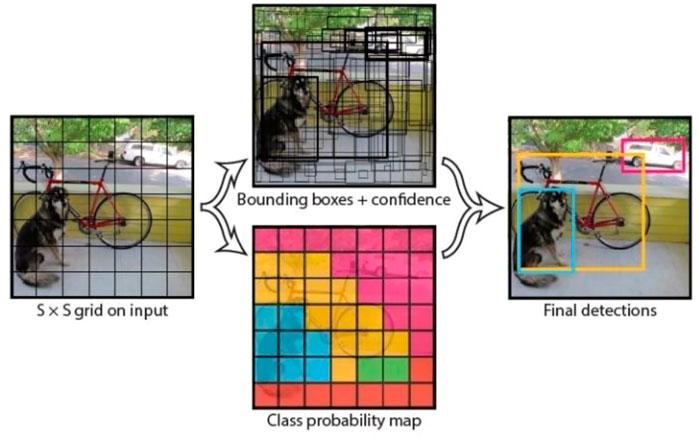
FIGURE 1. Object detection by YOLO (Redmon et al., 2016).

FIGURE 2

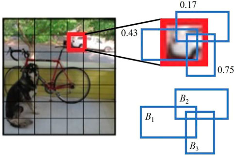
FIGURE 2. Bounding box and Confidence.

FIGURE 3

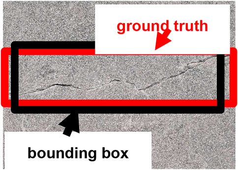
FIGURE 3. Ground_truth and bounding box in IOU.

On the other hand, a grid cell has a conditional class probability Pr(Class_i | Object) whether the object to be detected is contained within its own grid cell or not. For example, the grid cell of interest in Figure 1 has Pr(Class = Dog | Object) = 0.05, Pr(Class = Car | Object) = 0.92, Pr(Class = Bicycle | Object) = 0.03, etc. Then, each grid cell outputs two bounding boxes with high confidence, which are expressed in terms of thickness as the bounding box + confidence in Figure 1, depending on the magnitude of the confidence. Finally, only the bounding boxes with confidence exceeding the threshold are adopted, and the class of the bounding box is determined by combining the adopted bounding box and the class with the highest probability in the corresponding grid cell (final detection in Figure 1). As described above, YOLO’s general object detection is structured in such a way that class classification is performed for each grid cell region and the bounding box is used to detect candidate object regions. YOLO randomly generates three bounding boxes with a certain aspect ratio in each grid cell.

3.3 How to learn you only look once

YOLO is trained with a convolutional neural network consisting of convolutional layers (conv. layers) and all connected layers (conn. layers), although the number of layers varies with each version. YOLO outputs the location information (x, y, height, width) and confidence level of the two bounding boxes and the category to be detected for each grid cell in the input image. Therefore, the number of units in the output layer is the sum of the number of classes to be detected, the location information of the two bounding boxes, and the confidence level [(x, y, height, width, confidence level) × 2], multiplied by the number of grids S × S. The loss functions for optimizing the filters and biases in the network are shown below.

$\mathbf{L}\mathbf{o}\mathbf{s}\mathbf{s}\mathbf{f}\mathbf{u}\mathbf{n}\mathbf{c}\mathbf{t}\mathbf{i}\mathbf{o}\mathbf{n}={\mathit{\lambda }}_{\mathbf{c}\mathbf{o}\mathbf{o}\mathbf{d}}{\sum }_{\mathit{i}=\mathbf{0}}^{{\mathit{S}}^{\mathbf{2}}}{\sum }_{\mathit{j}=\mathbf{0}}^{\mathit{B}}{\mathit{I}}_{\mathit{i}\mathit{j}}^{\mathbf{o}\mathbf{b}\mathbf{j}}\left[{\left({\mathit{x}}_{\mathit{i}}-{\widehat{\mathit{x}}}_{\mathit{i}}\right)}^{\mathbf{2}}+{\left({\mathit{y}}_{\mathit{i}}-{\widehat{\mathit{y}}}_{\mathit{i}}\right)}^{\mathbf{2}}\right]{+\mathit{\lambda }}_{\mathbf{c}\mathbf{o}\mathbf{o}\mathbf{d}}{\sum }_{\mathit{i}=\mathbf{0}}^{{\mathit{S}}^{\mathbf{2}}}{\sum }_{\mathit{j}=\mathbf{0}}^{\mathit{B}}{\mathit{I}}_{\mathit{i}\mathit{j}}^{\mathbf{o}\mathbf{b}\mathbf{j}}\left[{\left(\sqrt{{\mathit{w}}_{\mathit{i}}}-\sqrt{{\widehat{\mathit{w}}}_{\mathit{i}}}\right)}^{\mathbf{2}}+{\left(\sqrt{{\mathit{h}}_{\mathit{i}}}-\sqrt{{\widehat{\mathit{h}}}_{\mathit{i}}}\right)}^{\mathbf{2}}\right]+{\sum }_{\mathit{i}=\mathbf{0}}^{{\mathit{S}}^{\mathbf{2}}}{\sum }_{\mathit{j}=\mathbf{0}}^{\mathit{B}}{\mathit{I}}_{\mathit{i}\mathit{j}}^{\mathit{o}\mathit{b}\mathit{j}}{\left({\mathit{C}}_{\mathit{i}}-{\widehat{\mathit{c}}}_{\mathit{i}}\right)}^{\mathbf{2}}+{\mathit{\lambda }}_{\mathbf{n}\mathbf{o}\mathbf{o}\mathbf{b}\mathbf{j}}{\sum }_{\mathit{i}=\mathbf{0}}^{{\mathit{S}}^{\mathbf{2}}}{\sum }_{\mathit{j}=\mathbf{0}}^{\mathit{B}}{\mathit{I}}_{\mathit{i}\mathit{j}}^{\mathbf{n}\mathbf{o}\mathbf{o}\mathbf{b}\mathbf{j}}{\left({\mathit{C}}_{\mathit{i}}-{\widehat{\mathit{c}}}_{\mathit{i}}\right)}^{\mathbf{2}}+{\sum }_{\mathit{i}=\mathbf{0}}^{{\mathit{S}}^{\mathbf{2}}}{\mathit{I}}_{\mathit{i}}^{\mathbf{o}\mathbf{b}\mathbf{j}}{\sum }_{\mathit{c}\in \mathbf{c}\mathbf{l}\mathbf{a}\mathbf{s}\mathbf{s}\mathbf{e}\mathbf{s}}{\left({\mathit{p}}_{\mathit{i}}\left(\mathit{c}\right)-{\widehat{\mathit{p}}}_{\mathit{i}}\left(\mathit{c}\right)\right)}^{\mathbf{2}}$

where$I_{ij}^{\mathrm{o}\mathrm{b}\mathrm{j}}$ is a function that returns 1 if the center coordinate of the j-th bounding box is in the i-th grid cell and 0 otherwise, and$I_i^{\mathrm{o}\mathrm{b}\mathrm{j}}$ returns 1 if the object is in grid cell i and 0 otherwise. Note that${\lambda }_{\mathrm{c}\mathrm{o}\mathrm{o}\mathrm{d}}$ and${\lambda }_{\mathrm{n}\mathrm{o}\mathrm{o}\mathrm{b}\mathrm{j}}$ are the program’s default settings of 5 and 0.5, respectively, but these values can be set arbitrarily. In this study, the default settings are used. The first term of the loss function is the sum of the predicted center coordinates of the bounding box (${\widehat{x}}_i,{\widehat{y}}_i$ ) and the center coordinates of the object’s cutout region (ground_truth) given as the training data ($x_i,y_i$ ) of the object’s cutout region (ground_truth) given as the training data. The second term represents the error between the predicted size of the bounding box (height, weight) = (${\widehat{h}}_i,{\widehat{w}}_i$ ) and the size of the object’s cutout area (ground_truth) given in the training data (height, weight) = ($h_i,w_i$ ) of the object given in the training data. The third term corresponds to the confidence level of the bounding box${\widehat{c}}_i$ and the confidence level of the training data$C_i$ (=1), which is calculated only for the grid cell with the center coordinates of the bounding box. The fourth term computes the prediction error of the unreliability of the bounding box, and is computed only for grid cells that do not have the center coordinates of the bounding box. The fifth term computes the error in the conditional class probability${\widehat{p}}_i\left(c\right)$ for the classification of a grid cell. The filters and biases inside the deep convolutional neural network are optimized so that each of the above five terms converges to zero.

3.4 Learning of supervisory data from crack images

When performing general object detection, training data requires a region cut out from the image data of the object to be detected, the location information such as the center coordinates and size of the region, and a labeled class. YOLO reads the location information of the object to be detected and automatically generates training data. The network weight coefficients are learned using the image of the object and the object’s location. Image processing software is used to extract the image data and positional information from the image data, but LabelImg is used in this study. This method prepares an image showing cracks, specifies the cracked area from the image, and creates location information for YOLOv2 objects. Figure 4 shows an example of cutting out an object from an image. In this study, 25,000 images of cracks were prepared, from which the objects to be detected were extracted in detail and reserved as training data (ground_truth). The rectangular region in each image serves as the ground_truth during training. However, YOLOv2 performs random resizing, mirror image flipping, rotation, and HSV color space transformation on the teacher images during training to increase the number of apparently different image types (data augmentation). The convolutional neural network in this study uses the weights of a trained network for general object detection provided by the YOLOv2 developers as initial values. In one epoch, 64 images and their associated ground_truth were randomly selected for training, and training was completed in 100,000 epochs. The average IOU at the end of training was about 0.8. Considering our previous experience and the reliability of the objects, we judged that the given training data were adequately trained.

FIGURE 4

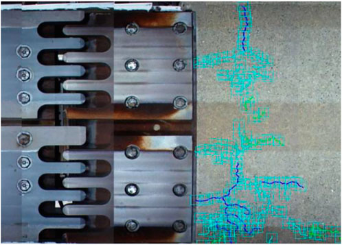
FIGURE 4. An example of annotation data.

3.5 Detection result

Figure 5 shows an example of detection results. In Figure 5, the crack tracing results, which were visually confirmed by the engineer, are overlaid to make the detection results easier to understand. As shown in Figure 5, although some over-detection was observed, the recall of 50 images with cracks was about 88.9%. The recall in this study was calculated as the ratio of the total number of pixels of cracks traced by the engineer to the number of traced pixels in the predicted rectangular area.

FIGURE 5

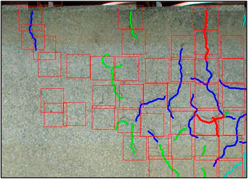
FIGURE 5. An example of detection results.

4 Post-detection scrutiny by convolutional neural networks-based image recognition

In object detection using YOLOv2, increasing the confidence threshold for crack and other class classification results enables detection of only highly accurate areas, but it is likely to increase the lack of detection of small cracks. On the other hand, lowering the threshold reduces the number of the lack of detection of small cracks, but at the same time, dirt on the concrete surface may also be detected as cracks, resulting in more false detections. Therefore, we attempt to improve accuracy by incorporating image recognition technology using CNN after detection, and by conducting a close inspection after crack detection. Specifically, the threshold for the confidence value, which is output from YOLO, is set low, and all the rectangle determined to be a crack in YOLO is cropped as an image. All of the images are then input to the CNN and examined to determine if they are indeed cracks. The images that are not cracks are rejected, and only the images that are cracks are reflected. As described above, the system is designed to reduce both detection omissions and false positives by performing a close inspection using image recognition after detection at a low threshold value. In this study, the CNN used for the scrutiny was a fine-tuned version of VGG16 as a general-purpose model.

VGG16 is a CNN model consisting of 16 layers trained on a large image dataset called ImageNet, and was developed by a research group called VGG at the University of Oxford in 2014. Because of its simple architecture, it is one of the learned models used in various studies. VGG16 consists of 13 convolutional layers and 3 all-connected layers, for a total of 16 layers, and its output layer is a neural network with 1,000 units and 1,000 classes to classify. The structure of the VGG16 model is shown in Figure 6. One of the features of this neural network is that it uses a 3 × 3 convolutional filter, which suppresses the increase in the number of parameters in the deeper layers and improves accuracy. The convolutional stride is fixed at 1 pixel, and there are 5 Maxpooling layers, where the size is halved. The stack of convolutional layers is followed by three all-combining layers. The last layer is the softmax layer, which uses ReLU as the activation function. When utilizing a trained network, feature extraction is processed in the convolutional layer within the network. When new data is applied to the network, a unique classifier is used in the network after the convolutional layer. The convolutional layers can be reused because their feature maps are generic and are likely to be useful in any computer vision application. Based on the results of the aforementioned damage detection, we further classified the data into six different classes.

FIGURE 6

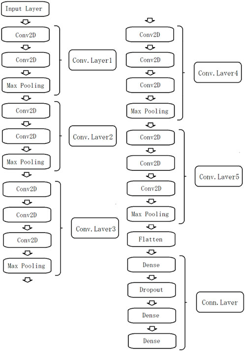
FIGURE 6. Structure of vgg16.

The six classes and the number of images for each class are listed in Table 1. The examples of images in the above six classes are shown in Figure 7. The most important classes are “crack” and “free lime”. Therefore, images identified as “crack” or “free lime” are binarized through morphological processing. In this study, we set a function to terminate learning, which is called as early stopping, to avoid an overlearning. In addition, we employ the Cost-sensitive Learning approach, which defines a loss function that imposes a heavier penalty for misclassification of data with fewer labels due to the unbalanced amount of training data.

TABLE 1

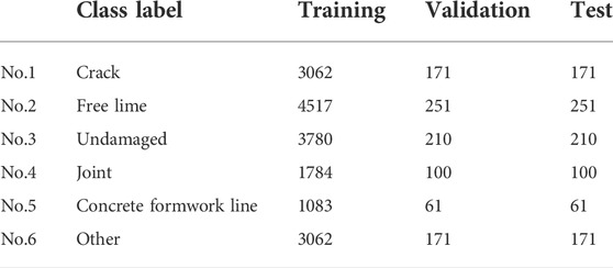
TABLE 1. Classified targets and Number of images.

FIGURE 7

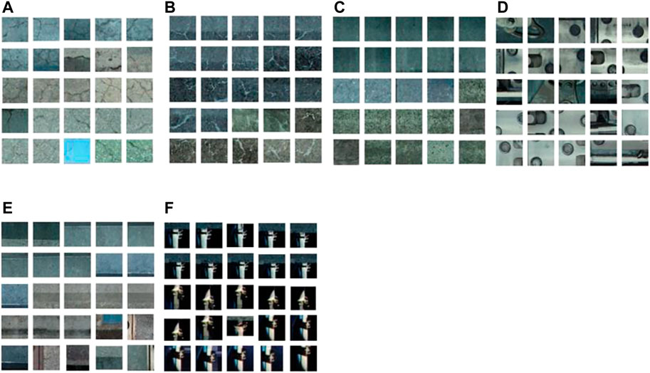
FIGURE 7. An example of Classified targets. (A) Crack. (B) Free lime. (C) Undamaged. (D) Joint. (E) Concrete formwork line. (F) Others.

The time history of errors in the training and validation data is shown in Figure 8. As shown in Table 1, approximately 5% of the data in each class was allocated to the test data. The Precision, Recall, and F1Score for each class is shown in Table 2. It is found from the figure that the F1score is higher than 0.95 for the six classes.

FIGURE 8

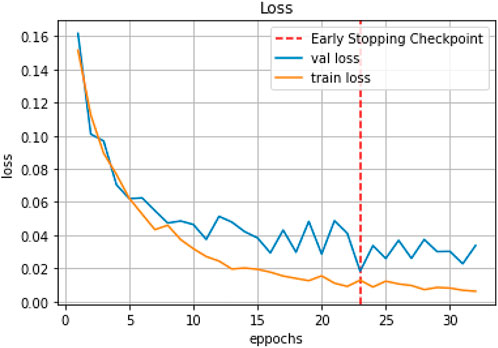
FIGURE 8. Time history of Loss values between training data and validation data.

TABLE 2

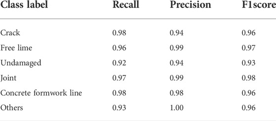
TABLE 2. Classification results for each class.

5 Morphological processing for pixel-by-pixel damage detection

5.1 Color tone correction

In this study, morphological processing is used to enhance linear features from the image luminance value and to binarize cracks and free lime areas. In order to perform damage detection on a pixel-by-pixel basis, a color tone correction process is required as a preprocessing step. The color correction process in this study includes histogram flattening, gamma correction, and contrast correction.

First, histogram flattening reduces variations in the brightness and darkness of the image caused by factors such as illumination placement, shadows, and characteristics of the visible-light camera. Since the histogram flattening process corrects luminance values, it is necessary to correct the exposure level. In this study, gamma correction is used to correct the exposure. Gamma correction results in a luminance value close to black (0) for “cracks” and close to white (255) for “free lime”. Contrast correction is then used to correct for differences in brightness and darkness in the image. In this study, the “cracks” are corrected to be darker than the background, and the “free lime” is corrected to be whiter than the background to emphasize the distinction between the target area and the background area. Figures 9, 10 show examples of images before and after color correction, respectively.

FIGURE 9

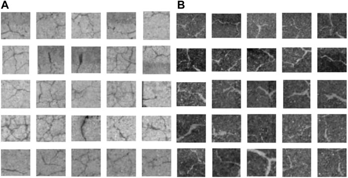
FIGURE 9. Images before color tone correction. (A) Crack. (B) Free lime.

FIGURE 10

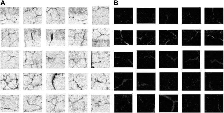
FIGURE 10. Images after color tone correction. (A) Crack. (B) Free lime.

5.2 Median filtering, line enhancement and binarization processing

Contamination is apparent on concrete surfaces. In this study, a median filter is applied to remove elements other than “cracks” and “free lime. The median filter removes spike noise and produces a smoothed image that preserves smooth edges by giving the median value in the local area set by the filter size. Scale line enhancement is then applied to emphasize areas of “cracks” and “free lime”. In this study, the Hesse matrix is applied to the line enhancement process. However, the output value of the line enhancement process has a brightness value of 0 ≤ x ≤ 255 at each pixel. In order to evaluate the progress of damage, it is easier to evaluate the damage concisely if the luminance value at each pixel is 0 or 1. Therefore, in this study, the Canny edge detection algorithm of OpenCV is used to perform binarization detection on the output of the line enhancement process. Figure 11shows examples of the results by binarization for crack and free lime.

FIGURE 11

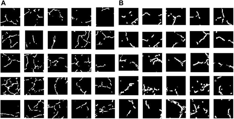
FIGURE 11. Results of binarization. (A) Crack. (B) Free lime.

6 Experiment of damage detection for monorail bridge

In the proposed system, the engineer simply inputs an image and the system performs damage detection using YOLO, damage scrutiny using VGG16 for the detection results by YOLO, and pixel-by-pixel damage detection using binarization based on morphology processing. In other words, the engineer simply inputs an image to the proposed system, and the system outputs the image with the damaged areas colored.

Figures 12, 13 shows an example of the detection results by the proposed system to an image of a concrete girder of a monorail bridge. Green-colored areas indicate free lime, and red-colored areas indicate cracks. Figure 12 shows the detection results for the concrete surface where cracks are dominant as damage (surface A), and Figure 13 shows the detection results for the concrete surface where free lime is dominant as damage (surface B).

FIGURE 12

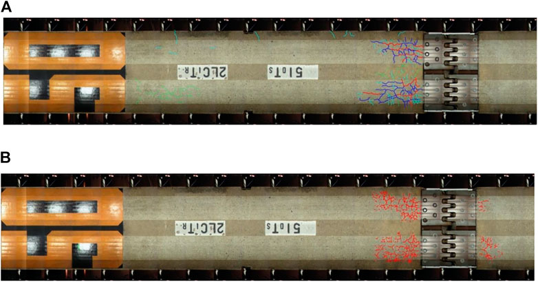
FIGURE 12. An example of the results for concrete girder of monorail bridge (surface A). (A) Damage detection results of manual tracing by engineers. (B) Damage detection results by the proposed system.

FIGURE 13

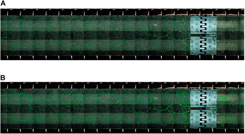
FIGURE 13. An example of the results for concrete girder of monorail bridge (surface B). (A) Damage detection results of manual tracing by engineers. (B) Damage detection results by the proposed system.

Figures 12, 13A are the damage detection results of manual tracing by engineers. Figures 12, 13B are the damage detection results by the proposed system. To quantify the detection accuracy, we evaluated the accuracy of the trace image and the detection result image in pixel units. The evaluation indices of detection accuracy applied in this study were Recall and Precision. Recall was defined as the probability of correctly predicting the correct pixel, and Precision as the probability of being the correct pixel among the predicted pixels. Table 3 shows the performance of damage detection for the surface A and surface B.

TABLE 3

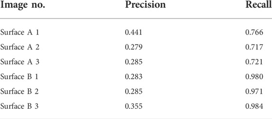
TABLE 3. The performance of damage detection.

As for the surface A, it is shown that Recall obtained a value exceeding 0.7. Meanwhile, as for the surface B, it is found that Recall obtained a value exceeding 0.9. These indicate that although there are some missing detections, the performance of the proposed system is adequate.

In particular, the reason for the high accuracy of the detection of free lime may be that “free lime” has thick line features due to the overflow of white substances such as efflorescence, and the brightness values were easy to distinguish from the those of background of the concrete surface.

On the other hand, Precision is lower than Recall, which indicates that there are many false positives. Thus, further improvement of the system is needed in the future. In addition, it is necessary for engineers to examine the tracing results more closely.

7 Damage progression assessment

In this study, the evaluation of the damage progression is limited to cases where the pixel gap between the two images is within approximately 20px, and is not applicable to cases where the difference between the two images is larger than 20px. In order to evaluate the progress of damage, it is essential to have yearly images taken at the same location. These images are obtained by applying a vehicle-mounted surveying system that continuously acquires three-dimensional coordinate data and visible light images of the road surface. We propose a method to evaluate the progress of the system by allowing for the occurrence of such misalignments.

Specifically, the latest inspection result (Image A) and the inspection result from one period ago (Image B) are prepared, and the damage result is examined pixel by pixel between the two images. The coordinate information (x, y) of damage X in image A is extracted, and the existence of damage X′ corresponding to the coordinate information (x, y) in image B is confirmed; if there is no discrepancy of 1px and the damage occurrence area X and X′ are identical, it is judged that there is no progress and colored white.

However, since the two images usually have a discrepancy in the angle of view, we attempt to check whether the damage exists within the coordinate information (x±α, y±α) in image B. Table 4 shows the range of α and the coloring. If X′ is found in the range of 0≨α ≤ 3, it is colored blue, if X′ is found in the range of 3≨α ≤ 5, it is colored cyan, if X′ is found in the range of 5≨α ≤ 10, it is colored green, if X′ is found in the range of 10 If X′ is found in the range of 5≨α ≤ 5, it is colored green, and if X′ is found in the range of 10≨α ≤ 20, it is colored yellow. If no damage X′ is found in image B after 20px of circumference, it is considered highly likely to be a new damage and is colored red.

TABLE 4

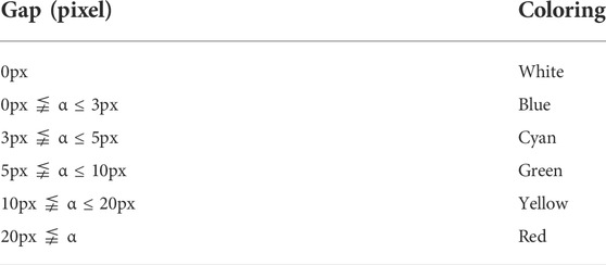
TABLE 4. The range of α and coloring.

Figure 14 shows an example of the evolution of damages such as cracks and free limes in comparison with previous years. In particular, as progress from 2014 to 2015 shown in Figure 14A, while there is overlapping damages between previous years that is visualized in white, there are many areas colored in red. Although this might be due to a discrepancy in the angle of view, it is highly likely that minor cracks and free lime that existed in previous years have developed. On the other hand, as progress from 2015 to 2016 shown in Figure 14B, although red-colored areas are observed, they are fewer than those in Figure 14A. Although this is a qualitative assessment, it suggests that there was not much progression of cracks and free limes between 2015 and 2016.

FIGURE 14

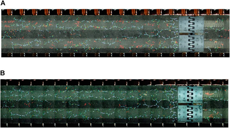
FIGURE 14. An example of Damage progression results. (A) Damage progression in running surface from 2014 to 2015. (B) Damage progression in running surface from 2015 to 2016.

Finally, examples of the details of crack and free-lime progression results are shown in Figures 15, 16, respectively. The left and center figures in Figures 15, 16 show the concrete surface of an area in 2015 and 2016, respectively, while the right figure shows the progression results using the proposed method. As shown in these figures, although it might be not always possible to detect only the areas of progression of damages due to the slip of the both images, the red-colored areas can be identified as newly formed cracks or free limes.

FIGURE 15

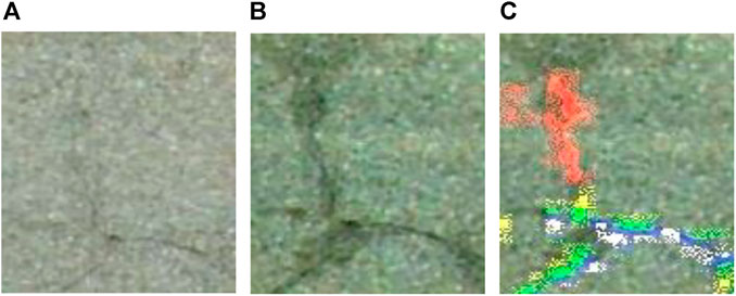
FIGURE 15. The detail of crack progression results. (A) Surface in 2015. (B) Surface in 2016. (C) Progression results of cracks.

FIGURE 16

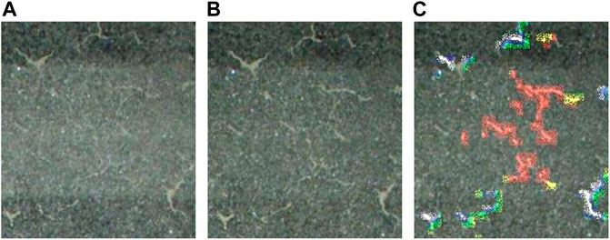
FIGURE 16. The detail of free lime progression results. (A) Surface in 2015. (B) Surface in 2016. (C) Progression results of free limes.

8 Conclusion

The objective of this study was to develop a system that can detect damage on structural surfaces with high accuracy and speed using the results of visual damage inspections, as well as a system that automatically outputs an evaluation of the progress of damage. In addition to the detection technology using YOLO, which is capable of high-speed processing of a large area and a large number of images, we aimed to improve the accuracy of damage detection by using image recognition technology based on CNN and the network model VGG16 to classify the detected rectangular images and introduce scrutiny to the object detection technology. In order to perform the evaluation of progression at the fine pixel level, morphology processing was applied, which is less dependent on the reliability of the trace image as a teacher image compared to deep learning methods. The morphology processing included color correction, median filtering, line enhancement, and binarization, and the final image was output as a pixel-by-pixel damage detection result attached to the original image. By automating these processes, we were able to realize a function in which an engineer inputs the original image and automatically outputs an image in which the damage occurrence areas and the damage development result are drawn on the original image. The findings obtained through this research and future works are summarized as follows.

YOLO was found to be able to detect difficult-to-see damage in images. The results also show that introducing image recognition processing learned by CNN after YOLO detection can improve the accuracy of YOLO. This shows the usefulness of CNNs in terms of performing a close inspection after general object detection.

Through morphological processing, it was found that the recall of damage detection at the pixel level was found to be 0.7 to 0.9.

In the evaluation of progression, a few pixel discrepancies were allowed in stages, and it was possible to identify the areas where progression was likely to be high for minor cracks and free lime that had existed in previous years by coloring the areas in stages.

In the future, the results of inspections by managers, which have been accumulated as training data for object detection and image classification, will be carefully examined, and the latest algorithms, including YOLOv5, which is fast and accurate, will be applied for practical use. In addition, we will attempt to detect cracks and free lime at the pixel level by using deep learning segmentation techniques for binarization of damage. Finally, the proposed method still has many cases of over-detection, so we need to examine the training data again to improve not only the recall but also the precision and so on. We also need to consider image registration techniques for evaluating progress of the crack, since large image shifts can cause problems.

Data availability statement

The original contributions presented in the study are included in the article/supplementary material, further inquiries can be directed to the corresponding author.

Author contributions

All authors listed have made a substantial, direct, and intellectual contribution to the work and approved it for publication.

Conflict of interest

The authors declare that the research was conducted in the absence of any commercial or financial relationships that could be construed as a potential conflict of interest.

Publisher’s note

All claims expressed in this article are solely those of the authors and do not necessarily represent those of their affiliated organizations, or those of the publisher, the editors and the reviewers. Any product that may be evaluated in this article, or claim that may be made by its manufacturer, is not guaranteed or endorsed by the publisher.

References

Bang, S., Park, S., Kim, H. H., and Kim, H. (2019). Encoder-decoder network for pixel-level road crack detection in black-box images. Computer-Aided Civ. Infrastructure Eng. 34 (8), 713–727. doi:10.1111/mice.12440

CrossRef Full Text | Google Scholar

Behara, S., Mohanty, M. N., and Patnaik, S. (2012). “A comparative analysis on edge detection of colloid cyst: A medical imaging approach,” in Soft computing techniques in vision science. Editors P. Srikanta, and Y.-M. Yang (Berlin, Heidelberg: Springer), 63–85.

Google Scholar

Canny, J. (1986). A computational approach to edge detection. IEEE Trans. Pattern Anal. Mach. Intell. PAMI-8, 679–698. doi:10.1109/tpami.1986.4767851

PubMed Abstract | CrossRef Full Text | Google Scholar

Cha, Y.-J., Chai, W., and Büyüköztürk, W. O. (2017). Deep learning-based crack damage detection using convolutional neural networks. Computer-Aided Civ. Infrastructure Eng. 32 (5), 361–378. doi:10.1111/mice.12263

CrossRef Full Text | Google Scholar

Cheng, H. D., Glazier, X. J. C., and Glazier, C. (2003). Real-time image thresholding based on sample space reduction and interpolation approach. J. Comput. Civ. Eng. 17 (4), 264–272. doi:10.1061/(asce)0887-3801(2003)17:4(264)

CrossRef Full Text | Google Scholar

Chun, P., and Igo, A. (2015). Crack detection from image using random forest. J. JSCE 71 (2), I_1–I_8. doi:10.2208/jscejcei.71.i_1

CrossRef Full Text | Google Scholar

Dung, C. V., and Anh, L. D. (2018). Autonomous concrete crack detection using deep fully convolutional neural network. Automation Constr. 99, 52–58.

Google Scholar

Fujita, Y., Mitani, Y., and Hashimoto, Y. (2006). “A method for crack detection on a concrete structure,” in 18^th International conference on pattern recognition (ICPR’06) (IEEE), 3, 901–904. doi:10.1109/icpr.2006.98

CrossRef Full Text | Google Scholar

He, K., Gkioxari, G., Dollar, P., and Girshick, R. (2018). Mask R-CNN. arXiv:1703.06870v3.

Google Scholar

He, K., Zhang, X., Ren, S., and Sun, J. Deep residual learning for image recognition, arXiv:1512.03385v1, (2015).

Google Scholar

Huang, G., Liu, Z., Maaten, L., and Weinberger, K. Q. (2018). Densely counnected convolutional networks. arXiv:1608.06993v5.

Google Scholar

Huang, Y., and Xu, B. (2006). Automatic inspection of pavement cracking distress. J. Electron. Imaging 15 (1), 013017. doi:10.1117/1.2177650

CrossRef Full Text | Google Scholar

Ju, H., Li, W., Tighe, S., Zhai, J., and Chen, Y. (2019). Detection of scaled and unsealed cracks with complex backgrounds using deep convolutional neural network. Automation Constr. 107, 102946.

Google Scholar

Kanopoulos, N., Baker, N. R. L., and Baker, R. L. (1988). Design of an image edge detection filter using the sobel operator. IEEE J. Solid-State Circuits 23 (2), 358–367. doi:10.1109/4.996

CrossRef Full Text | Google Scholar

Konovalenko, I., Maruschak, P., Brezinová, J., Brezina, O. J., and Brezina, J. (2022). Research of U-Net-Based CNN architectures for metal surface defect detection. Machines 10 (5), 327. doi:10.3390/machines10050327

CrossRef Full Text | Google Scholar

Konovalenko, I., Maruschak, P., Prentkovskis, V. O., and Prentkovskis, O. (2021). Recognition of scratches and abrasions on metal surfaces using a classifier based on a convolutional neural network. Metals 11 (4), 549. doi:10.3390/met11040549

CrossRef Full Text | Google Scholar

Li, Q., Zou, Q., Mao, D. Q., and Mao, Q. (2011). Fosa: F* seed-growing approach for crack-line detection from pavement images. Image Vis. Comput. 29 (12), 861–872. doi:10.1016/j.imavis.2011.10.003

CrossRef Full Text | Google Scholar

Liu, J., Yang, X., Lau, S., Wang, X., Luo, S., Ding, V. C. L., et al. (2020). Automated pavement crack detection and segmentation based on two-step convolutional neural network. Computer-Aided Civ. Infrastructure Eng. 35, 1291–1305. doi:10.1111/mice.12622

CrossRef Full Text | Google Scholar

Liu, Z., Cao, Y., Wang, Y. W., and Wang, W. (2019). Computer vision-based concrete crack detection using u-net fully convolutional networks. Automation Constr. 104, 129–139. doi:10.1016/j.autcon.2019.04.005

CrossRef Full Text | Google Scholar

Martin, D., Malik, C. J., and Malik, J. (2004). Learning to detect natural image boundaries using local brightness, color, and texture cues. IEEE Trans. Pattern Anal. Mach. Intell. 26 (5), 530–549. doi:10.1109/tpami.2004.1273918

PubMed Abstract | CrossRef Full Text | Google Scholar

Nishimura, S., Demizu, A., and Matsuda, H. (2012). The Proposal to the infrastructure research of the future as seen from survey and verification on gunkanjima-island -3D laser scanner photogrammetry UAV AR-. J. JJSEM 12 (3), 147–158.

Google Scholar

Nishimura, S., Hara, K., Kimoto, K., and Matsuda, H. (2012). The measurement and Draw damaged plans at Gunkan-Island by Using 3D laser scanner and Digital Camera. J. JSPRS 51 (1), 46–53. doi:10.4287/jsprs.51.46

CrossRef Full Text | Google Scholar

Otsu, N. (1979). A threshold selection method from gray-level histograms. IEEE Trans. Syst. Man. Cybern. 9 (1), 62–66. doi:10.1109/tsmc.1979.4310076

CrossRef Full Text | Google Scholar

Redmon, J., Divvala, S., Girshick, R., and Farhadi, A. (2016). You only look once: Unified, real-time, object detection. arXiv preprint arXiv:1506.02640v5

Google Scholar

Redmon, J., and Farhadi, A. (2016). YOLO9000: Better, faster, stronger”. arXiv preprint arXiv:1612.08242v1.

Google Scholar

Redmon, J., and Farhadi, A. (2018). YOLOv3: An incremental inprovement”. arXiv:1804.02767v1.

Google Scholar

Ronneberger, O., Fischer, P., and Brox, T. (2015). “Unet: Convolutional networks for biomedical image segmentation,” in International conference on medical image computing and computer-assisted intervention (Springer), 234241. doi:10.1007/978-3-319-24574-4_28

CrossRef Full Text | Google Scholar

Simonyan, K., and Zisserman, A. (2015). Very deep convolutional networks for large-scale image recognition”. arXiv: 1409.1556v6.

Google Scholar

Yamane, T., Ueno, Y., Kanai, K., Izumi, S., and Chun, P. (2019). Reflection of crack location to 3D model of bridge using semantic segmentation. J. Struct. Eng. 65A, 130–138.

Google Scholar

Yoshida, R., Fujii, J., Okubo, J., and Amakata, M. (2020). Creation of crack detector on revetments and measuring crack using orthophoto. J. AI Data Sci. 1 (1), 508–513.

Google Scholar