A variational Bayesian inference technique for model updating of structural systems with unknown noise statistics

1 Introduction

Bayesian model updating aims to estimate uncertain model parameters by minimizing the discrepancies between measured and predicted responses (Friswell and Mottershead, 2013). This technique has been extensively used for structural system identification (Behmanesh et al., 2015), parameter estimation (Ching et al., 2006; Astroza et al., 2014), damage identification (Doebling et al., 1996; Yang et al., 2006), and virtual sensing (Wenzel et al., 2007; Nabiyan et al., 2020). However, the performance of Bayesian model updating depends on the quality of prior knowledge about the prediction error, which includes the effects of modeling error and measurement noise (Beck and Yuen, 2004). In classical (non-adaptive) Bayesian model updating methods, the prediction error is assumed as a stationary, zero-mean Gaussian white noise process. However, this is not always the case in practice, and the prediction error can generally be a non-stationary, non-white, and non-Gaussian process due to the effect of modeling error (Sanayei et al., 2001; Law and Stuart, 2012; Nabiyan et al., 2022). The estimation accuracy of non-adaptive Bayesian methods can be adversely affected in practice when the prediction error deviates from stationary Gaussian assumption (Mehra, 1972; Xu et al., 2019).

To mitigate the need for prior knowledge about prediction error in model updating, several methods referred to as adaptive Bayesian model updating methods have been proposed (Akhlaghi et al., 2017; Amini Tehrani et al., 2020; Song et al., 2020b). Most of the adaptive Bayesian model updating methods in the literature consider a zero-mean Gaussian white noise with an unknown covariance matrix for modeling prediction error and estimate the error covariance matrix together with other model parameters or states. Zheng et al. (2018) developed a robust adaptive unscented Kalman filter (UKF) to improve the accuracy and robustness of state estimation of a non-linear system with uncertain noise covariance. In this method, first the states of the non-linear system are estimated using a standard UKF (Wu and Smyth, 2007), and then a covariance-matching method (Mehra, 1972) is utilized to estimate the covariance matrix of process noise and measurement noise. Astroza et al. (2019) used a similar approach to jointly estimate the unknown model parameters along with the diagonal entries of the covariance matrix of the prediction error. Huang et al. (2020) developed a hierarchical Bayesian model by combining sparse Bayesian learning (Tipping, 2001) with dual Kalman filters. Their hierarchical model employs two inference levels, state and parameter estimation and noise–parameter learning. They considered a zero-mean Gaussian distribution for the measurement noise in which the diagonal entries of its covariance matrix were learned solely from the measurement data up to the current time step. Yuen and Kuok (2016) proposed a Bayesian probabilistic algorithm to estimate the noise covariance matrix for the extended Kalman filter using the maximum a posteriori approach. Their method is also applicable for non-stationary noise with a time-variant covariance matrix. Song et al. (2020b) proposed two adaptive Kalman filters formulated based on covariance-matching techniques (Mehra, 1972) to jointly estimate the unknown model parameters along with the full covariance matrix of the prediction error. The validation studies show the superior performance of the presented adaptive filtering methods compared to standard UKF, in which the prediction errors have predefined distributions. The mentioned studies assumed a zero-mean Gaussian white noise for the prediction error. However, the modeling error may cause the prediction error to have non-zero mean (Sanayei et al., 2001). To address this issue, Kontoroupi and Smyth (2016) proposed a Bayesian method to estimate a biased (non-zero mean) prediction error. They assumed that the mean vector and covariance matrix of the prediction error are time-invariant and have Gaussian and inverse-Wishart distributions, respectively. In a previous work, Nabiyan et al., (2022) developed a two-step marginal maximum a posteriori (MAP) estimation approach to find a point estimation of the unknown model parameters and the prediction error statistics, where the mean vector and covariance matrix of the prediction error are considered to be time-variant.

In this paper, we introduce a completely different mathematical approach with better performance, in comparison to our previous work, (Nabiyan et al., 2022) for estimating both the unknown model parameters and statistical characteristics (mean vector and covariance matrix) of the prediction error, as well as approximating their joint posterior distribution. Exact calculation of this high-dimensional joint posterior distribution is intractable, so the process requires approximation (Šmídl and Quinn, 2006). Two approximation schemes can be used: stochastic or sampling methods such as Markov chain Monte Carlo (MCMC) (Bishop and Nasrabadi, 2006) and deterministic or variational frameworks such as variational Bayesian (VB) (Opper and Saad, 2001; Beal, 2003). In comparison to the sampling methods, the VB method is analytically tractable and is computationally less demanding (Beal, 2003). The VB method is used in this work as a tool to segregate the posterior distribution into separate components, which can help in solving the problem analytically. The VB method has been successfully applied for joint state and noise estimation in navigation, target tracking, and control-related applications (Huang et al., 2017; Zhang et al., 2018). In these applications, the adaptive VB Kalman filter method was used to jointly estimate the covariance matrix of a zero-mean prediction error and the state of linear (Sarkka and Nummenmaa, 2009; Sun et al., 2012; Huang et al., 2016; Huang et al., 2017) or non-linear (Sarkka and Hartikainen, 2013; Shi et al., 2018; Sun et al., 2018) state-space models. The VB method assumes that the approximate joint distribution is the product of some single- or multi-variable factors and uses the Kullback–Leibler (KL) divergence to minimize the difference between the approximation and the true posterior. In this paper, we introduce a new adaptive method for non-linear model updating based on the VB method to approximate the joint posterior distribution of the unknown model parameters and statistical characteristics of the prediction error at each time step.

The paper is structured as follows: Section 2 provides the model updating problem statement. Section 3 presents a detailed derivation of the proposed VB method for estimating the joint posterior distribution of unknown model parameters and statistical characteristics of the prediction error. The formulation of the VB method is then compared with that of the two-step marginal MAP estimation method (Nabiyan et al., 2022) in Section 4. In Section 5 and Section 6, the proposed method is verified by two model updating case studies: one with time-variant measurement noise and the other with modeling error. The results are compared to those from the two-step marginal MAP estimation method published in Nabiyan et al., (2022) and a non-adaptive Bayesian model updating method. Finally, the conclusions are presented in Section 7.

2 Model updating problem statement

We consider the measured response of a non-linear (or linear) dynamic system $\mathbf{y}$ and its corresponding model [e.g., finite element (FE)] prediction $\left(\mathbf{\theta }\right)$, where $\mathbf{\theta }$ is the vector of unknown model parameters. The parameter estimation problem at time $k=1,2,\cdots ,N$ can be formulated as (Haykin, 2004; Ebrahimian et al., 2015)

${\mathbf{\theta }}_k={\mathbf{\theta }}_{k-1}+{\mathbf{\gamma }}_{k-1},(1)$

${\mathbf{y}}_k=\mathbf{h}\left({\mathbf{\theta }}_k\right)+{\mathbf{\omega }}_k,(2)$

where ${\mathbf{\gamma }}_{k-1}$ is the process noise and ${\mathbf{\omega }}_k$ is the prediction error. In this study, the input forces are assumed to be known, so for notation brevity, the dependency of the model prediction response to the input forces is not shown explicitly in Eq. 2. The process noise is assumed to follow a zero-mean Gaussian white noise process with covariance matrix Q, i.e., ${\mathbf{\gamma }}_{k-1}\sim N\left(\mathbf{0},\mathbf{Q}\right)$. In non-adaptive Bayesian model updating methods, the prediction error is assumed to be a zero-mean Gaussian white noise process with a constant or time-invariant covariance matrix R, i.e., ${\mathbf{\omega }}_k\sim N\left(\mathbf{0},\mathbf{R}\right)$. For the parameter estimation problem defined in Eqs. 1, 2, the non-adaptive Bayesian methods can be used to find an estimate for the first two statistical moments of unknown model parameters (Astroza et al., 2015; Nabiyan et al., 2020). However, in the adaptive Bayesian model updating methods, the prediction error can be modeled as a non-stationary Gaussian random process with an unknown and time-variant mean vector ${\mathbf{\mu }}_k$ and covariance matrix ${\mathbf{R}}_k$, i.e., ${\mathbf{\omega }}_k\sim N\left({\mathbf{\mu }}_k,{\mathbf{R}}_k\right)$, to be estimated recursively and jointly with the unknown vector of model parameters ${\mathbf{\theta }}_k$.

In this paper, we developed a new adaptive recursive Bayesian model updating method. Like other recursive Bayesian model updating algorithms, the proposed method has two steps at each time $k$: “prediction” and “correction” (Astroza et al., 2017). In the “prediction” step, the new measurement ${\mathbf{y}}_k$ at time $k$ is not given to the estimation process yet. Therefore, the prior estimates of ${\mathbf{\theta }}_k$, ${\mathbf{\mu }}_k$, and ${\mathbf{R}}_k$, denoted by minus superscript, are predicted through a dynamic model using their posterior estimates at the previous time step k-1. Eq. 1 can be used as the dynamic model for unknown model parameters of ${\mathbf{\theta }}_k$ (Astroza et al., 2014; Nabiyan et al., 2022). For predicting the prior estimates of ${\mathbf{\mu }}_k$ and ${\mathbf{R}}_k$, the dynamic models defined in Nabiyan et al., (2022) can be used, considering the forgetting factor parameters of $\rho \in \left.\left(\mathrm{0,1}\right.\right]$ and ${\rho }^{\prime }\in \left.\left(\mathrm{0,1}\right.\right]$. These dynamic models result in ${\widehat{\mathbf{\mu }}}_k^{-}={\widehat{\mathbf{\mu }}}_{k-1}^{+}$ and ${\widehat{\mathbf{R}}}_k^{-}={\widehat{\mathbf{R}}}_{k-1}^{+}$. In the “correction” step, the prior estimates are updated by the new measurement ${\mathbf{y}}_k$ to obtain the posterior estimates, denoted by ${\widehat{\mathbf{\theta }}}_k^{+}$, ${\widehat{\mathbf{\mu }}}_k^{+}$, and ${\widehat{\mathbf{R}}}_k^{+}$. The updating process is further described as follows:

In our previous work (Nabiyan et al., 2022), we developed a two-step maximum a posteriori (MAP) estimation method to estimate ${\mathbf{\theta }}_k$, ${\mathbf{\mu }}_k$, and ${\mathbf{R}}_k$ by maximizing the joint posterior distribution $p\left({\mathbf{\theta }}_k,{\mathbf{\mu }}_k,{\mathbf{R}}_k\left|{\mathbf{y}}_{1:k}\right.\right)$, i.e.,

$\left\{{\widehat{\mathbf{\theta }}}_k^{+},{\widehat{\mathbf{\mu }}}_k^{+},{\widehat{\mathbf{R}}}_k^{+}\right\}=\underset{{\mathbf{\theta }}_k,{\mathbf{\mu }}_k,{\mathbf{R}}_k}{\mathrm{argmax}}p\left({\mathbf{\theta }}_k,{\mathbf{\mu }}_k,{\mathbf{R}}_k\left|{\mathbf{y}}_{1:k}\right.\right).(3)$

To solve this MAP problem, we broke the problem into two iterative MAP estimation problems as $\left\{{\widehat{\mathbf{\theta }}}_k^{+}\right\}=\underset{{\mathbf{\theta }}_k}{\mathrm{argmax}}p\left({\mathbf{\theta }}_k\left|{{\mathbf{\mu }}_k,{\mathbf{R}}_k,\mathbf{y}}_{1:k}\right.\right)$ and $\left\{{\widehat{\mathbf{\mu }}}_k^{+},{\widehat{\mathbf{R}}}_k^{+}\right\}=\underset{{\mathbf{\mu }}_k,{\mathbf{R}}_k}{\mathrm{argmax}}p\left({\mathbf{\mu }}_k,{\mathbf{R}}_k\left|{\mathbf{y}}_{1:k}\right.\right)$. In this paper, we aim to find the whole joint posterior distribution of unknown model parameters and noise, i.e., $p\left({\mathbf{\theta }}_k,{\mathbf{\mu }}_k,{\mathbf{R}}_k\left|{\mathbf{y}}_{1:k}\right.\right)$. Nevertheless, analytical working with this joint posterior distribution is not tractable because the number of variables is high, and the joint distribution is highly complex. To overcome this issue, we used the VB method to approximate this joint posterior distribution. The VB method and the derivation details are explained in the next section.

3 Variational Bayesian (VB) method

VB is a method to approximate a joint distribution $p$ by a joint distribution $Q$ which can be factorized into single-variable or grouped-variable factors. The Kullback–Leibler (KL) divergence criterion is then used to make $Q$ as close as possible to $p$ (Bishop and Nasrabadi, 2006). Using the VB method, we approximate the joint posterior distribution of the unknown model parameters and prediction error mean vector and covariance matrix by separating this joint posterior distribution into two factors as follows:

$p\left({\mathbf{\theta }}_k,{\mathbf{\mu }}_k,{\mathbf{R}}_k\left|{\mathbf{y}}_{1:k}\right.\right)\approx Q_{\mathbf{\theta }}\left({\mathbf{\theta }}_k\right)Q_{\mathbf{\mu },\mathbf{R}}\left({\mathbf{\mu }}_k,{\mathbf{R}}_k\right),(4)$

where $Q_{\mathbf{\theta }}\left({\mathbf{\theta }}_k\right)$ and $Q_{\mathbf{\mu },\mathbf{R}}\left({\mathbf{\mu }}_k,{\mathbf{R}}_k\right)$ are unknown distributions that can be obtained by minimizing the KL divergence between the right- and left-hand side of Eq. 4. The KL divergence is defined as

$\mathrm{K}\mathrm{L}\left(Q_{\mathbf{\theta }}\left({\mathbf{\theta }}_k\right)Q_{\mathbf{\mu },\mathbf{R}}\left({\mathbf{\mu }}_k,{\mathbf{R}}_k\right)‖p\left({\mathbf{\theta }}_k,{\mathbf{\mu }}_k,{\mathbf{R}}_k\left|{\mathbf{y}}_{1:k}\right.\right)\right)={\displaystyle \int }{Q}_{\mathbf{\theta }}\left({\mathbf{\theta }}_k\right)Q_{\mathbf{\mu },\mathbf{R}}\left({\mathbf{\mu }}_k,{\mathbf{R}}_k\right)\ln \left(\frac{Q_{\mathbf{\theta }}\left({\mathbf{\theta }}_k\right)Q_{\mathbf{\mu },\mathbf{R}}\left({\mathbf{\mu }}_k,{\mathbf{R}}_k\right)}{p\left({\mathbf{\theta }}_k,{\mathbf{\mu }}_k,{\mathbf{R}}_k|{\mathbf{y}}_{1:k}\right)}\right)d{\mathbf{\theta }}_{k}d{\mathbf{\mu }}_{k}d{\mathbf{R}}_k.(5)$

Using variational calculus to minimize the aforementioned KL divergence with respect to each of $Q_{\mathbf{\theta }}\left({\mathbf{\theta }}_k\right)$ and $Q_{\mathbf{\mu },\mathbf{R}}\left({\mathbf{\mu }}_k,{\mathbf{R}}_k\right)$ while keeping the other one fixed will result in Eqs. 6, 7. The details of this derivation can be found in Weinstock, (1974); Tzikas et al., (2008).

$Q_{\mathbf{\theta }}\left({\mathbf{\theta }}_k\right)=c_{\mathbf{\theta }}\exp \left({\mathrm{E}}_{{\mathbf{\mu }}_k,{\mathbf{R}}_k}\left[\ln \left(p\left({\mathbf{y}}_{1:k},{\mathbf{\theta }}_k,{\mathbf{\mu }}_k,{\mathbf{R}}_k\right)\right)\right]\right),(6)$

$Q_{\mathbf{\mu },\mathbf{R}}\left({\mathbf{\mu }}_k,{\mathbf{R}}_k\right)=c_{\mathbf{\mu },\mathbf{R}}\exp \left({\mathrm{E}}_{{\mathbf{\theta }}_k}\left[\ln \left(p\left({\mathbf{y}}_{1:k},{\mathbf{\theta }}_k,{\mathbf{\mu }}_k,{\mathbf{R}}_k\right)\right)\right]\right),(7)$

where ${\mathrm{E}}_{\mathbf{x}}\left[f\left(\mathbf{x}\right)\right]$ denotes the expected value of $f\left(\mathbf{x}\right)$ with respect to x with the probability density function of $p\left(\mathbf{x}\right)$, i.e., ${\mathrm{E}}_{\mathbf{x}}\left[f\left(\mathbf{x}\right)\right]={\displaystyle \int }f\left(\mathbf{x}\right)p\left(\mathbf{x}\right)d\mathbf{x}$. The terms $c_{\mathbf{\theta }}$ and $c_{\mathbf{\mu },\mathbf{R}}$ denote the constants with respect to variables ${\mathbf{\theta }}_k$ and $\left\{{\mathbf{\mu }}_k,{\mathbf{R}}_k\right\}$, respectively. Since Eqs. 6, 7 are coupled through the term $p\left({\mathbf{y}}_{1:k},{\mathbf{\theta }}_k,{\mathbf{\mu }}_k,{\mathbf{R}}_k\right)$, analytical solutions are not available. Therefore, the fixed-point iteration algorithm can be employed to find approximate solutions for Eqs. 6, 7. To this end, we try to expand the right-hand sides of Eqs. 6, 7 from their innermost parentheses to the outer ones through the following steps.

The joint distribution $p\left({\mathbf{y}}_{1:k},{\mathbf{\theta }}_k,{\mathbf{\mu }}_k,{\mathbf{R}}_k\right)$ in Eqs. 6, 7 can be factored as

$p\left({\mathbf{y}}_{1:k},{\mathbf{\theta }}_k,{\mathbf{\mu }}_k,{\mathbf{R}}_k\right)=p\left(y_k\left|{\mathbf{\theta }}_k\right.,{\mathbf{\mu }}_k,{\mathbf{R}}_k,{\mathbf{y}}_{1:k-1}\right)p\left({\mathbf{\theta }}_k\left|{\mathbf{\mu }}_k\right.,{\mathbf{R}}_k,{\mathbf{y}}_{1:k-1}\right)\times p\left({\mathbf{\mu }}_k,{\mathbf{R}}_k\left|{\mathbf{y}}_{1:k-1}\right.\right)p\left({\mathbf{y}}_{1:k-1}\right),(8)$

where $p\left({\mathit{y}}_{\mathrm{k}}\left|{\mathbf{\theta }}_k\right.,{\mathbf{\mu }}_k,{\mathbf{R}}_k,{\mathbf{y}}_{1:k-1}\right)$ is the likelihood function, $p\left({\mathbf{\theta }}_k\left|{\mathbf{\mu }}_k\right.,{\mathbf{R}}_k,{\mathbf{y}}_{1:k-1}\right)$ is the prior distribution of ${\mathbf{\theta }}_k$, $p\left({\mathbf{\mu }}_k,{\mathbf{R}}_k\left|{\mathbf{y}}_{1:k-1}\right.\right)$ is the prior joint distribution of ${\mathbf{\mu }}_k$ and ${\mathbf{R}}_k$, and $p\left({\mathbf{y}}_{1:k-1}\right)$ is known because this is a recursive algorithm, meaning that at each time step, only the new measurement ${\mathbf{y}}_k$ is used for updating parameters, so $p\left({\mathbf{y}}_{1:k-1}\right)$ depends on the past measurements.

Here, we further expanded the terms on the right-hand side of Eq. 8. Based on Eq. 2, the likelihood function $p\left({\mathbf{y}}_k\left|{\mathbf{\theta }}_k\right.,{\mathbf{\mu }}_k,{\mathbf{R}}_k,{\mathbf{y}}_{1:k-1}\right)$ has a Gaussian distribution as

$\begin{array}{c}p\left({\mathbf{y}}_k\left|{\mathbf{\theta }}_k\right.,{\mathbf{\mu }}_k,{\mathbf{R}}_k,{\mathbf{y}}_{1:k-1}\right)=p\left({\mathbf{\omega }}_k\right)\\ =N\left({\mathbf{\omega }}_k\left|{\mathbf{\mu }}_k\right.,{\mathbf{R}}_k\right)\end{array}.(9)$

For the second and third terms on the right-hand side of Eq. 8, it is assumed, similar to (Nabiyan et al., 2022), that ${\mathbf{\theta }}_k$ and $\left\{{\mathbf{\mu }}_k,{\mathbf{R}}_k\right\}$ have prior distributions of Gaussian and normal-inverse-Wishart (NIW), respectively. The NIW distribution is the product of a Gaussian (or normal) distribution and an inverse-Wishart (IW). The NIW is selected for the prior distribution $p\left({\mathbf{\mu }}_k,{\mathbf{R}}_k\left|{\mathbf{y}}_{1:k-1}\right.\right)$ because it is a conjugate prior for a Gaussian likelihood with an unknown mean vector and covariance matrix. The conjugacy guarantees the same functional form for the posterior and prior distributions (O'Hagan and Forster, 2004). Therefore, the second and third terms on the right-hand side of Eq. 8 can be written as follows:

$p\left({\mathbf{\theta }}_k\left|{\mathbf{\mu }}_k\right.,{\mathbf{R}}_k,{\mathbf{y}}_{1:k-1}\right)=N\left({\mathbf{\theta }}_k\left|{\widehat{\mathbf{\theta }}}_k^{-}\right.,{\mathbf{P}}_{\mathbf{\theta },k}^{-}\right),(10)$

$\begin{array}{c}p\left({\mathbf{\mu }}_k,{\mathbf{R}}_k\left|{\mathbf{y}}_{1:k-1}\right.\right)=NIW\left({\mathbf{\mu }}_k,{\mathbf{R}}_k\left|{\widehat{\mathbf{\mu }}}_k^{-}\right.,{\lambda }_k^{-},v_k^{-},{\mathbf{V}}_k^{-}\right)\\ =N\left({\mathbf{\mu }}_k\left|{\widehat{\mathbf{\mu }}}_k^{-}\right.,\frac{{\mathbf{R}}_k}{{\lambda }_k^{-}}\right)\times IW\left({\mathbf{R}}_k\left|v_k^{-}\right.,{\mathbf{V}}_k^{-}\right)\end{array},(11)$

where ${\widehat{\mathbf{\theta }}}_k^{-}$ and ${\mathbf{P}}_{\mathbf{\theta },k}^{-}$ are the mean vector and covariance matrix, respectively, of the unknown model parameters ${\mathbf{\theta }}_k$ given measurements ${\mathbf{y}}_{1:k-1}$ but not ${\mathbf{y}}_k$. The minus superscripts represent the prior estimates. ${\widehat{\mathbf{\mu }}}_k^{-}$, ${\lambda }_k^{-}$, $v_k^{-}$, and ${\mathbf{V}}_k^{-}$ are the prior estimates of statistical parameters used in the NIW distribution. ${\widehat{\mathbf{\mu }}}_k^{-}$ is the prior estimate for ${\mathbf{\mu }}_k$, and ${\mathbf{V}}_k^{-}$ is the symmetric positive definite scale matrix. ${\lambda }_k^{-}$ and $v_k^{-}$ are the confidence parameter and the degree of freedom parameter, respectively. They are scalar parameters and satisfy ${\lambda }_k^{-}>0$ and $v_k^{-}>n_{\mathbf{y}}-1$, where $n_{\mathbf{y}}$ is the number of measurement sensors.

By substituting Eqs. 9, 10, and 11 into Eq. 8, we obtain

$p\left({\mathbf{y}}_{1:k},{\mathbf{\theta }}_k,{\mathbf{\mu }}_k,{\mathbf{R}}_k\right)=N\left({\mathbf{\omega }}_k\left|{\mathbf{\mu }}_k\right.,{\mathbf{R}}_k\right)N\left({\mathbf{\theta }}_k\left|{\widehat{\mathbf{\theta }}}_k^{-}\right.,{\mathbf{P}}_{\mathbf{\theta },k}^{-}\right)\times N\left({\mathbf{\mu }}_k\left|{\widehat{\mathbf{\mu }}}_k^{-}\right.,\frac{{\mathbf{R}}_k}{{\lambda }_k^{-}}\right)IW\left({\mathbf{R}}_k\left|v_k^{-}\right.,{\mathbf{V}}_k^{-}\right)p\left({\mathbf{y}}_{1:k-1}\right).(12)$

The Gaussian (or normal) distribution and the inverse-Wishart (IW) distribution are proportional to the following expressions:

$N\left(\mathbf{x}\left|\mathbf{\mu }\right.,\mathbf{\Sigma }\right)\propto {\left|\mathbf{\Sigma }\right|}^{-\left(1/2\right)}\exp \left(-\frac{1}{2}{\left(\mathbf{x}-\mathbf{\mu }\right)}^T{\mathbf{\Sigma }}^{-1}\left(\mathbf{x}-\mathbf{\mu }\right)\right),$(13-a)

$IW\left(\mathbf{\Sigma }\left|v\right.,\mathbf{V}\right)\propto {\left|\mathbf{\Sigma }\right|}^{-\left(v+n_{\mathbf{y}}+1\right)/2}\exp \left(-\frac{1}{2}\mathrm{t}\mathrm{r}\left(\mathbf{V}{\mathbf{\Sigma }}^{-1}\right)\right),$(13-b)

where $\left|\bullet \right|$ represents the determinant and $\mathrm{t}\mathrm{r}\left(\bullet \right)$ denotes trace of a matrix. The sign “$\propto$” representing “proportional to” is used in Eq. 13, as the normalizing terms are ignored.

Using Eq. 12 and the definitions of normal and IW distributions in Eq. 13, the term $\ln \left(p\left({\mathbf{y}}_{1:k},{\mathbf{\theta }}_k,{\mathbf{\mu }}_k,{\mathbf{R}}_k\right)\right)$, which is used in Eqs 6, 7, can be expanded as follows:

$\begin{array}{c}\ln \left(p\left({\mathbf{y}}_{1:k},{\mathbf{\theta }}_k,{\mathbf{\mu }}_k,{\mathbf{R}}_k\right)\right)=-\frac{1}{2}\ln \left(\left|{\mathbf{R}}_k\right|\right)\\ -\frac{1}{2}{\left({\mathbf{y}}_k-{\mathbf{h}}_k\left({\mathbf{\theta }}_k\right)-{\mathbf{\mu }}_k\right)}^T{\mathbf{R}}_k^{-1}\left({\mathbf{y}}_k-{\mathbf{h}}_k\left({\mathbf{\theta }}_k\right)-{\mathbf{\mu }}_k\right)\\ -\frac{1}{2}\ln \left(\left|{\mathbf{P}}_{\mathbf{\theta },k}^{-}\right|\right)-\frac{1}{2}{\left({\mathbf{\theta }}_k-{\widehat{\mathbf{\theta }}}_k^{-}\right)}^T({\mathbf{P}}_{\mathbf{\theta },k}^{-}{)}^{-1}\left({\mathbf{\theta }}_k-{\widehat{\mathbf{\theta }}}_k^{-}\right)\\ -\frac{1}{2}\ln \left(\left|\frac{{\mathbf{R}}_k}{{\lambda }_k^{-}}\right|\right)-\frac{1}{2}{\left({\mathbf{\mu }}_k-{\widehat{\mathbf{\mu }}}_k^{-}\right)}^T{\left(\frac{{\mathbf{R}}_k}{{\lambda }_k^{-}}\right)}^{-1}\left({\mathbf{\mu }}_k-{\widehat{\mathbf{\mu }}}_k^{-}\right)\\ -\frac{v_k^{-}+n_{\mathbf{y}}+1}{2}\ln \left(\left|{\mathbf{R}}_k\right|\right)-\frac{1}{2}\mathrm{t}\mathrm{r}\left({\mathbf{V}}_k^{-}{\mathbf{R}}_k^{-1}\right)+c_{\mathbf{\theta },\mathbf{\mu },\mathbf{R}}\end{array},(14)$

where $c_{\mathbf{\theta },\mathbf{\mu },\mathbf{R}}$ denotes a constant with respect to all variables ${\mathbf{\theta }}_k,{\mathbf{\mu }}_k$, and ${\mathbf{R}}_k$.

Now, having the expansion of $\ln \left(p\left({\mathbf{y}}_{1:k},{\mathbf{\theta }}_k,{\mathbf{\mu }}_k,{\mathbf{R}}_k\right)\right)$ in Eq. 14, we calculate the expectation terms in Eqs. 6, 7. By obtaining the expectation from each term of Eq. 14, the expectation term in Eq. 6, ${\mathrm{E}}_{{\mathbf{\mu }}_k,{\mathbf{R}}_k}\left[\ln \left(p\left({\mathbf{y}}_{1:k},{\mathbf{\theta }}_k,{\mathbf{\mu }}_k,{\mathbf{R}}_k\right)\right)\right]$, can be expressed as follows:

${\mathrm{E}}_{{\mathbf{\mu }}_k,{\mathbf{R}}_k}\left[\ln \left(p\left({\mathbf{y}}_{1:k},{\mathbf{\theta }}_k,{\mathbf{\mu }}_k,{\mathbf{R}}_k\right)\right)\right]=-\frac{1}{2}{\mathrm{E}}_{{\mathbf{\mu }}_k,{\mathbf{R}}_k}\left[{\left({\mathbf{y}}_k-{\mathbf{h}}_k\left({\mathbf{\theta }}_k\right)-{\mathbf{\mu }}_k\right)}^T{\mathbf{R}}_k^{-1}\left({\mathbf{y}}_k-{\mathbf{h}}_k\left({\mathbf{\theta }}_k\right)-{\mathbf{\mu }}_k\right)\right]-\frac{1}{2}{\left({\mathbf{\theta }}_k-{\widehat{\mathbf{\theta }}}_k^{-}\right)}^T{\left({\mathbf{P}}_{\mathbf{\theta },k}^{-}\right)}^{-1}\left({\mathbf{\theta }}_k-{\widehat{\mathbf{\theta }}}_k^{-}\right)+c_{\mathbf{\theta }},(15)$

where $c_{\mathbf{\theta }}$ is the summation of expectations of all terms in the right-hand side of Eq. 14, except the second and fourth terms, and is constant with respect to ${\mathbf{\theta }}_k$. It should be noted that the expectation of the fourth term of Eq. 14 is equal to itself because it does not depend on ${\mathbf{\mu }}_k$, and ${\mathbf{R}}_k$.

Using Supplementary Appendix Lemma S1 in the Appendix, the expectation term in Eq. 15 can be evaluated as

$\begin{array}{c}{\mathrm{E}}_{{\mathbf{\mu }}_k,{\mathbf{R}}_k}\left[{\left({\mathbf{y}}_k-{\mathbf{h}}_k\left({\mathbf{\theta }}_k\right)-{\mathbf{\mu }}_k\right)}^T{\mathbf{R}}_k^{-1}\left({\mathbf{y}}_k-{\mathbf{h}}_k\left({\mathbf{\theta }}_k\right)-{\mathbf{\mu }}_k\right)\right]={\mathrm{E}}_{{\mathbf{R}}_k}\left[{\mathrm{E}}_{{\mathbf{\mu }}_k}\left[{\left({\mathbf{y}}_k-{\mathbf{h}}_k\left({\mathbf{\theta }}_k\right)-{\mathbf{\mu }}_k\right)}^T{\mathbf{R}}_k^{-1}\left({\mathbf{y}}_k-{\mathbf{h}}_k\left({\mathbf{\theta }}_k\right)-{\mathbf{\mu }}_k\right)\right]\right]\hfill \\ ={\mathrm{E}}_{{\mathbf{R}}_k}[{\left({\mathbf{y}}_k-{\mathbf{h}}_k\left({\mathbf{\theta }}_k\right)-{\mathrm{E}}_{{\mathbf{\mu }}_k}\left[{\mathbf{\mu }}_k\right]\right)}^T{\mathbf{R}}_k^{-1}\left({\mathbf{y}}_k-{\mathbf{h}}_k\left({\mathbf{\theta }}_k\right)-{\mathrm{E}}_{{\mathbf{\mu }}_k}\left[{\mathbf{\mu }}_k\right]\right)+\mathrm{t}\mathrm{r}\left({\mathbf{R}}_k^{-1}\times {\mathrm{c}\mathrm{o}\mathrm{v}}_{{\mathbf{\mu }}_{\mathrm{k}}}\left({\mathbf{\mu }}_{\mathrm{k}}\right)\right)].\hfill \end{array}(16)$

Now, we consider $Q_{\mathbf{\mu },\mathbf{R}}\left({\mathbf{\mu }}_k,{\mathbf{R}}_k\right)$ as a NIW distribution, i.e., $Q_{\mathbf{\mu },\mathbf{R}}\left({\mathbf{\mu }}_k,{\mathbf{R}}_k\right)=N\left({\mathbf{\mu }}_k|{\widehat{\mathbf{\mu }}}_k^{+},\left({\mathbf{R}}_k/{\lambda }_k^{+}\right)\right)IW\left({\mathbf{R}}_k\left|v_k^{+}\right.,{\mathbf{V}}_k^{+}\right)$, where the plus superscripts represent the posterior estimates. Therefore, by substituting the mean and covariance of ${\mathbf{\mu }}_k$, i.e., ${\mathrm{E}}_{{\mathbf{\mu }}_k}\left[{\mathbf{\mu }}_k\right]={\widehat{\mathbf{\mu }}}_k^{+}$ and ${\mathrm{c}\mathrm{o}\mathrm{v}}_{{\mathbf{\mu }}_{\mathrm{k}}}\left({\mathbf{\mu }}_{\mathrm{k}}\right)=\left({\mathbf{R}}_k/{\lambda }_k^{+}\right)$ in Eq. 16, and taking the expectation with respect to ${\mathbf{R}}_k$, we will have

${\mathrm{E}}_{{\mathbf{\mu }}_k,{\mathbf{R}}_k}\left[{\left({\mathbf{y}}_k-{\mathbf{h}}_k\left({\mathbf{\theta }}_k\right)-{\mathbf{\mu }}_k\right)}^T{\mathbf{R}}_k^{-1}\left({\mathbf{y}}_k-{\mathbf{h}}_k\left({\mathbf{\theta }}_k\right)-{\mathbf{\mu }}_k\right)\right]={\left({\mathbf{y}}_k-{\mathbf{h}}_k\left({\mathbf{\theta }}_k\right)-{\widehat{\mathbf{\mu }}}_k^{+}\right)}^T{\left({\widehat{\mathbf{R}}}_k^{+}\right)}^{-1}\left({\mathbf{y}}_k-{\mathbf{h}}_k\left({\mathbf{\theta }}_k\right)-{\widehat{\mathbf{\mu }}}_k^{+}\right)+\frac{n_{\mathbf{y}}}{{\lambda }_k^{+}}.(17)$

It should be noted that in deriving Eq. 17, we use ${\mathrm{E}}_{{\mathbf{R}}_k}\left[{\mathbf{R}}_k^{-1}\right]={\left({\mathrm{E}}_{{\mathbf{R}}_k}\left[{\mathbf{R}}_k\right]\right)}^{-1}$ (Granström and Orguner, 2011), in which ${\mathrm{E}}_{{\mathbf{R}}_k}\left[{\mathbf{R}}_k\right]$ is the mean of IW distribution denoted as ${\widehat{\mathbf{R}}}_k^{+}$, and can be calculated as follows (O'Hagan and Forster, 2004).

${\widehat{\mathbf{R}}}_k^{+}=\frac{{\mathbf{V}}_k^{+}}{v_k^{+}-n_{\mathbf{y}}-1},(18)$

where $v_k^{+}>n_{\mathbf{y}}+1$ (O'Hagan and Forster, 2004).

In Eq. 6, $Q_{\mathbf{\theta }}\left({\mathbf{\theta }}_k\right)$ is proportional to the exponential of ${\mathrm{E}}_{{\mathbf{\mu }}_k,{\mathbf{R}}_k}\left[\ln \left(p\left({\mathbf{y}}_{1:k},{\mathbf{\theta }}_k,{\mathbf{\mu }}_k,{\mathbf{R}}_k\right)\right)\right.$. So, by substituting Eq. 17 into Eq. 15 and taking the exponential of Eq. 15, it can be seen that

$Q_{\mathbf{\theta }}\left({\mathbf{\theta }}_k\right)\propto \exp \left(-\frac{1}{2}{\left({\mathbf{\theta }}_k-{\widehat{\mathbf{\theta }}}_k^{-}\right)}^T{\left({\mathbf{P}}_{\mathbf{\theta },k}^{-}\right)}^{-1}\left({\mathbf{\theta }}_k-{\widehat{\mathbf{\theta }}}_k^{-}\right)\right)\times \exp \left(-\frac{1}{2}{\left({\mathbf{y}}_k-{\mathbf{h}}_k\left({\mathbf{\theta }}_k\right)-{\widehat{\mathbf{\mu }}}_k^{+}\right)}^T{\left({\widehat{\mathbf{R}}}_k^{+}\right)}^{-1}\left({\mathbf{y}}_k-{\mathbf{h}}_k\left({\mathbf{\theta }}_k\right)-{\widehat{\mathbf{\mu }}}_k^{+}\right)\right).(19)$

By linearizing ${\mathbf{h}}_k\left({\mathbf{\theta }}_k\right)$ in Eq. 19 by the first-order Taylor expansion about ${\widehat{\mathbf{\theta }}}_k^{-}$, i.e., ${\mathbf{h}}_k\left({\mathbf{\theta }}_k\right)\simeq {\mathbf{h}}_k\left({\widehat{\mathbf{\theta }}}_k^{-}\right)+{\mathbf{C}}_k^{-}\left({\mathbf{\theta }}_k-{\widehat{\mathbf{\theta }}}_k^{-}\right)$, where ${\mathbf{C}}_k^{-}$ is the sensitivity matrix of the FE model with respect to ${\mathbf{\theta }}_k$ at ${\widehat{\mathbf{\theta }}}_k^{-}$, i.e., ${\mathbf{C}}_k^{-}={\left.\frac{\partial {\mathbf{h}}_k\left({\mathbf{\theta }}_k\right)}{\partial {\mathbf{\theta }}_k}\right|}_{{\mathbf{\theta }}_k={\widehat{\mathbf{\theta }}}_k^{-}}$, Eq. 19 yields

$\begin{array}{c}{Q}_{\mathbf{\theta }}\left({\mathbf{\theta }}_k\right)\propto \exp \left(-\frac{1}{2}{\left({\mathbf{\theta }}_k-{\widehat{\mathbf{\theta }}}_k^{-}\right)}^T{\left({\mathbf{P}}_{\mathbf{\theta },k}^{-}\right)}^{-1}\left({\mathbf{\theta }}_k-{\widehat{\mathbf{\theta }}}_k^{-}\right)\right)\hfill \\ \times \exp (-\frac{1}{2}{\left({\mathbf{y}}_k-{\mathbf{h}}_k\left({\widehat{\mathbf{\theta }}}_k^{-}\right)-{\mathbf{C}}_k^{-}\left({\mathbf{\theta }}_k-{\widehat{\mathbf{\theta }}}_k^{-}\right)-{\widehat{\mathbf{\mu }}}_k^{+}\right)}^T{\left({\widehat{\mathbf{R}}}_k^{+}\right)}^{-1}\times \left({\mathbf{y}}_k-{\mathbf{h}}_k\left({\widehat{\mathbf{\theta }}}_k^{-}\right)-{\mathbf{C}}_k^{-}\left({\mathbf{\theta }}_k-{\widehat{\mathbf{\theta }}}_k^{-}\right)-{\widehat{\mathbf{\mu }}}_k^{+}\right)).\hfill \end{array}(20)$

The first exponential term in the right-hand side of Eq. 20 shows a Gaussian distribution for ${\mathbf{\theta }}_k$ ignoring the normalization term. By using Supplementary Appendix Lemma S2 in the Appendix, the second exponential term in the right-hand side of Eq. 20 also represents a Gaussian distribution for ${\mathbf{\theta }}_k$. Therefore, the right-hand side of Eq. 20 is the product of two Gaussian distributions which, based on Supplementary Appendix Lemma S3 in the Appendix, results in a Gaussian distribution, i.e., $Q_{\mathbf{\theta }}\left({\mathbf{\theta }}_k\right)=N\left({\mathbf{\theta }}_k|{\widehat{\mathbf{\theta }}}_k^{+},{\mathbf{P}}_{\mathbf{\theta },k}^{+}\right)$. To obtain the parameters of this Gaussian distribution, we match the terms in the left-hand and the right-hand side of in Eq. 20, which results in

$\left.{\widehat{\mathbf{\theta }}}_k^{+}={\widehat{\mathbf{\theta }}}_k^{-}+{\mathbf{K}}_k\left({\mathbf{y}}_k-{\mathbf{h}}_k\left({\widehat{\mathbf{\theta }}}_k^{-}\right)-{\widehat{\mathbf{\mu }}}_k^{+}\right)\right)$(21-a)

${\mathbf{P}}_{\mathbf{\theta },k}^{+}={\mathbf{P}}_{\mathbf{\theta },k}^{-}-{\mathbf{K}}_k{\mathbf{P}}_{\mathbf{y}\mathbf{y},k}{\mathbf{K}}_k^T$(21-b)

where ${\mathbf{K}}_k={\mathbf{P}}_{\mathbf{\theta }\mathbf{y},k}{\left({\mathbf{P}}_{\mathbf{y}\mathbf{y},k}\right)}^{-1}$, ${\mathbf{P}}_{\mathbf{\theta }\mathbf{y},k}={\mathbf{P}}_{\mathbf{\theta },k}^{-}{\left({\mathbf{C}}_k^{-}\right)}^T$, and ${\mathbf{P}}_{\mathbf{y}\mathbf{y},k}={\mathbf{C}}_k^{-}{\mathbf{P}}_{\mathbf{\theta },k}^{-}{\left({\mathbf{C}}_k^{-}\right)}^T+{\widehat{\mathbf{R}}}_k^{+}$. It is worth noting that Eq. (21-a) and Eq. (21-b) are similar to non-adaptive Bayesian model updating formulations, except for the term ${\widehat{\mathbf{\mu }}}_k^{+}$, which is added in Eq. (21-a) to consider non-zero mean prediction error.

In a similar way, we can evaluate the expectation term in Eq. 7 as follows. Getting the mathematical expectation of Eq. 14 with respect to ${\mathbf{\theta }}_k$ leads to

$\begin{array}{c}{\mathrm{E}}_{{\mathbf{\theta }}_k}\left[\ln \left(p\left({\mathbf{y}}_{1:k},{\mathbf{\theta }}_k,{\mathbf{\mu }}_k,{\mathbf{R}}_k\right)\right)\right]=-\frac{1}{2}\ln \left(\left|{\mathbf{R}}_k\right|\right)-\frac{1}{2}{\mathrm{E}}_{{\mathbf{\theta }}_k}\left[{\left({\mathbf{y}}_k-{\mathbf{h}}_k\left({\mathbf{\theta }}_k\right)-{\mathbf{\mu }}_k\right)}^T{\mathbf{R}}_k^{-1}\left({\mathbf{y}}_k-{\mathbf{h}}_k\left({\mathbf{\theta }}_k\right)-{\mathbf{\mu }}_k\right)\right]\hfill \\ -\frac{1}{2}\ln \left(\left|\frac{{\mathbf{R}}_k}{{\lambda }_k^{-}}\right|\right)-\frac{1}{2}{\left({\mathbf{\mu }}_k-{\widehat{\mathbf{\mu }}}_k^{-}\right)}^T{\left(\frac{{\mathbf{R}}_k}{{\lambda }_k^{-}}\right)}^{-1}\left({\mathbf{\mu }}_k-{\widehat{\mathbf{\mu }}}_k^{-}\right)-\frac{v_k^{-}+n_{\mathbf{y}}+1}{2}\ln \left(\left|{\mathbf{R}}_k\right|\right)-\frac{1}{2}\mathrm{t}\mathrm{r}\left({\mathbf{V}}_k^{-}{\mathbf{R}}_k^{-1}\right)+c_{\mathbf{\mu },\mathbf{R}},\hfill \end{array}(22)$

where $c_{\mathbf{\mu },\mathbf{R}}$ is sum of the expectations of the third, fourth, and last terms of the right-hand side of Eq. 14 and is constant with respect to ${\mathbf{\mu }}_k$ and ${\mathbf{R}}_k$.

Now, considering $Q_{\mathbf{\theta }}\left({\mathbf{\theta }}_k\right)=N\left({\mathbf{\theta }}_k|{\widehat{\mathbf{\theta }}}_k^{+},{\mathbf{P}}_{\mathbf{\theta },k}^{+}\right)$ and linearizing ${\mathbf{h}}_k\left({\mathbf{\theta }}_k\right)$ by the first-order Taylor expansion about ${\widehat{\mathbf{\theta }}}_k^{+}$, i.e., ${\mathbf{h}}_k\left({\mathbf{\theta }}_k\right)\simeq {\mathbf{h}}_k\left({\widehat{\mathbf{\theta }}}_k^{+}\right)+{\mathbf{C}}_k^{+}\left({\mathbf{\theta }}_k-{\widehat{\mathbf{\theta }}}_k^{+}\right)$, where ${\mathbf{C}}_k^{+}$ is the sensitivity matrix of the model with respect to ${\mathbf{\theta }}_k$ at ${\widehat{\mathbf{\theta }}}_k^{+}$, the expectation term in the right-hand side of Eq. 22 can be obtained as follows using Lemma 1 in the Appendix.

${\mathrm{E}}_{{\mathbf{\theta }}_k}\left[{\left({\mathbf{y}}_k-{\mathbf{h}}_k\left({\mathbf{\theta }}_k\right)-{\mathbf{\mu }}_k\right)}^T{\mathbf{R}}_k^{-1}\left({\mathbf{y}}_k-{\mathbf{h}}_k\left({\mathbf{\theta }}_k\right)-{\mathbf{\mu }}_k\right)\right]={\left({\mathbf{y}}_k-{\mathbf{h}}_k\left({\widehat{\mathbf{\theta }}}_k^{+}\right)-{\mathbf{\mu }}_k\right)}^T{\mathbf{R}}_k^{-1}\left({\mathbf{y}}_k-{\mathbf{h}}_k\left({\widehat{\mathbf{\theta }}}_k^{+}\right)-{\mathbf{\mu }}_k\right)+\mathrm{t}\mathrm{r}\left({\mathbf{C}}_k^{+}{\mathbf{P}}_{\mathbf{\theta },k}^{+}{\left({\mathbf{C}}_k^{+}\right)}^T{\mathbf{R}}_k^{-1}\right).(23)$

Based on Eq. 7, $Q_{\mathbf{\mu },\mathbf{R}}\left({\mathbf{\mu }}_k,{\mathbf{R}}_k\right)$ is proportional to the exponential of ${\mathrm{E}}_{{\mathbf{\theta }}_k}[\ln \left(p\left({\mathbf{y}}_{1:k},{\mathbf{\theta }}_k,{\mathbf{\mu }}_k,{\mathbf{R}}_k\right)\right)$. Substituting Eq. 23 into Eq. 22 and taking the exponential of Eq. 22, $Q_{\mathbf{\mu },\mathbf{R}}\left({\mathbf{\mu }}_k,{\mathbf{R}}_k\right)$ can be found as follows:

$\begin{array}{c}{Q}_{\mathbf{\mu },\mathbf{R}}\left({\mathbf{\mu }}_k,{\mathbf{R}}_k\right)\propto \frac{1}{{\left|{\mathbf{R}}_k\right|}^{1/2}}\times \exp (-\frac{1}{2}{\left({\mathbf{y}}_k-{\mathbf{h}}_k\left({\widehat{\mathbf{\theta }}}_k^{+}\right)-{\mathbf{\mu }}_k\right)}^T\times {\mathbf{R}}_k^{-1}\left({\mathbf{y}}_k-{\mathbf{h}}_k\left({\widehat{\mathbf{\theta }}}_k^{+}\right)-{\mathbf{\mu }}_k\right))\hfill \\ \times \frac{1}{{\left|\frac{{\mathbf{R}}_k}{{\lambda }_k^{-}}\right|}^{1/2}}\times \exp \left(-\frac{1}{2}{\left({\mathbf{\mu }}_k-{\widehat{\mathbf{\mu }}}_k^{-}\right)}^T{\left(\frac{{\mathbf{R}}_k}{{\lambda }_k^{-}}\right)}^{-1}\left({\mathbf{\mu }}_k-{\widehat{\mathbf{\mu }}}_k^{-}\right)\right)\times {\left|{\mathbf{R}}_k\right|}^{-\left(v_k^{-}+n_{\mathbf{y}}+1\right)/2}\times \exp \left(-\frac{1}{2}\mathrm{t}\mathrm{r}\left(\left({\mathbf{V}}_k^{-}+{\mathbf{C}}_k^{+}{\mathbf{P}}_{\mathbf{\theta },k}^{+}{\left({\mathbf{C}}_k^{+}\right)}^T\right){\mathbf{R}}_k^{-1}\right)\right).\hfill \end{array}(24)$

The right-hand side of Eq. 24 includes the product of two Gaussian distributions for ${\mathbf{\mu }}_k$ and one IW distribution for ${\mathbf{R}}_k$. The product of these two Gaussian distributions leads to a scaled Gaussian distribution based on Lemma 3 in the Appendix. Therefore, the right-hand side of Eq. 24 results in a NIW distribution, which is a product of a normal distribution for ${\mathbf{\mu }}_k$ and an IW distribution for ${\mathbf{R}}_k$. By substituting $Q_{\mathbf{\mu },\mathbf{R}}\left({\mathbf{\mu }}_k,{\mathbf{R}}_k\right)=N\left({\mathbf{\mu }}_k|{\widehat{\mathbf{\mu }}}_k^{+},\frac{{\mathbf{R}}_k}{{\lambda }_k^{+}}\right)IW\left({\mathbf{R}}_k|v_k^{+},{\mathbf{V}}_k^{+}\right)$ in the left-hand side of Eq. 24, and using Lemma 4 in the Appendix, the four parameters of the NIW distribution can be derived as follows by matching the terms in the left- and right-hand sides of Eq. 24.

${\widehat{\mathbf{\mu }}}_k^{+}=\frac{{\lambda }_k^{-}}{1+{\lambda }_k^{-}}{\widehat{\mathbf{\mu }}}_k^{-}+\frac{1}{1+{\lambda }_k^{-}}\left({\mathbf{y}}_k-{\mathbf{h}}_k\left({\widehat{\mathbf{\theta }}}_k^{+}\right)\right),$(25-a)

${\lambda }_k^{+}=1+{\lambda }_k^{-},$(25-b)

$v_k^{+}=1+v_k^{-},$(25-c)

${\mathbf{V}}_k^{+}={\mathbf{V}}_k^{-}+\frac{{\lambda }_k^{-}}{1+{\lambda }_k^{-}}\left({\mathbf{y}}_k-{\mathbf{h}}_k\left({\widehat{\mathbf{\theta }}}_k^{+}\right)-{\widehat{\mathbf{\mu }}}_k^{-}\right){\left({\mathbf{y}}_k-{\mathbf{h}}_k\left({\widehat{\mathbf{\theta }}}_k^{+}\right)-{\widehat{\mathbf{\mu }}}_k^{-}\right)}^T+{\mathbf{C}}_k^{+}{\mathbf{P}}_{\mathbf{\theta },k}^{+}{\left({\mathbf{C}}_k^{+}\right)}^T.$(25-d)

Now having $Q_{\mathbf{\theta }}\left({\mathbf{\theta }}_k\right)Q_{\mathbf{\mu },\mathbf{R}}\left({\mathbf{\mu }}_k,{\mathbf{R}}_k\right)$ as an approximation for $p\left({\mathbf{\theta }}_k,{\mathbf{\mu }}_k,{\mathbf{R}}_k|{\mathbf{y}}_{1:k}\right)$, we can evaluate the expectation of $Q_{\mathbf{\theta }}\left({\mathbf{\theta }}_k\right)Q_{\mathbf{\mu },\mathbf{R}}\left({\mathbf{\mu }}_k,{\mathbf{R}}_k\right)$ to represent point estimates of unknown model parameters and noise. Therefore, ${\widehat{\mathbf{\theta }}}_k^{+}$, ${\widehat{\mathbf{\mu }}}_k^{+}$, and ${\widehat{\mathbf{R}}}_k^{+}$ represented in Eq. (21-a), Eq. (25-a), and (Eq. 18), respectively, can be considered the point estimates for ${\mathbf{\theta }}_k,$ ${\mathbf{\mu }}_k$, and ${\mathbf{R}}_k$. Eq. (21-a), Eq. (25-a), and (Eq. 18) are coupled equations that can be solved iteratively using a fixed-point iteration algorithm. In each iteration, the model-predicted responses and the sensitivity matrix need to be updated based on the updated unknown model parameters ${\widehat{\mathbf{\theta }}}_k^{+}$; however, calculating the sensitivity matrix at each time step can be computationally demanding. To reduce the execution time, we can use the prior sensitivity matrix ${\mathbf{C}}_k^{-}$ in Eq. (25-d). Since the convergence criteria are not changed, using ${\mathbf{C}}_k^{-}$ instead of ${\mathbf{C}}_k^{+}$ has no effect on the final estimation results. In this paper, a finite difference method is used to calculate the sensitivity matrix at each time step. The proposed algorithm of recursive VB for joint model and noise identification is presented in Figure 1. This framework can work with any FE modeling and simulation platform such as OpenSees, which is used in this study.

FIGURE 1

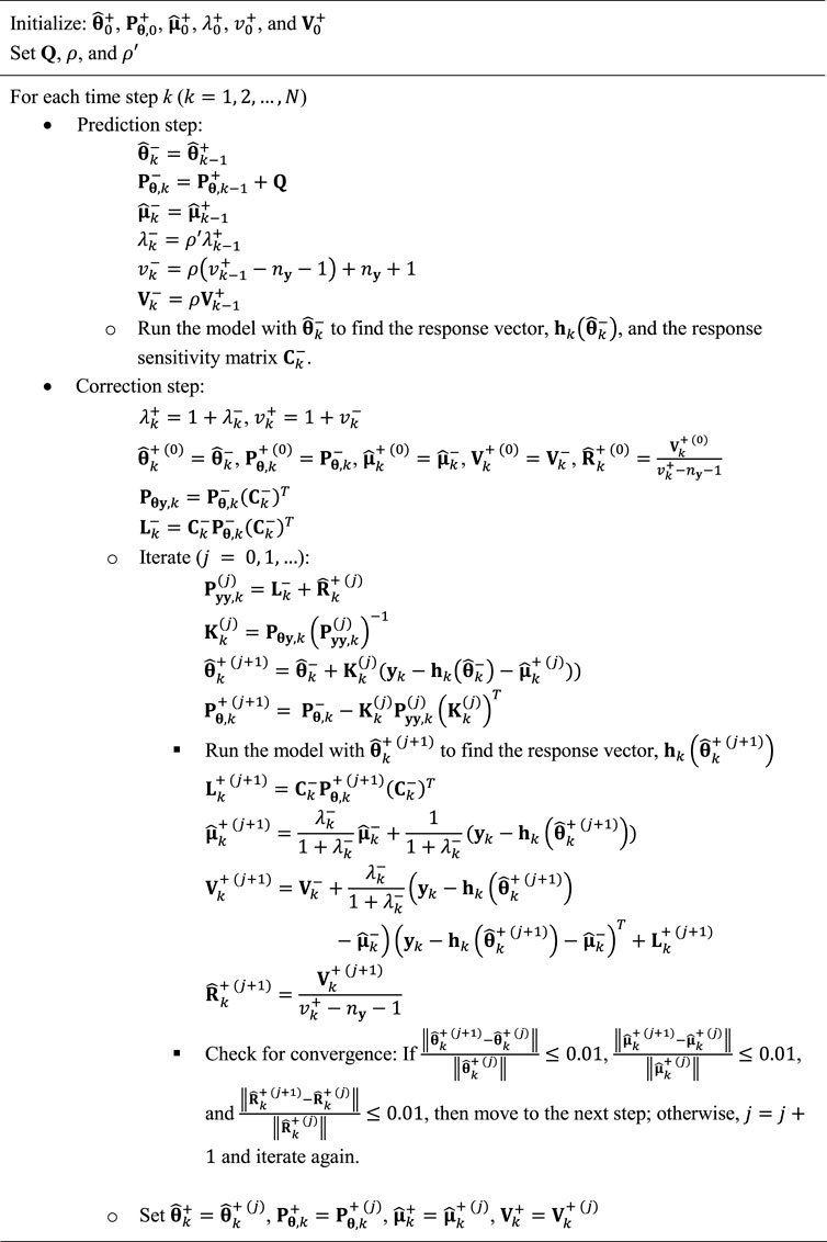
FIGURE 1. Algorithm for the recursive variational Bayesian (VB) method.

4 Comparison of the VB method with two-step marginal MAP estimation method

In this section, we compare the proposed variational Bayesian (VB) method with the two-step marginal MAP estimation method that was recently developed by Nabiyan et al. (2022) for joint estimation of unknown model parameters and the mean vector and covariance matrix of the prediction error. The formulations of the two methods are closely similar. There are two main differences between the two methods, as explained as follows. First, in the two-step marginal MAP estimation method, the mode of IW distribution is used as an ${\widehat{\mathbf{R}}}_k^{+}$ point estimate, while in the VB method, the mean of IW distribution is assigned as ${\widehat{\mathrm{R}}}_k^{+}$ (as shown in Table 1). The reason for this difference is that the MAP approach is used in the former method, while the expectation value is used in the latter. It is worth noting that the mode and mean of the IW distribution are not coincident (O'Hagan and Forster, 2004). Second, different equations are used to calculate the term ${\mathrm{V}}_k^{+}$ as shown in Table 1. The equation used to calculate ${\mathrm{V}}_k^{+}$ in the VB method has an additional term, i.e., ${\mathbf{C}}_k^{-}{\mathbf{P}}_{\mathbf{\theta },k}^{+}{\left({\mathbf{C}}_k^{-}\right)}^T$.

TABLE 1

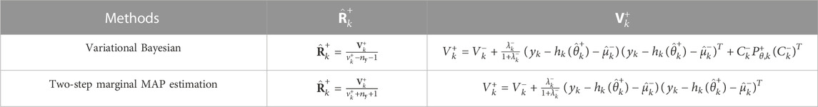
TABLE 1. Differences between the proposed VB method and two-step marginal MAP estimation method.

In most applications, these two differences have small effects on the results because of the following reasons. First, the difference between the mode and mean of the IW distribution decreases through time as the value of $v_k^{+}$ increases in time in the denominator of the characterizing equations of ${\widehat{\mathbf{R}}}_k^{+}$. Second, as the covariance matrix of the unknown model parameters ${\mathbf{P}}_{\mathbf{\theta },k}^{+}$ decreases through the Bayesian estimation (Song et al., 2020a), the effects of this additional term on the results also become negligible over time. However, the additional term ${\mathbf{C}}_k^{-}{\mathbf{P}}_{\mathbf{\theta },k}^{+}{\left({\mathbf{C}}_k^{-}\right)}^T$ in the VB method improves the estimation of ${\widehat{\mathbf{R}}}_k^{+}$ at early iterations, which in turn results in better estimation of unknown model parameters, especially when the initial estimate of the prediction error covariance matrix is poorly selected. In the next section, the estimation results of these two methods are compared through two numerical case studies.

5 Case study 1: 3-Story 1-bay steel moment frame considering time-variant measurement noise

In this section, the performance of the proposed method is evaluated when applied to a numerical model of a 3-story 1-bay steel moment frame structure under earthquake excitation. The estimation results are compared with those of the two-step marginal MAP estimation method (Nabiyan et al., 2022) and a non-adaptive Bayesian model updating method (Ebrahimian et al., 2015). The story height and the bay width are 3.5 m and 6.0 m, respectively, as shown in Figure 2A. The frame’s geometric and material properties are similar to those used in our previous work (Nabiyan et al., 2022), and more details about the considered case study can be found there.

FIGURE 2

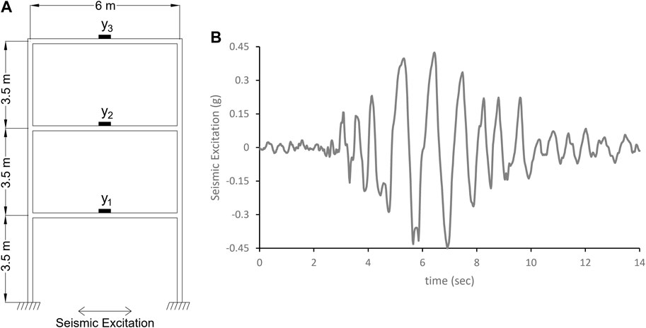
FIGURE 2. (A) 3-story 1-bay steel moment frame and (B) 0° component of ground acceleration time history of the Loma Prieta earthquake recorded at Los Gatos station (Nabiyan et al., 2022).

The numerical model of the frame is developed in OpenSees (McKenna, 2000). For this, force-based beam–column elements with seven integration points are used for columns and beams. A single fiber is used to represent each flange of beam and column cross-sections, while 10 fibers are used to discretize their webs. The uniaxial Giuffre–Menegotto–Pinto (GMP) material model (Filippou et al., 1983) with primary parameters

${\mathbf{\theta }}^{true}={\left[E_c^{true},F_{yc}^{true},b_c^{true},E_b^{true},F_{yb}^{true},b_b^{true}\right]}^T={\left[200\mathrm{G}\mathrm{P}\mathrm{a},350\mathrm{M}\mathrm{P}\mathrm{a},0.08,200\mathrm{G}\mathrm{P}\mathrm{a},250\mathrm{M}\mathrm{P}\mathrm{a},0.05\right]}^T$

is used to model the steel fibers and simulate the nominal/true dynamic response of the structure, where $E=$ Young’s modulus, $F_y=$ yield stress, and $b=$ strain-hardening ratio. The first three parameters denoted by subscript “$c$” are for columns, and the last three ones denoted by subscript “$b$” are used for beams. A nodal mass $=\mathrm{80,000}\mathrm{k}\mathrm{g}$ , shown by the black circle in Figure 2A, is considered for each story at the beam–column nodes to represent dead and live mass. To model damping energy dissipation, Rayleigh damping with 2% damping ratio is considered for the first two vibration modes of the structure.

To simulate measurement data, the frame structure is excited by the Loma Prieta earthquake (0° component at Los Gatos station), as shown in Figure 2B. Then, the horizontal absolute acceleration response time histories of each floor (shown by black boxes in Figure 2A) are extracted and contaminated with artificial measurement noise to result in simulated measurement data. The measurement noise is considered a non-stationary Gaussian random process with time-variant mean vector ${\mathbf{\mu }}_k^{true}$ and covariance matrix ${\mathbf{R}}_k^{true}$ as follows: It is worth noting that non-stationary noise with time-variant mean and covariance is a common problem in realistic monitoring, and the assumed sinusoidal form for the mean and covariance is hypothetical and considered for the feasibility study.

${\mathbf{\mu }}_k^{true}={\left[1.97,5.41,7.50\right]}^T\times \sin \left(\frac{4\pi }{N}k\right)\times {10}^{-2}g,(26)$

${\mathbf{R}}_k^{true}=\left[\begin{array}{ccc}1.66& 0& 0\\ 0& 2.88& 0\\ 0& 0& 7.65\end{array}\right]\times {\left(\sin \left(\frac{\pi }{N}k\right)+1\right)}^2\times {10}^{-4}{g}^2.(27)$

Our goal is to estimate the unknown model parameters $\mathbf{\theta }={\left[E_c,F_{yc},b_c,E_b,F_{yb},b_b\right]}^T$ and compare them with their true values ${\mathbf{\theta }}^{true}$. The initial estimate of the unknown model parameters and its covariance matrix are selected as ${\widehat{\mathbf{\theta }}}_0^{+}={\left[0.7E_c^{true},0.7F_{yc}^{true},1.2b_c^{true},0.8E_b^{true},1.3F_{yb}^{true},0.8b_b^{true}\right]}^T$ and ${\mathbf{P}}_{\mathbf{\theta },0}^{+}=\mathrm{d}\mathrm{i}\mathrm{a}\mathrm{g}{\left(0.2{\widehat{\mathbf{\theta }}}_0^{+}\right)}^2$, respectively. The initial mean vector and covariance matrix of the prediction error (measurement noise) are, respectively, assumed as ${\widehat{\mathbf{\mu }}}_0^{+}=\mathbf{0}$; ${\widehat{\mathbf{R}}}_0^{+}={10}^{-5}{\mathbf{I}}_{3\times 3}$, where ${\mathbf{I}}_{3\times 3}$ is the identity matrix. Other initial parameters of the NIW distribution are selected as ${\lambda }_0^{+}=1$, $v_0^{+}=4.1$, and ${\mathbf{V}}_0^{+}=\left(v_0^{+}-n_{\mathbf{y}}-1\right){\widehat{\mathbf{R}}}_0^{+}$, with $n_{\mathbf{y}}=3$. The process noise covariance matrix is selected as $\mathbf{Q}=\mathrm{d}\mathrm{i}\mathrm{a}\mathrm{g}{\left({10}^{-4}{\widehat{\mathbf{\theta }}}_0^{+}\right)}^2$, and the forgetting factor parameters used for defining the dynamic model of the mean vector and covariance matrix of the prediction error are assumed as $\rho =0.95$ and ${\rho }^{\prime }=0.95$, respectively Based on our study, the parameter estimation results are acceptable for $0.8\le \rho <1$ and $0.7\le {\rho }^{\prime }<1$. However, choosing lower values for $\rho$ and ${\rho }^{\prime }$ may deteriorate the performance of the model updating process. The sensitivity of the estimation process to other filter tuning parameters (e.g., initial model parameter values, $\mathbf{Q}$,) has been the subject of another study presented in Astroza et al., (2019b).

Now, the proposed VB method is applied to jointly estimate the unknown model parameter vector $\mathbf{\theta }$ and the mean vector and covariance matrix of prediction error. In this verification study, the results are compared with those of the two-step marginal MAP estimation method (Nabiyan et al., 2022) and the non-adaptive Bayesian model updating method (Ebrahimian et al., 2015) when using the same initial values. As mentioned before, in the non-adaptive Bayesian method, a zero-mean Gaussian white noise with a time-invariant diagonal covariance matrix is assumed for the prediction error ${\mathbf{\omega }}_k$, i.e., ${\mathbf{\omega }}_k\sim N\left(\mathbf{0},{\mathbf{R}}_k={\widehat{\mathbf{R}}}_0^{+}\right)$.

The estimated components of the mean vector and covariance matrix of the prediction error (measurement noise in this example) by the three methods (VB, two-step marginal MAP, and the non-adaptive) are compared with their true values in Figure 3 and Figure 4, respectively. The non-adaptive Bayesian model updating method, as mentioned before, does not estimate the mean vector and the covariance matrix of the prediction error, so they remain constant during the estimation process. However, both the VB and the two-step marginal MAP estimation methods can accurately track the trend of the true/nominal mean and covariance of error through time. As can be seen in Figure 4, in comparison to the two-step marginal MAP method, the VB method better estimates the covariance matrix of the prediction error at the early time steps because of the additional term discussed in the previous section.

FIGURE 3

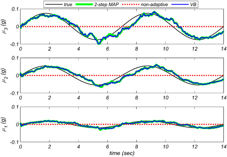
FIGURE 3. Comparison of the estimated components of the mean vector of measurement noise by the three methods (VB, two-step marginal MAP, and the non-adaptive) with the true ones. It should be noted that $\mathbf{\mu }={\left[\begin{array}{ccc}{\mathit{\mu }}_{\mathbf{1}}& {\mathit{\mu }}_{\mathbf{2}}& {\mathit{\mu }}_{\mathbf{3}}\end{array}\right]}^{\mathit{T}}.$

FIGURE 4

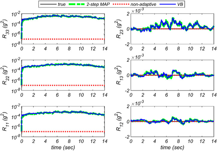
FIGURE 4. Comparison of the estimated components of the covariance matrix of measurement noise by the three methods (VB, two-step marginal MAP, and the non-adaptive) with the true ones. It should be noted that $\mathbf{R}=\left[\begin{array}{ccc}{\mathit{R}}_{\mathbf{11}}& {\mathit{R}}_{\mathbf{12}}& {\mathit{R}}_{\mathbf{13}}\\ {\mathit{R}}_{\mathbf{12}}& {\mathit{R}}_{\mathbf{22}}& {\mathit{R}}_{\mathbf{23}}\\ {\mathit{R}}_{\mathbf{13}}& {\mathit{R}}_{\mathbf{23}}& {\mathit{R}}_{\mathbf{33}}\end{array}\right]$.

Figure 5 shows the time histories of the unknown model parameters estimated by all three methods: the proposed VB method, the two-step marginal MAP estimation method, and the non-adaptive Bayesian method. It can be observed that the non-adaptive model updating method converges to incorrect unknown model parameters, or even diverges. However, adaptive methods can estimate unknown model parameters very well. The weakness of the non-adaptive method shows that estimation of the prediction error significantly affects the model updating results when the prediction error has a time-variant non-zero mean and, therefore, should not be ignored. Comparing the VB method with the two-step marginal MAP estimation method, the VB method better estimates the parameter $b_c$ (columns strain-hardening ratio) because of the better estimation of the covariance matrix of the prediction error at the early time steps.

FIGURE 5

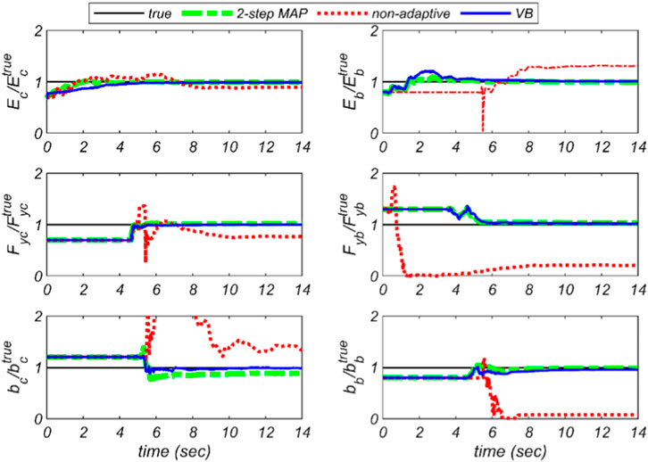
FIGURE 5. Time histories of the estimated model parameters obtained by the three methods: the proposed VB method, the two-step marginal MAP estimation method, and the non-adaptive Bayesian method.

6 Case study 2: 3-Story 3-bay steel moment frame considering modeling error

In this second study, we examine the proposed VB method in the presence of modeling error on a 3-story, 3-bay steel moment frame. The frame is taken from Song et al., (2020a), and the geometry, frame sections, and loads are shown in Figure 6. All beams and columns have wide flange profiles and are modeled with displacement-based beam–column elements. Rayleigh damping with 2% damping of the first and second modes is considered for structural damping. Distributed gravity loads are considered concentrated masses at nodes. The measured data are simulated using the steel constitutive model of Giuffre–Menegotto–Pinto (GMP) for beams and columns, in which their true properties are selected the same as in the previous example. The frame is excited by the Loma Prieta earthquake shown in Figure 2B, and the horizontal absolute acceleration responses at each floor (marked by black boxes in Figure 6) are recorded. Then, 1% RMS NSR Gaussian zero-mean white noise is added to these simulated acceleration responses to be considered measurement data.

FIGURE 6

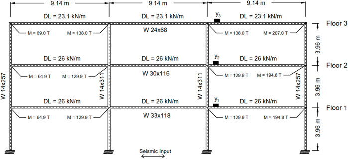
FIGURE 6. 3-Story 3-bay steel moment frame.

While we use the GMP constitutive model Figure 7A to simulate the measurements, a bilinear model (Figure 7B) is used in the estimation process to add explicit modeling error to the model updating process.

FIGURE 7

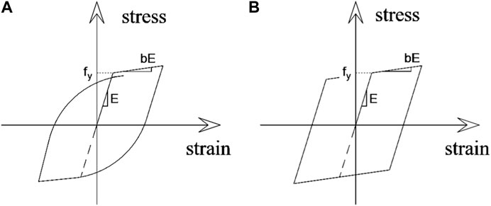
FIGURE 7. Material model (A) GMP used for simulating responses and (B) bilinear used in the estimation process.

For model updating in this example, the material properties of columns and beams are considered unknown model parameters, similar to the previous example. The initial estimate for the unknown model parameters and its covariance matrix are selected as ${\widehat{\mathbf{\theta }}}_0^{+}={\left[0.8E_c^{true},1.2F_{yc}^{true},1.4b_c^{true},0.8E_b^{true},1.2F_{yb}^{true},1.4b_b^{true}\right]}^T$ and ${\mathbf{P}}_{\mathbf{\theta },0}^{+}=\mathrm{d}\mathrm{i}\mathrm{a}\mathrm{g}{\left(0.2{\widehat{\mathbf{\theta }}}_0^{+}\right)}^2$, respectively. The initial mean vector and covariance matrix of the prediction error are assumed as ${\widehat{\mathbf{\mu }}}_0^{+}=\mathbf{0}$ and ${\widehat{\mathbf{R}}}_0^{+}={10}^{-4}{\mathbf{I}}_{3\times 3}$, respectively. As mentioned before, the non-adaptive method does not update these two parameters and considers them constants during the estimation process. Other initial parameters of the NIW distribution required for both adaptive methods are selected as ${\lambda }_0^{+}=1$, $v_0^{+}=4.1$, and ${\mathbf{V}}_0^{+}=\left(v_0^{+}-n_{\mathbf{y}}-1\right){\widehat{\mathbf{R}}}_0^{+}$, with $n_{\mathbf{y}}=3$. The process noise covariance matrix is selected as $\mathbf{Q}=\mathrm{d}\mathrm{i}\mathrm{a}\mathrm{g}{\left({10}^{-4}{\widehat{\mathbf{\theta }}}_0^{+}\right)}^2$, and the forgetting factor parameters used for defining the dynamic model of the mean vector and covariance matrix of the prediction error are assumed as $\rho =0.9$ and ${\rho }^{\prime }=0.98$.

Figure 8 shows the model updating results for the three methods: the proposed VB method, the two-step marginal MAP estimation method, and the non-adaptive Bayesian method. As can be seen, the non-adaptive method cannot estimate unknown model parameters correctly for all parameters, except $E_b$ and $E_c$. The measured structural responses are less sensitive to parameters $F_y$ and $b$, rather than $E$, which results in estimation of $F_y$ and $b$ being more effected by prediction error (measurement noise + modeling error). The non-adaptive method limits the prediction error to a zero-mean and has fixed covariance matrix. However, adaptive methods release this assumption by updating the statistical parameters of the prediction error recursively at each time step, which results in far better estimations for unknown model parameters. In comparison with the proposed adaptive VB method with the two-step marginal MAP estimation method, the VB method improved the estimation values of column and beam stiffness hardening $b_c$ and $b_b$ because of better estimation of prediction error.

FIGURE 8

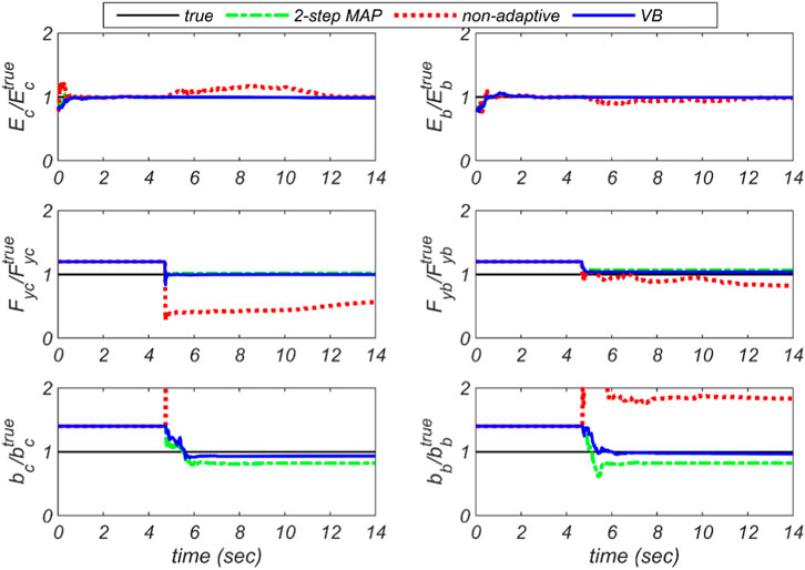
FIGURE 8. Time histories of the estimated model parameters obtained by the three methods: the proposed VB method, two-step marginal MAP estimation method, and the non-adaptive Bayesian method for the second case study.

To investigate the capability of the updated model with material modeling error in predicting the responses, absolute acceleration responses at each floor and moment–curvature response at the base of the first story’s inner column are predicted from the updated model using all three methods and compared with their true counterparts in Figure 9 and Figure 10, respectively. Although, as can be seen in Figure 9, the discrepancies between measured and predicted acceleration responses are minimized, and the estimated parameters are biased for the case of non-adaptive, and to a lesser extent for the two-step MAP method. As can be observed in Figure 10, the response predictions are considerably improved by both adaptive methods, and their predictions agree with the true moment–curvature response. Comparing the proposed VB method with the two-step MAP method, the VB method better predicts the response because of better estimation of unknown model parameters.

FIGURE 9

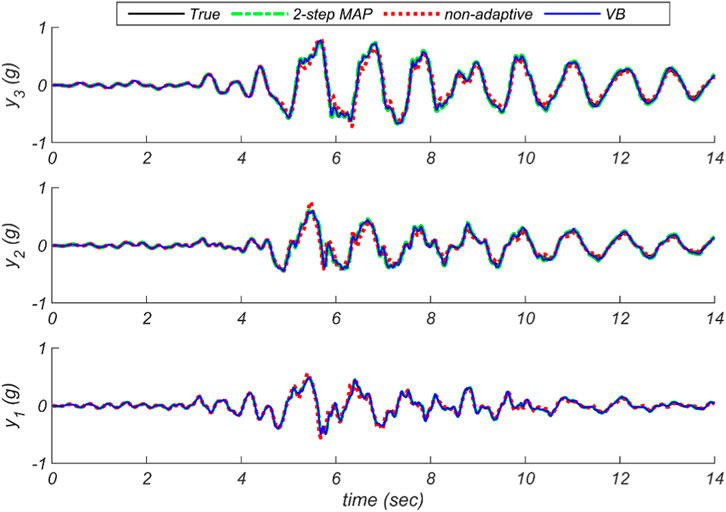
FIGURE 9. Absolute acceleration responses at each floor obtained by the true model and the updated ones using the three methods: the proposed VB method, the two-step marginal MAP estimation method, and the non-adaptive Bayesian method.

FIGURE 10

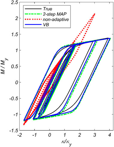
FIGURE 10. Moment–curvature responses at the base of the inner column obtained by the true model and the updated one using the three methods: the proposed VB method, the two-step marginal MAP estimation method, and the non-adaptive Bayesian method.

7 Conclusion

In this paper, we exploited the variational Bayesian (VB) approach and proposed an adaptive variational Bayesian model updating method for joint model and noise identification. A detailed mathematical derivation is provided in the paper. The performance of the proposed method is demonstrated through two numerical case studies. Two non-linear steel moment frames subjected to earthquake excitation were used, in which six parameters characterizing the constitutive models of the steel beams and columns were considered unknown. In the first case study, absolute acceleration responses at each floor contaminated by Gaussian noise with a time-variant mean vector and covariance matrix were considered measurement data. For considering modeling error in the second case study, a steel constitutive model of Giuffre–Menegotto–Pinto (GMP) is used for data simulation, and a bilinear constitutive model is used in the estimation process. The estimation results of both case studies showed that the proposed VB-based method performs well in the presence of time-variant prediction error (measurement noise and modeling error). The proposed VB-based method was also compared to a recently developed two-step marginal MAP estimation method, and the non-adaptive Bayesian model updating method. The results showed that both adaptive methods have comparable performance, while the non-adaptive method resulted in significantly biased estimations due to the adverse effects of non-stationary prediction error. The future scope of this work is to extend the algorithm to estimate the dynamic inputs, which will result in a joint input–parameter–noise estimation, and to validate the algorithm in real-world applications where the modeling errors can result in divergence or significant bias in regular model updating algorithms.

Data availability statement

The raw data supporting the conclusion of this article will be made available by the authors without undue reservation.

Author contributions

HE and M-SN conceptualized the framework. M-SN and MS derived the formulations. HE and BM verified the derivations. M-SN and MS implemented the formulation and analyzed the results. BM and HE investigated the results. M-SN and MS developed the first draft. HE and BM revised and edited. HE and BM supervised the project.

Acknowledgments

The fourth author acknowledges partial support for this study through the National Science Foundation Grant 1903972. The opinions, findings, and conclusions expressed in this paper are those of the authors and do not necessarily represent the views of the sponsors.

Conflict of interest

Author MS was employed by Gavin and Doherty Geosolutions Ltd.

The remaining authors declare that the research was conducted in the absence of any commercial or financial relationships that could be construed as a potential conflict of interest.

Publisher’s note

All claims expressed in this article are solely those of the authors and do not necessarily represent those of their affiliated organizations, or those of the publisher, the editors, and the reviewers. Any product that may be evaluated in this article, or claim that may be made by its manufacturer is not guaranteed or endorsed by the publisher.

Supplementary material

The Supplementary Material for this article can be found online at: https://www.frontiersin.org/articles/10.3389/fbuil.2023.1143597/full#supplementary-material

References

Akhlaghi, S., Zhou, N., and Huang, Z. (July 2017). Adaptive adjustment of noise covariance in Kalman filter for dynamic state estimation, Proceedings of the 2017 IEEE power and energy society general meeting (IEEE). Chicago, IL, USA. doi:10.1109/PESGM.2017.8273755

CrossRef Full Text | Google Scholar

Amini Tehrani, H., Bakhshi, A., and Yang, T. T. (2020). Online probabilistic model class selection and joint estimation of structures for post-disaster monitoring. J. Vib. Control 27, 1860–1878. doi:10.1177/1077546320949115

CrossRef Full Text | Google Scholar

Astroza, R., Alessandri, A., and Conte, J. P. (2019). A dual adaptive filtering approach for nonlinear finite element model updating accounting for modeling uncertainty. Mech. Syst. Signal Process 115, 782–800. doi:10.1016/j.ymssp.2018.06.014

CrossRef Full Text | Google Scholar

Astroza, R., Ebrahimian, H., and Conte, J. P. (2014). Material parameter identification in distributed plasticity FE models of frame-type structures using nonlinear stochastic filtering. J. Eng. Mech. 141 (5), 4014149. doi:10.1061/(ASCE)EM.1943-7889.0000851

CrossRef Full Text | Google Scholar

Astroza, R., Ebrahimian, H., and Conte, J. P. (2017). “Batch and recursive bayesian estimation methods for nonlinear structural system identification,” in Risk and reliability analysis: Theory and applications. Springer series in reliability engineering. Editor P. Gardoni (Berlin, Germany: Springer), 341–364. doi:10.1007/978-3-319-52425-2_15

CrossRef Full Text | Google Scholar

Astroza, R., Ebrahimian, H., and Conte, J. P. (2019b). Performance comparison of Kalman−based filters for nonlinear structural finite element model updating. J. Sound. Vib. 438, 520–542. doi:10.1016/j.jsv.2018.09.023

CrossRef Full Text | Google Scholar

Beal, M. J. (2003). Variational algorithms for approximate Bayesian inference: Dissertation. University of London, University, London UK.

Google Scholar

Beck, J. L., and Yuen, K.-V. (2004). Model selection using response measurements: Bayesian probabilistic approach. J. Eng. Mech. 130 (2), 192–203. doi:10.1061/(asce)0733-9399(2004)130:2(192)

CrossRef Full Text | Google Scholar

Behmanesh, I., Moaveni, B., Lombaert, G., and Papadimitriou, C. (2015). Hierarchical Bayesian model updating for structural identification. Mech. Syst. Signal Process 64, 360–376. doi:10.1016/j.ymssp.2015.03.026

CrossRef Full Text | Google Scholar

Bishop, C. M., and Nasrabadi, N. M. (2006). Pattern recognition and machine learning. New York, NY, USA: Springer.

Google Scholar

Cesmd, (2019). Center for engineering strong motion data, cesmd- A cooperative effort. https://strongmotioncenter.org.

Google Scholar

Ching, J., Beck, J. L., and Porter, K. A. (2006). Bayesian state and parameter estimation of uncertain dynamical systems. Probabilistic Eng. Mech. 21 (1), 81–96. doi:10.1016/j.probengmech.2005.08.003

CrossRef Full Text | Google Scholar

Deisenroth, M. P., Faisal, A. A., and Ong, C. S. (2020). Mathematics for machine learning. Cambridge University Press, Cambridge, UK.

Google Scholar

Doebling, S. W., Farrar, C. R., Prime, M. B., and Shevitz, D. W. (1996). Damage identification and health monitoring of structural and mechanical systems from changes in their vibration characteristics: A literature review. NM, USA: Los Alamos National Lab. doi:10.2172/249299

CrossRef Full Text | Google Scholar

Ebrahimian, H., Astroza, R., and Conte, J. P. (2015). Extended Kalman filter for material parameter estimation in nonlinear structural finite element models using direct differentiation method. Earthq. Eng. Struct. Dyn. 44 (10), 1495–1522. doi:10.1002/eqe.2532

CrossRef Full Text | Google Scholar

Filippou, F. C., Popov, E. P., and Bertero, V. V. (1983). Effects of bond deterioration on hysteretic behavior of reinforced concrete joints. EERC 83–19. Earthquake Engineering Research Center. Berkeley, CA, USA: Univ. of California.

Google Scholar

Friswell, M., and Mottershead, J. E. (2013). Finite element model updating in structural dynamics. Springer Science and Business Media, Berlin, Germany.

Google Scholar

Granström, K., and Orguner, U. (2011). Properties and approximations of some matrix variate probability density functions. Linköping University Electronic Press, Linköping, Sweden.

Google Scholar

Haykin, S. (2004). Kalman filtering and neural networks. John Wiley and Sons, New York, NY, USA.

Google Scholar

Huang, Y., Yu, J., Beck, J. L., Zhu, H., and Li, H. (2020). Novel sparseness-inducing dual Kalman filter and its application to tracking time-varying spatially-sparse structural stiffness changes and inputs. Comput. Methods Appl. Mech. Eng. 372, 113411. doi:10.1016/j.cma.2020.113411

CrossRef Full Text | Google Scholar

Huang, Y., Zhang, Y., Li, N., and Zhao, L. (2016). Design of sigma-point Kalman filter with recursive updated measurement. Int. J. Circuits, Syst. Signal Process. 35 (5), 1767–1782. doi:10.1007/s00034-015-0137-y

CrossRef Full Text | Google Scholar

Huang, Y., Zhang, Y., Wu, Z., Li, N., and Chambers, J. (2017). A novel adaptive Kalman filter with inaccurate process and measurement noise covariance matrices. IEEE T Autom. Contr 63 (2), 594–601. doi:10.1109/TAC.2017.2730480

CrossRef Full Text | Google Scholar

Kollo, T., and Von Rosen, D. (2006). Advanced multivariate statistics with matrices. Springer Science and Business Media, Berlin, Germany.

Google Scholar

Kontoroupi, T., and Smyth, A. W. (2016). Online noise identification for joint state and parameter estimation of nonlinear systems. ASCE-ASME J. Risk Uncertain. Eng. Syst. A Civ. Eng. 2 (3), B4015006. doi:10.1061/AJRUA6.0000839

CrossRef Full Text | Google Scholar

Law, K. J., and Stuart, A. M. (2012). Evaluating data assimilation algorithms. Mon. Weather Rev. 140 (11), 3757–3782. doi:10.1175/mwr-d-11-00257.1

CrossRef Full Text | Google Scholar

McKenna, F., Fenves, G. L., and Scott, M. H. (2000). Open system for earthquake engineering simulation. Berkeley, CA, USA: University of California.

Google Scholar

Mehra, R. (1972). Approaches to adaptive filtering. IEEE T Autom. Contr 17 (5), 693–698. doi:10.1109/tac.1972.1100100

CrossRef Full Text | Google Scholar

Nabiyan, M. S., Ebrahimian, H., Moaveni, B., and Papadimitriou, C. (2022). Adaptive bayesian inference framework for joint model and noise identification. J. Eng. Mech. 148 (3), 4021165. doi:10.1061/(ASCE)EM.1943-7889.0002084

CrossRef Full Text | Google Scholar

Nabiyan, M. S., Khoshnoudian, F., Moaveni, B., and Ebrahimian, H. (2020). Mechanics-based model updating for identification and virtual sensing of an offshore wind turbine using sparse measurements. Struct. Contr. Health Monit. 28, e2647. doi:10.1002/stc.2647

CrossRef Full Text | Google Scholar

O'Hagan, A., and Forster, J. J. (2004). Kendall's advanced theory of statistics, 2. 2, Arnold, London, UK.

Google Scholar

Opper, M., and Saad, D. (2001). Advanced mean field methods: Theory and practice. MIT Press, Cambridge, MA, USA.

Google Scholar

Paolella, M. S. (2018). Linear models and time-series analysis: Regression, ANOVA, ARMA and GARCH. John Wiley and Sons, New York, NY, USA.

Google Scholar

Song, M., Behmanesh, I., Moaveni, B., and Papadimitriou, C. (2020). Accounting for modeling errors and inherent structural variability through a hierarchical bayesian model updating approach: An overview. Sensors 20 (14), 3874. doi:10.3390/s20143874

PubMed Abstract | CrossRef Full Text | Google Scholar

Sanayei, M., Arya, B., Santini, E. M., and Wadia-Fascetti, S. (2001). Significance of modeling error in structural parameter estimation. COMPUT-AIDED Civ. Inf. 16 (1), 12–27. doi:10.1111/0885-9507.00210

CrossRef Full Text | Google Scholar

Sarkka, S., and Hartikainen, J. (September 2013). Non-linear noise adaptive Kalman filtering via variational Bayes, Proceedings of the 2013 IEEE international workshop on machine learning for signal processing (MLSP), (IEEE), Southampton, UK.

Google Scholar

Sarkka, S., and Nummenmaa, A. (2009). Recursive noise adaptive Kalman filtering by variational Bayesian approximations. IEEE T Autom. Contr 54 (3), 596–600. doi:10.1109/TAC.2008.2008348

CrossRef Full Text | Google Scholar

Shi, Y., Tang, X., Feng, X., Bian, D., and Zhou, X. (2018). Hybrid adaptive cubature Kalman filter with unknown variance of measurement noise. Sensors 18 (12), 4335. doi:10.3390/s18124335

PubMed Abstract | CrossRef Full Text | Google Scholar

Šmídl, V., and Quinn, A. (2006). The variational Bayes method in signal processing. Springer Science and Business Media, Berlin, Germany.

Google Scholar

Song, M., Astroza, R., Ebrahimian, H., Moaveni, B., and Papadimitriou, C. (2020). Adaptive Kalman filters for nonlinear finite element model updating. Mech. Syst. Signal Process 143, 106837. doi:10.1016/j.ymssp.2020.106837

CrossRef Full Text | Google Scholar

Sun, C., Zhang, Y., Wang, G., and Gao, W. (2018). A new variational Bayesian adaptive extended Kalman filter for cooperative navigation. Sensors 18 (8), 2538. doi:10.3390/s18082538

PubMed Abstract | CrossRef Full Text | Google Scholar

Sun, J., Zhou, J., and Gu, X. (2012). Variational Bayesian two-stage Kalman filter for systems with unknown inputs. Procedia Eng. 29, 2265–2273. doi:10.1016/j.proeng.2012.01.299

CrossRef Full Text | Google Scholar

Tzikas, D. G., Likas, A. C., and Galatsanos, N. P. (2008). The variational approximation for Bayesian inference. IEEE Signal Process. Mag. 25 (6), 131–146. doi:10.1109/MSP.2008.929620

CrossRef Full Text | Google Scholar

Weinstock, R. (1974). Calculus of variations: With applications to physics and engineering. Dover Publications, New York.

Google Scholar

Wenzel, T., Burnham, K., Blundell, M., and Williams, R. (2007). Kalman filter as a virtual sensor: Applied to automotive stability systems. Trans. Inst. Meas. Control 29 (2), 95–115. doi:10.1177/0142331207072990

CrossRef Full Text | Google Scholar

Wu, J. (2005). Some properties of the normal distribution. https://cs.nju.edu.cn/_upload/tpl/00/ed/237/template237/paper/Gaussian.pdf.

Google Scholar

Wu, M., and Smyth, A. W. (2007). Application of the unscented Kalman filter for real-time nonlinear structural system identification. Struct. Contr. Health Monit. 14 (7), 971–990. doi:10.1002/stc.186

CrossRef Full Text | Google Scholar

Xu, D., Wu, Z., and Huang, Y. (2019). A new adaptive Kalman filter with inaccurate noise statistics. Int. J. Circuits, Syst. Signal Process. 38 (9), 4380–4404. doi:10.1007/s00034-019-01053-w

CrossRef Full Text | Google Scholar

Yang, J. N., Lin, S., Huang, H., and Zhou, L. (2006). An adaptive extended Kalman filter for structural damage identification. Struct. Contr. Health Monit. 13 (4), 849–867. doi:10.1002/stc.84

CrossRef Full Text | Google Scholar

Yuen, K. V., and Kuok, S. C. (2016). Online updating and uncertainty quantification using nonstationary output-only measurement. Mech. Syst. Signal Process 66, 62–77. doi:10.1016/j.ymssp.2015.05.019

CrossRef Full Text | Google Scholar

Zhang, Q., Yang, Y., Xiang, Q., He, Q., Zhou, Z., and Yao, Y. (2018). Noise adaptive Kalman filter for joint polarization tracking and channel equalization using cascaded covariance matching. IEEE Photonics J. 10 (1), 1–11. doi:10.1109/JPHOT.2018.2797050

CrossRef Full Text | Google Scholar

Zheng, B., Fu, P., Li, B., and Yuan, X. (2018). A robust adaptive unscented Kalman filter for nonlinear estimation with uncertain noise covariance. Sensors 18 (3), 808. doi:10.3390/s18030808

PubMed Abstract | CrossRef Full Text | Google Scholar