Assessing the transport connectivity of urban territories, based on intermodal transport accessibility

1 Introduction

Transport connectivity of urban areas is an interdisciplinary concept. In many cases, this indicator is very important for assessing the quality of life in cities. Due to the growing popularity of the concept of “connectivity” in transport, economic, and geographical scientific works, there is an important question: “What is connected to what?” (ESCAP, 2019). The United Kingdom National Infrastructure Commission defines connectivity as “the ease with which people can get around within (Intra-urban connectivity), and between (Inter-urban connectivity) different places.” (NIC, 2021). However, depending on the objectives of measuring connectivity, there are other definitions of connectivity.

In the transportation literature, connectivity is viewed as a measure in which passenger and freight flows can reach other nodes from one node either directly or indirectly through other nodes (Rodrigue, 2020). In the context of urban transport, the concept of connectivity of the street and road network prevails, which is defined as the number of roads and tracks connecting one area to another (ESCAP, 2019).

There are many concepts and measures of connectivity, that are typically expressed in relation to the transport network topology. The main objective of any transportation network is to establish connectivity, which facilitates the linkage of places that individuals intend to travel to and from. The study of transport connectivity is directly related to the representation of transport networks in graph form (Rodrigue, 2020). There are measures that evaluate the connectivity of transport networks as dimensionless ratios: Alpha, Beta/Inter-connectivity index (Kansky, 1963; Ewing, 1996; Saikia and Kar, 2023), Gamma, network diameter, and others (Kansky, 1963; Saikia and Kar, 2023). New metrics were added to these measures, taking into account the travel time (Lam and Schuler, 1981). Detour index shows the distance/time ratio by a straight line and by road network between two sections (Guze, 2019). Some models combine indicators of demand for correspondence and different types of transfers (Hadas and Ceder, 2010; Kurlov et al., 2022).

Furthermore, there is also a social component of connectivity. Transport networks along with connectivity play an important role in enabling the poor to access fundamental needs like employment, education, and healthcare (Mattioli et al., 2017). By this transport networks can help to reduce poverty (Jiang et al., 2020). However, Hernandez and Dávila (2016) found that while connectivity can indeed be an important factor in overcoming poverty in physically marginal areas these areas are often bypassed in the process of designing connectivity networks due to lack of power and influence of its inhabitants on political decisions.

In transport studies, connectivity assessment methods combine not only the characteristics of the road network. Some models combine indicators of demand for correspondence and different types of transfers (Hadas and Ceder, 2010; Kurlov et al., 2022). Other models require more complex datasets such as demographics, demand, transportation zones, centers of attractions, and more. More comprehensive studies can be found in the field of connectivity of the public transport network, where the social needs of people, the difference in the accessibility of public transport depending on the territory, can be taken into account (Currie, 2010; Bolleter et al., 2021).

The road or public transit network can also form a barrier for connectivity. The road network obviously connects urban areas with each other, but the complex structure of the city and the entire road network leads to some areas may have poorer connections to surrounding land uses. Areas with many cul-de-sacs in the road network may be poorly connected to downtown or other outlying parts of the city, as it will take longer to reach them than crow-fly from block to block (Litman, 2009; Rodrigue, 2020). The number of connections of the area to the entire street and road network also determines the time of travel or commuting (Levinson, 2012). Commute time is the normal time spent by people traveling from home to their work (Sridhar and Nayka, 2022). There is still no single unified standard for how much time a person on average should spend moving around the city or going to work. This was first mentioned by Marchetti, where he identified a constant of 1 h to get from home to work and back (Marchetti, 1994). The city may grow and sprawl, but the travel time from the edge of the city to the center remains 30 min due to advances in technology and modes of transportation (Marchetti, 1994). However, in today’s environment, some studies based on GPS data on the movements of people (Rhee et al., 2011; Jia et al., 2012; Vazquez-Prokopec et al., 2013; Jin et al., 2022), data from cellular operators (Kung et al., 2014) show that in different cities of different sizes with a variety of street and road structures, the travel time around the city varies a lot, and it becomes difficult to determine the ideal “Marchetti’s constant”.

In this paper, we consider transport connectivity as the mutual transport accessibility of urban areas. Unlike other works, which evaluate intra-city transport connectivity through topological characteristics of the street and road network in graph form (Galpern et al., 2018; Scoppa et al., 2019; Scoppa and Anabtawi, 2021), we compare the values of travel time between all city blocks in a straight line (Euclidean distance) and by public transport. In contrast to the Detour index (Guze, 2019) or PRD (Scoppa et al., 2019), we consider the connectivity not of two sections of the street and road network, but of all city blocks, which in this paper act as a spatial unit of the city. This approach allows us to see which parts of the city are “cut off” from the rest through the public transportation network.

2 Materials and methods

In this work, transport connectivity of the city is assessed through travel times by Euclidean distances and public transport routes between blocks. The method is divided into three steps (Figure 1).

1. Data preparation—preprocess the necessary data to get the geometry of city blocks and the transport graph;

2. Calculating the shortest travel time between city blocks using Euclidean distances and public transportation via intermodal graph;

3. Clustering based on the resulting time values to get groups of blocks and compare them to administrative “belonging”.

FIGURE 1

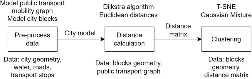
FIGURE 1. The method for assessing the transport connectivity of urban areas.

Time matrices are obtained between all the blocks. Reduce the dimensionality of the obtained data using the algorithm t-SNE (t-Distributed Stochastic Neighbor Embedding) (Maaten and Hinton, 2008). To cluster the blocks we use the Gaussian Mixture model (Reynolds et al., 2009). In this paper, the method was applied to four cities: Saint Petersburg (Russia), Helsinki (Finland), Stockholm (Sweden), and Amsterdam (Netherlands).

2.1 Pre-processing the necessary data

The first stage (Figure 2) is to upload data sets of city boundaries and administrative districts, water bodies, street and road networks to cut the city into blocks. It is necessary to cut the geometries of water bodies and roads from the geometry of the city in the administrative boundaries and add the geometries of administrative districts. It is important to clarify that not all data was obtained from OSM (OSM, 2022) in the right quality, so some data, for example, on water and/or on administrative areas of Helsinki (2022), City of Amsterdam (2022) and Stockholm (2021) were taken from national spatial data portals.

FIGURE 2

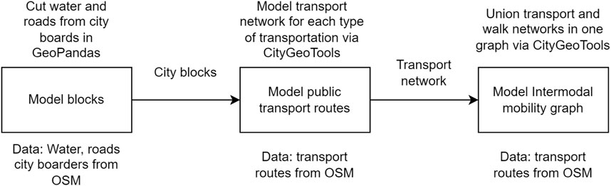
FIGURE 2. Data prepossessing algorithm.

Public transport routes and stops were also obtained with OpenStreetMap (OSM, 2022) within the administrative boundaries of the city. The intermodal graph is obtained by combining the walk graph and the graph of public transport in the vertices corresponding to stops (Mishina et al., 2022). The links in the graph are the pedestrian sections and public transport routes. The routes of different types of public transport, as well as the pedestrian graph, were connected in a single network, where the nodes are the connection points of the pedestrian sections and public transport stops. Each link of the graph is associated with a type of vehicle passing through the corresponding segment, and each node is associated with a list of modes of transport stopping at the corresponding point. The weight of the links is the time it takes to pass them.

2.2 Travel time calculation

For each city block a centroid is constructed and the nearest point of the graph is searched from it. In rare cases, the same node coincides for two blocks. Between each block (the nearest points of the graph) we look for the shortest distance from one node to another using Dijkstra’s algorithm (Kwan et al., 2003). We obtained a similarity matrix of distances between all blocks. Knowing the distances between all blocks, we calculated the minimum time to travel by public transportation (using the intermodal graph (Mishina et al., 2022)). As a result, we obtained matrices with the shortest distances and times between all the blocks that can be mapped (Figure 3). To get the Euclidean distances between blocks, we look at the distance between all blocks in a straight line from centroid to centroid.

FIGURE 3

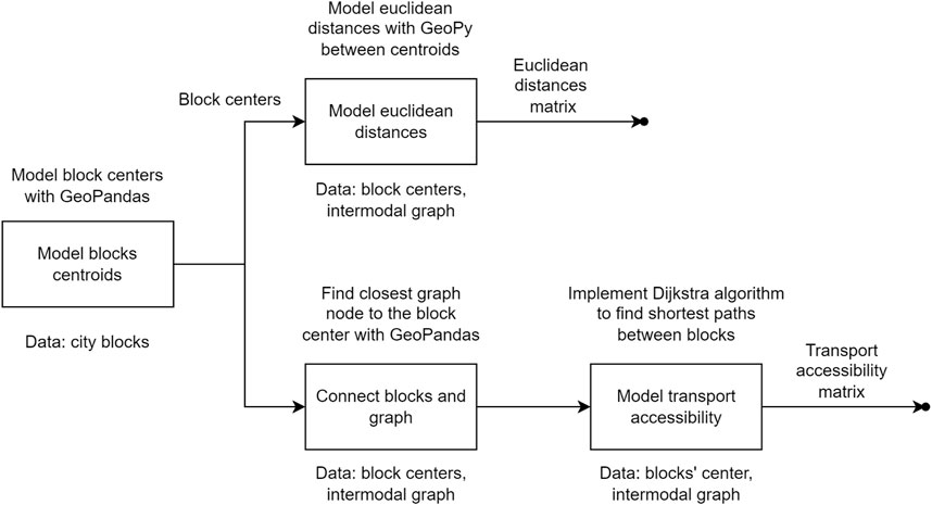
FIGURE 3. Travel time calculation algorithm.

The connection of the same blocks can be different, depending on the network on which it travels. The entire street and road network may be used for vehicular travel, except pedestrian paths. However, the urban structure and layout can be complex: for example, different parts of the city may be separated by natural barriers (rivers, forest parks, ravines, and others.), which reduces the possibility of creating an uninterrupted street and road network (Litman, 2009). One part of the city may be connected to another with only one bridge on the street and road network for movement by car, while by public transport they may be connected not only by road but also by railroad tracks or the subway network.

2.3 Clustering

To cluster blocks (Figure 4), it was necessary to reduce the dimensionality of the data and choose a clustering algorithm. To switch from matrix representation to two-dimensional representation, the dimensionality reduction algorithm t-SNE (t-Distributed Stochastic Neighbor Embedding) (Maaten and Hinton, 2008) was used with the following parameters: n_components = 2, perplexity = 100, n_iter = 1000, random state = 7575. The Gaussian Mixture Model (GMM) (Reynolds et al., 2009) is a parametric probability density function represented as a weighted sum of Gaussian component densities) with the following parameters: random_state = 7575, covariance_type = ‘diag’, init_params = ‘kmeans’ was chosen for clustering. The distribution of the data after dimensionality reduction, as well as the necessity not to exclude any point (because each characterizes a block), made it necessary to choose this method of classification. The number of clusters was selected using the Silhouette Score (Rousseeuw, 1987), which provides the selection of the best number of clusters relative to how well each object is clustered with a different number of clusters. For each cluster, the median time was calculated based on the blocks that fell into it. To compare the clusters with each other, they were sorted by increasing median time, where the first cluster was assigned green (the best connectivity) and the last cluster was assigned red (the worst connectivity). Thus, the following values were obtained for the following cities: Saint Petersburg (Russia), Helsinki (Finland), Stockholm (Sweden), and Amsterdam (Netherlands).

FIGURE 4

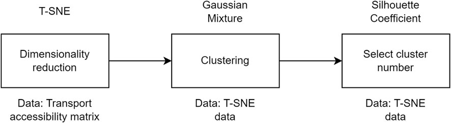
FIGURE 4. Clustering algorithm.

2.4 Experiment

The intermodal graph used in this work, for calculating travel times between blocks, is a flexible and customizable tool for estimating the transportation situation. However, we can also use this tool to model potential changes in the public transportation network. For this purpose, we have added to the intermodal graph 4 subway stations of the Green line, which are still being designed (Figure 5). The coordinates of the stops were added manually during the collection of the transport graph when combining the subway routes with the OSM into a single graph.

FIGURE 5

FIGURE 5. Added subway stations.

Next, the calculations were repeated using the proposed method. A histogram of the distribution of block accessibility was plotted. The results show an improvement in the overall connectivity of urban blocks (Figure 6).

FIGURE 6

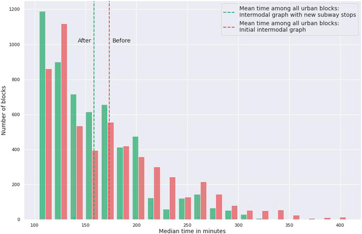
FIGURE 6. Distribution of median travel time between blocks.

3 Results

Figures 7, 8 show the results of clustering St. Petersburg blocks by travel time in a straight line between all blocks. A total of 13 clusters were obtained. The shapes of the clusters are determined by the geographical features of the city districts. Cluster 0 mainly includes such districts as Central, Admiralteisky, and part of Petrogradsky. Peripheral districts (part of Krasnoselsky, Moskovsky, Frunzensky, Vasileostrovsky) belong to clusters 1–3. Clusters of distant from the center districts are scattered on the graph and elongated because of their geographical shape. The Kurortny district is divided into 3 clusters (5, 8, 12). Cluster 12 includes the most distant part of the Kurortny district from the city center.

FIGURE 7

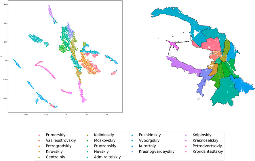
FIGURE 7. Belonging of clustered blocks to districts of Saint Petersburg (Euclidean distances).

FIGURE 8

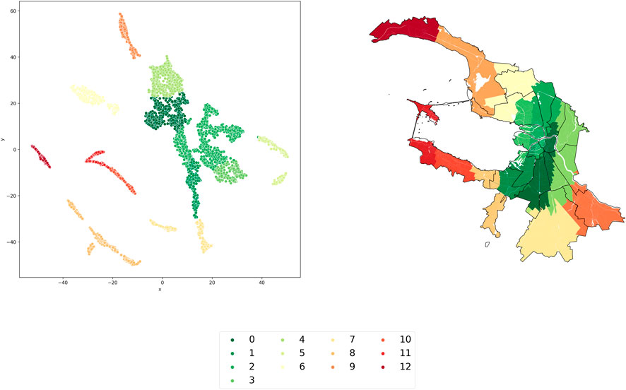
FIGURE 8. Clustering of Saint Petersburg blocks by time by Euclidean distances.

Figures 9, 10 show the results of clustering St. Petersburg blocks by the value of travel time by public transport from all to all blocks. A total of 13 clusters were obtained according to the given parameters. Clusters 0 and 1, unlike clustering by Euclidean distances, included more central districts (Central, Admiralteisky, Petrogradsky, Vasileostrovsky). With clustering, we consider the transport connectivity of the city as a mutual transport accessibility of urban areas, as mentioned above in the Introduction section. Comparing with the results of the clustering of blocks by Euclidean distances, it is possible to see how different blocks are connected to other blocks through the distance in a straight line and through the routes of public transport. For example, blocks in the Pushkin district are better connected by a straight line than by public transportation routes. This may be due to the fact that public transport infrastructure is underdeveloped in this area of the city.

FIGURE 9

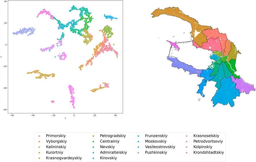
FIGURE 9. Belonging of clustered blocks to districts of Saint Petersburg (Public transport).

FIGURE 10

FIGURE 10. Clustering Saint Petersburg blocks by the time between all by public transport.

The results of the Euclidean distance clustering show that many areas in the center and on the periphery form an enclave of clusters 0–8 (Figures 7, 8). Such areas share many geographic boundaries and are close to each other. Figures 9, 10 show that these areas no longer form one enclave. Despite their geographical closeness, through public transportation, they are less accessible in time relative to each other. Vyborgsky, part of Kalininsky, and Krasnogvardeisky districts form an enclave. Central, Admiralteysky districts are connected with Moskovsky and Nevsky districts. The remote districts form several enclaves at once: part of the Krasnoselsky and part of the Petrodvortsovy districts form cluster 9 (Figure 10), and their other parts already belong to clusters 8 and 16.

Figures 11–14 show the results of the connectivity assessment for the city of Helsinki (Finland). The result of clustering blocks by travel time by Euclidean distances (Figures 11, 12) - 2 clusters. Cluster 0 combines 4 city districts such as Eteläinensuurpiiri, Läntinensuurpiiri, Keskinensuurpiiri and Pohjoinensuurpiiri.

FIGURE 11

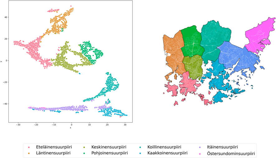
FIGURE 11. Belonging of clustered blocks to districts of Helsinki (Euclidean distances).

FIGURE 12

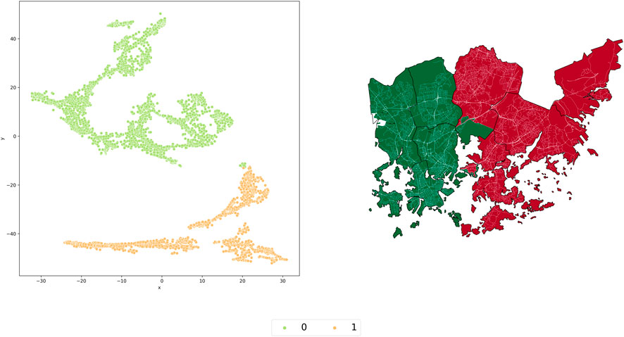
FIGURE 12. Clustering of Helsinki blocks by time by Euclidean distances.

FIGURE 13

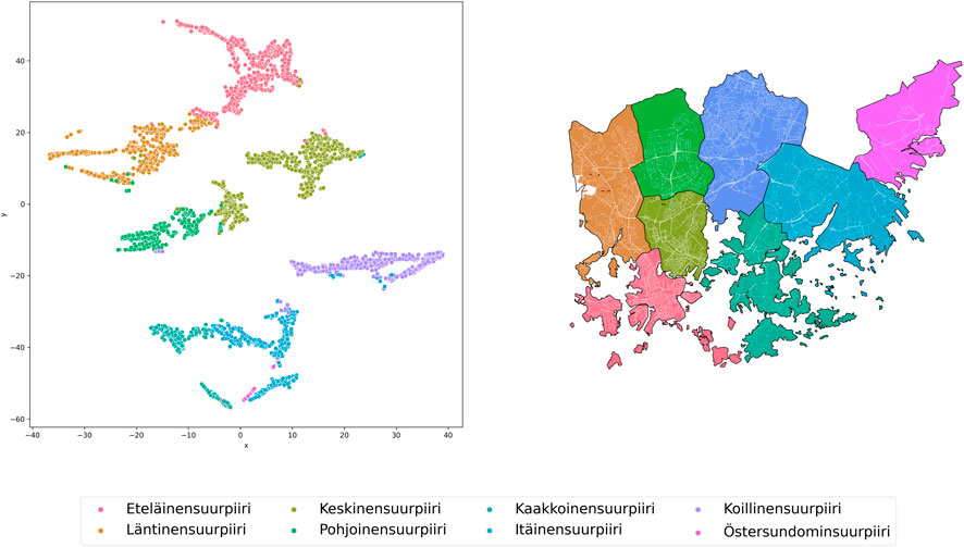
FIGURE 13. Belonging of clustered blocks to districts of Helsinki (Public transport).

FIGURE 14

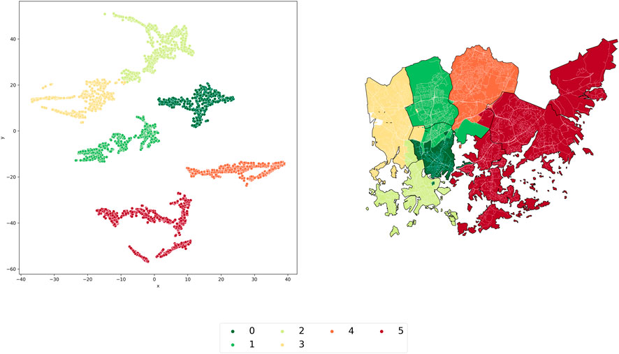
FIGURE 14. Clustering Helsinki blocks by time between all by public transport.

In terms of travel time by public transport, the blocks form 6 clusters (Figures 13, 14). Cluster 5 includes the districts most distant from the downtown of Helsinki (Östersundominsuurpiiri, Itäinensuurpiiri and Pohjoinensuurpiiri). The districts Etalainensuurpiiri, Lantinensuurpiiri, Keskinensuurpiiri and Pohjoinensuurpiiri are combined into 1 cluster enclave (0–3).

The results of clustering the travel time values by Euclidean distances and by public transport between all the blocks show that there are many natural barriers in Helsinki, which were mentioned in the Introduction section. The city is divided into 2 clusters by straight lines, as opposed to 6 by the public transportation network.

Figures 15 and Supplementary Figure S1-S3 show the results of the connectivity assessment of urban blocks in Stockholm, Sweden. Stockholm, like the cities for which the connectivity assessment was done above, has a number of natural barriers in the form of the Norrström and Söderström rivers. The connectivity of blocks by Euclidean distances and by public transport is very uneven. The urban areas of Sodermalmas, Kungsholmens and Spanga-Tensta form an enclave of 6 and 7 clusters (Supplementary Figure S3). However, some parts of these areas belong to completely different clusters. This may be due to the presence of many cul-de-sacs in the street and road network on which public transport travels. A small number of the blocks in the Hässelby-Vällingby and Bromma neighborhoods belong to clusters 0 and 1 (Supplementary Figure S3). These districts have the final subway line stations connected to the city center (clusters 0–2). Part of this subway line does not fall within the administrative boundaries of the city, so the nearby neighborhoods belong to other clusters (this paper considers connectivity only for blocks that fall within the city boundaries).

FIGURE 15

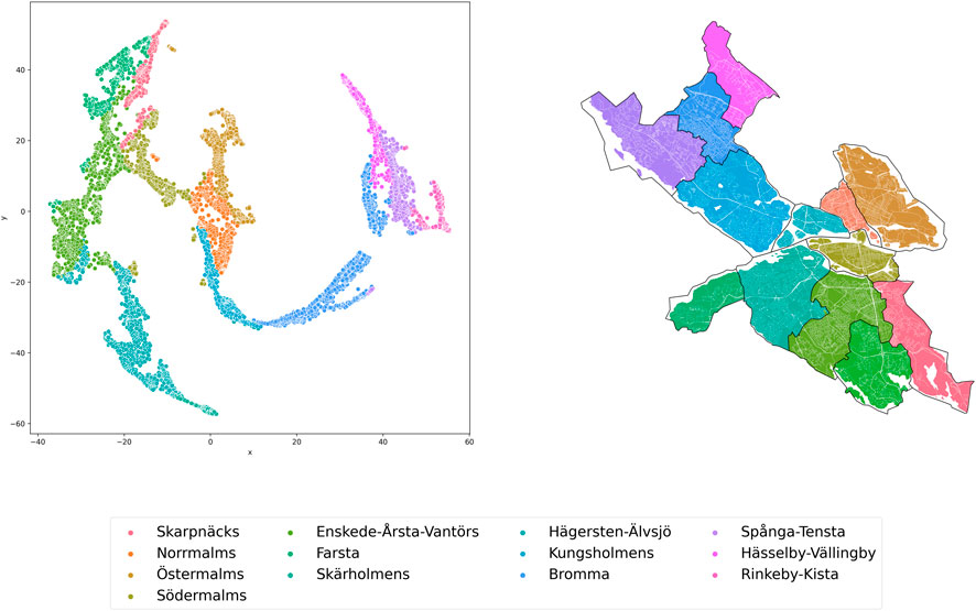
FIGURE 15. Belonging of clustered blocks to districts of Stockholm (Euclidean distances).

Supplementary Figure S4-S7 show the results of the connectivity estimation for Amsterdam (Netherlands). By Euclidean distances, the city districts are divided into 11 clusters (Supplementary Figure S5). Some districts away from the city center form enclaves of clusters, such as clusters 7 and 9. However, when evaluating connectivity by public transportation, these districts score better. The Oud-Oost neighborhood is better connected to all other parts of the city by public transportation than by direct lines (Supplementary Figure S7).

4 Discussion

The paper presents a method for assessing the connectivity of urban areas on public transport. To model the connectivity of urban areas we use open data, such as geometries of cities and routes with public transport stops, from which the intermodal graph is constructed. Transport connectivity in this paper is meant the mutual transport accessibility of urban areas. To assess the connectivity calculated median travel time from each quarter to all others in a straight line (Euclidean distance) and the network of public transport. This approach allows us to compare how urban areas can be connected to each other through travel time, in case they are physically close or distant. Applying the method to different cities revealed that, for example, in cities where there are natural barriers in the form of rivers, canals, etc., accessibility by public transport differs significantly from accessibility by a straight line, as seen in Saint Petersburg or Stockholm. On the other side, the results show that in such cities as Amsterdam and Helsinki, with a well-developed transport system, natural barriers are not always an obstacle to good transport connectivity of urban areas. This method does not take into account the entire set of data on intra-city transport. A weakness of this approach for evaluating connectivity through accessibility is the resource-intensive configuration of the intermodal graph. Since the graph is built for the whole city, it is necessary to take into account that the speeds of transport may vary in different sections due to the speed regime. The presented method makes it possible to assess the connectivity of urban areas through the public transport network. A spatial unevenness model can be constructed for specific areas. With the method, it is possible to single out the enclaves of territories, which possess greater connectivity due not only to the street and road network but also to the geography of the city (elongated districts, many rivers and channels, river sides connected with bridges, isolated islands and so on). The method can be used to make urban planning decisions about the provision of urban infrastructure, allows for ongoing monitoring of the situation and filling in the gaps.

5 Conclusion

The article presents a method for assessing the urban environment as the transport connectivity of territories. As a territorial unit of the urban environment, the city block was chosen, which most often acts as a unit of the spatial planning structure of the city. This allowed us to give greater versatility to the method, which allows us to obtain comparable estimates for different cities of the world. The obtained estimates were compared with the estimate of the remoteness of the blocks by Euclidean distance. Thus, the Euclidean distance acts as a baseline estimate. The basic assumption of the method was that the city’s transport system should give a better estimate of the city’s transport connectivity than baseline.

This assumption proved to be justified for cities where transport systems do not have natural barriers, for example, in the continental part of Helsinki. At the same time, if there are significant obstacles in the city in the form of a network of canals and rivers, the assessment turns out to be worse, as can be seen in Saint Petersburg or Amsterdam.

Thus, the proposed method can serve as a convenient and simple assessment of the quality of the organization of the city’s transport system and serve as a tool for its improvement.

Data availability statement

Publicly available datasets were analyzed in this study. This data can be found here: https://www.openstreetmap.org; https://maps.amsterdam.nl; https://dataportalen.stockholm.se; https://www.hsy.fi.

Author contributions

Literary review - AM, IS and LS. Method - GK and NZ. Description of method - AM and GK. Approbation of method - GK. Results and discussion - AM. Supervision - SB and SM. Conceptual idea - SM.

Funding

This research is financially supported by the Russian Science Foundation, Agreement 17-71-30029 (https://rscf.ru/en/project/17-71-30029/), with co-financing of Bank Saint Petersburg.

Conflict of interest

The authors declare that the research was conducted in the absence of any commercial or financial relationships that could be construed as a potential conflict of interest.

Publisher’s note

All claims expressed in this article are solely those of the authors and do not necessarily represent those of their affiliated organizations, or those of the publisher, the editors and the reviewers. Any product that may be evaluated in this article, or claim that may be made by its manufacturer, is not guaranteed or endorsed by the publisher.

Supplementary material

The Supplementary Material for this article can be found online at: https://www.frontiersin.org/articles/10.3389/fbuil.2023.1148708/full#supplementary-material

References

Bolleter, J., Vokes, R., Duckworth, A., Oliver, G., McBurney, T., and Hooper, P. (2021). Using suitability analysis, informed by Co-Design, to assess contextually appropriate urban growth models in Gulu, Uganda. uganda 27, 245–269. doi:10.1080/13574809.2021.1968295

CrossRef Full Text | Google Scholar

City of Amsterdam (2022). Maps data.

Google Scholar

Currie, G. (2010). Quantifying spatial gaps in public transport supply based on social needs. J. Transp. Geogr. 18, 31–41. doi:10.1016/j.jtrangeo.2008.12.002

CrossRef Full Text | Google Scholar

Escap, U. (2019). Enhancing rural transport connectivity to regional and international transport networks in asia and the pacific.

Google Scholar

Ewing, R. H. (1996). Pedestrian-and transit-friendly design.

Google Scholar

Galpern, P., Ladle, A., Uribe, F. A., Sandalack, B., and Doyle-Baker, P. (2018). Assessing urban connectivity using volunteered mobile phone gps locations. Appl. Geogr. 93, 37–46. doi:10.1016/J.APGEOG.2018.02.009

CrossRef Full Text | Google Scholar

Guze, S. (2019). Graph Theory Approach to the Vulnerability of Transportation Networks. Algorithms 12 (12), 270. doi:10.3390/a12120270

CrossRef Full Text | Google Scholar

Hadas, Y., and Ceder, A. (2010). Public transit network connectivity: Spatial-based performance indicators. Transp. Res. Rec. 2143, 1–8. doi:10.3141/2143-01

CrossRef Full Text | Google Scholar

Helsinki (2022). Region Environmental Services HSY Helsinki metropolitan postal code areas.

Google Scholar

Hernandez, D. O., and Dávila, J. D. (2016). Transport, urban development and the peripheral poor in Colombia—Placing splintering urbanism in the context of transport networks. J. Transp. Geogr. 51, 180–192. doi:10.1016/j.jtrangeo.2016.01.003

CrossRef Full Text | Google Scholar

Jia, T., Jiang, B., Carling, K., Bolin, M., and Ban, Y. (2012). An empirical study on human mobility and its agent-based modeling. J. Stat. Mech. Theory Exp. 2012, P11024. doi:10.1088/1742-5468/2012/11/P11024

CrossRef Full Text | Google Scholar

Jiang, L., Wen, H., and Qi, W. (2020). Sizing up transport poverty alleviation: A structural equation modeling empirical analysis. J. Adv. Transp. 2020, 1–13. doi:10.1155/2020/8835514

CrossRef Full Text | Google Scholar

Jin, E., Kim, D., and Jin, J. (2022). Commuting time and perceived stress: Evidence from the intra- and inter-city commuting of young workers in Korea. J. Transp. Geogr. 104, 103436. doi:10.1016/J.JTRANGEO.2022.103436

CrossRef Full Text | Google Scholar

Kansky, K. J. (1963). Structure of transportation networks: Relationships between network geometry and regional characteristics: Kansky, K J: Free download, borrow, and streaming: Internet archive. Department of Geography, University of Chicago.

Google Scholar

Kung, K. S., Greco, K., Sobolevsky, S., and Ratti, C. (2014). Exploring universal patterns in human home-work commuting from mobile phone data. PLOS ONE 9, e96180. doi:10.1371/JOURNAL.PONE.0096180

PubMed Abstract | CrossRef Full Text | Google Scholar

Kurlov, A. V., Materuhin, A. V., Dresvyanin, A. V., and Gvozdev, O. G. (2022). “Geoinformational approach to assessing the accessibility for urban areas,” in 2022 international siberian conference on control and communications, SIBCON 2022 - proceedings. doi:10.1109/SIBCON56144.2022.10002884

CrossRef Full Text | Google Scholar

Kwan, M.-P., Murray, A. T., Kelly, M. E., and Tiefelsdorf, M. (2003). Recent advances in accessibility research: Representation, methodology and applications. J. Geogr. Syst. 5, 129–138. doi:10.1007/s101090300107

CrossRef Full Text | Google Scholar

Lam, T. N., and Schuler, H. J. (1981). Connectivity index for systemwide transit route and schedule performance. Transp. Res. Rec. 854.

Google Scholar

Levinson, D. (2012). Network structure and city size. PLoS ONE 7, e29721. doi:10.1371/JOURNAL.PONE.0029721

PubMed Abstract | CrossRef Full Text | Google Scholar

Litman, T. (2009). Transportation cost and benefit analysis. Vic. Transp. Policy Inst. 31, 1–19.

Google Scholar

Maaten, L. V. D., and Hinton, G. (2008). Visualizing data using t-sne. J. Mach. Learn. Res. 9, 2579–2605.

Google Scholar

Marchetti, C. (1994). Anthropological invariants in travel behavior. Technol. Forecast. Soc. change 47, 75–88. doi:10.1016/0040-1625(94)90041-8

CrossRef Full Text | Google Scholar

Mattioli, G., Lucas, K., and Marsden, G. (2017). Transport poverty and fuel poverty in the UK: From analogy to comparison. Transp. Policy 59, 93–105. doi:10.1016/j.tranpol.2017.07.007

CrossRef Full Text | Google Scholar

Mishina, M., Khrulkov, A., Solovieva, V., Tupikina, L., and Mityagin, S. (2022). Method of intermodal accessibility graph construction. Procedia Comput. Sci. 212, 42–50. doi:10.1016/J.PROCS.2022.10.206

CrossRef Full Text | Google Scholar

NIC (2021). Transport connectivity.

Google Scholar

OSM (2022). OpenStreetMap.

Google Scholar

Reynolds, D. A., et al. (2009). Gaussian mixture models. Encycl. biometrics 741, 659–663. doi:10.1007/978-0-387-73003-5_196

CrossRef Full Text | Google Scholar

Rhee, I., Shin, M., Hong, S., Lee, K., Kim, S. J., and Chong, S. (2011). On the levy-walk nature of human mobility. IEEE/ACM Trans. Netw. 19, 630–643. doi:10.1109/TNET.2011.2120618

CrossRef Full Text | Google Scholar

Rodrigue, J.-P. (2020). The geography of transport systems, 480. doi:10.4324/9780429346323

CrossRef Full Text | Google Scholar

Rousseeuw, P. J. (1987). Silhouettes: A graphical aid to the interpretation and validation of cluster analysis. J. Comput. Appl. Math. 20, 53–65. doi:10.1016/0377-0427(87)90125-7

CrossRef Full Text | Google Scholar

Saikia, A., and Kar, B. K. (2023). Impact of road connectivity on urbanisation: A case study of central brahmaputra valley, Assam, India. GeoJournal, 1–12. doi:10.1007/s10708-023-10843-4

CrossRef Full Text | Google Scholar

Scoppa, M., and Anabtawi, R. (2021). Connectivity in superblock street networks: Measuring distance, directness, and the diversity of pedestrian paths. Sustainability 13, 13862. doi:10.3390/su132413862

CrossRef Full Text | Google Scholar

Scoppa, M., Bawazir, K., and Alawadi, K. (2019). Straddling boundaries in superblock cities. assessing local and global network connectivity using cases from abu dhabi, uae. Transp. Res. Part A Policy Pract. 130, 770–782. doi:10.1016/J.TRA.2019.09.063

CrossRef Full Text | Google Scholar

Sridhar, K. S., and Nayka, S. (2022). Determinants of commute time in an indian city. Margin-The J. Appl. Econ. Res. 16, 49–75. doi:10.1177/09749101211073375

CrossRef Full Text | Google Scholar

Stockholm (2021). Öppna Data - dataportalen Stockholm open data portal.

Google Scholar

Vazquez-Prokopec, G. M., Bisanzio, D., Stoddard, S. T., Paz-Soldan, V., Morrison, A. C., Elder, J. P., et al. (2013). Using gps technology to quantify human mobility, dynamic contacts and infectious disease dynamics in a resource-poor urban environment. PLoS ONE 8, e58802. doi:10.1371/JOURNAL.PONE.0058802

PubMed Abstract | CrossRef Full Text | Google Scholar