Application of neural networks to the prediction of the compressive capacity of corroded steel plates

1 Introduction

Per the 2021 ASCE Infrastructure Report Card, 42% of all bridges in the United States are over 50 years old; of which, many have been rated “structurally deficient” (ASCE, 2021). Corrosion is a leading cause of deterioration for aging steel girder bridges, and girder ends are particularly susceptible to corrosion damage due to leakage from damaged construction joints. The resulting corrosion damage drastically reduces the bearing capacity of steel girders and poses a risk to the overall safety of a steel girder bridge (Kayser and Nowak, 1989). Despite investments in bridge repairs at all levels of government, repair projects remain woefully underfunded (ASCE, 2021). Thus, it is critical to develop accurate and efficient methods for assessing the residual bearing capacity of corroded bridge girders to ensure a rational allocation of funds for future bridge restoration projects.

The methods for assessing the residual bearing capacity of corroded bridge girders can be divided into two categories. First, researchers have proposed formulas to estimate the residual bearing capacity of corroded bridge girders. For example, Khurram et al. (2014a) developed empirical relationships to calculate the bearing capacity of a steel girder with corrosion damage on the stiffener and web plates. Researchers proposed a formula to calculate the ultimate bearing capacity based on a residual thickness ratio and a damage height percentage parameter. Tzortzinis et al. (2021b) proposed modification to existing equations for assessing the bearing strength of rolled girders with corroded webs focusing on three aspects: the initial imperfection amplitude, the average web thickness, and the ratio of bearing length over section depth.

Finite Element (FE) analysis is another method with the ability to evaluate the bearing capacity of bridge girders that has been implemented by several researchers to date. However, due to the complexity involved with accurately incorporating irregular corrosion damage in FE models, most proposed methods simplify the corrosion damage when evaluating the capacity of corroded girders. For example, when studying the effect of local corrosion on steel plate girder ends, Khurram et al. (2014b) proposed a reduced thickness ratio, defined as the ratio of the residual thickness of the bearing stiffener in the damage zone to the original thickness of the stiffener. A group of uniformly corroded girders with different reduced thickness ratios and different damage heights were numerically modeled and analyzed. The ultimate capacity and failure modes of the girder models were compared. In order to replicate the thickness reduction distribution, Tzortzinis et al. (2021b) divided the corroded region into multiple areas. The thickness was considered uniform in each area. This method is more accurate than considering the entire corrosion damage as uniform section loss. However, it still simplified the corrosion damage and introduced errors to the analysis results. To accurately capture the geometry of corrosion damage, researchers proposed the use of 3D point cloud data to generate FE models that accurately represent the complex geometry of corroded surfaces (Tzortzinis et al., 2022; Zhang and Zaghi, 2023). Once developed, the FE models can be used to get an accurate estimate of the bearing capacity of corroded plate girders. The accuracy of the constructed FE models was experimentally validated.

Despite research completed to date, formulaic and FE-based approaches still have several limitations. First, the methods of using formulas and using FE analysis with simplified corrosion damage for predicting residual bearing capacity are not accurate (Tzortzinis et al., 2021a; Hain et al., 2021). Representing complex and irregular corrosion damage with a couple of parameters or with a uniform section loss neglects the fluctuation in corroded regions, which introduces significant errors, sometimes up to 100%, to the results. Second, constructing a FE model with accurate corrosion damage representation is a complex process and requires a high level of expertise. While a systematic procedure for constructing an accurate FE model of a corroded steel girder based on point cloud data was proposed (Zhang and Zaghi, 2023), a series of parameters need to be determined by users based on the condition of the corroded girders, such as the girder dimensions and corrosion intensity, and the resolution of the scan data. Third, analyzing a FE model with accurate corrosion damage representation can be time-consuming. Many elements are required to accurately capture minute details in corroded regions, which leads to a significant analysis time. These limitations may hinder the practical use of these approaches in engineering.

To address these limitations, this study first proposed the use of regression analysis to predict the bearing capacity of a corroded bridge girder. Regression analysis is a common statistical method used to estimate the relationship between variables based on sample data. In the context of this study, regression analysis and existing validated data could be used to estimate the relationship between the bearing capacity of corroded girder ends and relevant parameters such as material properties, section dimensions, corrosion intensities, and boundary conditions. The relationship could then be used to predict the unknown bearing capacity of corroded bridge girder ends. Regression analysis could address the limitations of previous studies in the following ways. First, conducting the regression analysis on both experimentally validated data and accurate corrosion damage modeling would ensure a regression model with high accuracy. Second, because regression analysis does not require the creation of complex FE models, it does not require a high level of expertise and would significantly reduce the time required to estimate the residual bearing capacity of a corroded girder. However, traditional regression analysis has several drawbacks which limit the method’s applicability to predicting the bearing capacity of corroded bridge girders. First, regression analysis requires that the relationship between independent and dependent variables be predefined. It is difficult to define this relationship for corroded girder ends due to the variability in the failure mode with varying section dimensions, boundary conditions, and corrosion intensities. Second, it is challenging to account for corrosion damage in traditional regression models. The corrosion damage in steel girders is best represented as an image, which includes a large amount of data. It is difficult to involve such a large amount of data in a traditional regression model. Third, solving such a large and highly nonlinear regression problem is challenging. Traditional regression analysis requires solving the inverse matrix, which is inefficient or even impossible when the number of features is large and the relationship is highly nonlinear.

With the increase in computing power in the past decade, machine learning has become and has been proven to be a powerful tool that can perform large nonlinear regression analyses. Recently, machine learning has been applied in various fields (Sarker, 2021), such as medicine (Daniel et al., 2023), physical sciences (Carleo et al., 2019), and agriculture (Liakos et al., 2018). In civil engineering, Xu et al. (2021) applied seven classical machine learning algorithms, such as XGBoost, support vector regression, and MLP, to predict the capacity of cold-formed stainless steel tubular columns and compared their performance to current Eurocode design methods. Graciano et al. (2021) developed a symbolic regression model to predict the patch load resistance of slender austenitic stainless-steel girders. Specifically, machine learning has also been used in the field of bridge engineering. Mangalathu et al. (2019) proposed the use of machine learning techniques to rapidly assess the post-earthquake state of bridges. The performances of different machine learning algorithms, such as k-nearest neighbors, naïve Bayes, and random forest, were compared. Wakjira et al. (2022) investigated the performance of machine learning techniques in predicting the lateral cyclic response of post-tensioned base rocking steel bridge piers and proposed an explainable machine learning based predictive model. Malekjafarian et al. (2019) proposed a two-stage machine learning approach to detect damage in bridges using the responses obtained from a passing vehicle. The approach includes an artificial neural network in the first stage to predict vehicle responses and a Gaussian process in the second stage to identify damage in the bridge. The success of these studies demonstrated the applicability of machine learning methods to civil engineering and validated their feasibility for predicting the capacities of structural members. Neural networks, a powerful class of machine learning techniques, come in many forms and can be used to solve complex regression problems.

Neural networks offer several advantages over traditional regression models. First, there is no need to predefine the form of the relationship between independent and dependent variables since neural networks can automatically learn the nonlinear relationships from the training data due to their multilayer architecture and nonlinear activation functions. Second, neural networks can accept image data as input data. Through convolution operations with kernels, CNNs focus on the relationships between adjacent pixels and extract essential features from the image data for prediction (Albawi et al., 2018). Third, neural networks are efficient for solving large and complex regression problems. By using the gradient descent method, neural networks do not need to solve the matrix inverse and are therefore much more efficient than traditional regression methods, especially for problems with a large amount of input data and a high degree of nonlinearity (Ruder, 2016). Thus, it is crucial to investigate the feasibility of using neural networks to predict the bearing capacity of corroded steel bridge girder ends. This study focuses on failures of the web and stiffener plates under compression, which is the main reason for the failure of corroded steel girder ends. Specifically, this study will develop a framework for analyzing the compressive capacity of corroded steel plate FE models with neural networks that may be validated with experimental data and expanded to in-service steel bridge girders through future research. Three neural network architectures will be evaluated on their ability to predict the compressive capacity of corroded steel plate FE models.

The dataset used to train the neural network models will be generated from the results of FE analyses in Section 2. In Section 3, three different neural networks (MLP, CNN, and hybrid MLP-CNN) will be trained on the same dataset to predict the compressive capacities of the artificial corroded plate models. The results of the neural networks will be compared and discussed in Section 4, and the conclusions and future applications of this research will be presented in Section 5.

2 Generation of a representative training dataset

Training a neural network requires a large amount of data. As the aim of this study is to assess the applicability of various neural network algorithms to the determination of plate bearing capacity, plate FE models are generated to construct the large dataset required to train the neural networks. The plate models used in this research are isolated to rectangular portions of the bottom of a web or stiffener plate, which is where most of the corrosion damage occurs. Figure 1 depicts a typical corroded plate model used to build the training dataset for this research in which several parameters are defined. First, the parameters required to construct a realistic corroded plate model are identified, including plate width, height, and corroded thickness. Note that the thickness of the plate model varies across the surface, which is a common result of corrosion. In addition, the boundary conditions of the four plate edges shown in Figure 1 must be defined. Apart from the bottom edge, the boundary conditions of the top (BC_top), left (BC_left), and right (BC_right) edges can be selected as clamped, pinned, symmetrical, or free, as described in Table 1. Because the bottom of the web or stiffener plates is assumed to be restrained by the bottom flange, the bottom boundary condition is always fixed. The FE models of the corroded plates are then built from these parameters and analysis is run to determine the compressive capacity of the corroded plate model. A downward displacement is applied at the top edge of the plate, and the model is analyzed under displacement control to capture the load-displacement relationship during the loading process. All steel plate models have a Young’s modulus of 29,000 ksi and a yield strength of 50 ksi. The stress-strain relationship after yielding was found based on the tensile tests conducted on coupon samples according to ASTM A370 (McMullen and Zaghi, 2020; ASTM, 2021). A total of 30,000 corroded plate models are created and analyzed to build the training dataset.

FIGURE 1

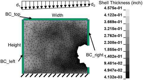
FIGURE 1. A typical corroded plate FE model of the bottom portion of a web or stiffener plate for a corroded steel girder.

TABLE 1

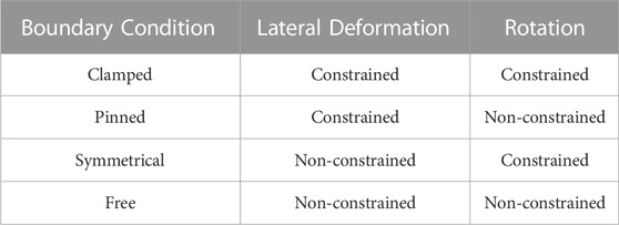
TABLE 1. Constrained degrees of freedom for the potential boundary conditions of the plate edges.

2.1 Generating the required parameters for the corroded plate models

Each corroded plate model is defined by a series of parameters. These parameters include a set of dimensions, parameters to define the four high-frequency components and one low-frequency component that make up the corroded surface, displacement parameters for the FE analysis, and boundary conditions for the plate edges. For each of these parameters, the distribution type and ranges are determined first. Once identified, 30,000 sets of parameters are randomly generated within the defined ranges and are used to generate the plate models.

2.1.1 Plate model dimensions

Each of the rectangular plate models is defined by a height (H), width (W), and intact thickness (t). The authors collected geometric data of corrosion damage from in-service steel bridge girders using 3D scanning (Hain et al., 2019), of which select results are shown in Figure 2. These field studies concluded that the width of the corroded region typically ranges from 4 to 10 inches, that the H:W ratio typically ranges from 1:2 to 2:1, and that the intact plate thickness, t, is typically between 1/16th and 1/8th of the plate width, W. To ensure that the training database for the neural networks is representative of known corrosion patterns, the plate width (W) for each model generated in this study is randomly selected from a uniform distribution spanning the range of 4–10 inches. The remaining height and intact thickness parameters can be determined from ln (H/W) and t/W, respectively, where ln (H/W) is the natural logarithm of H over W.

FIGURE 2

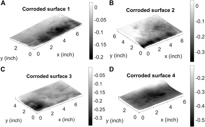
FIGURE 2. Four representative examples of corroded surface geometries from in-service steel bridge girders obtained from 3D scanning. (A–D) show the surface geometry of a corroded surface where the H:W ratio is approximately: (A) 1:2, (B) 1:1, (C) 1:1.75, (D) 1:1.5.

The H:W aspect ratio for common corrosion patterns ranges from 1:2 to 2:1. In lieu of more detailed data, it is assumed that a corroded region is equally likely to have a width greater than and less than the corrosion height. Therefore, the height parameter for each of the plate models, H, is calculated from the natural logarithm of H over W (ln (H/W)). The value of the natural logarithm is selected from a uniform distribution in the range of ln (1/2) to ln (2), i.e., −0.6931–0.6931, from which H can be determined. A uniform distribution is critical to ensure that the ratio of H:W is equally likely in the ranges of 1:2∼1:1 and 1:1∼2:1. The second parameter, t/W, is the ratio of intact plate thickness to plate width. Intact plate thickness is typically between 1/16th and 1/8th of the corroded plate width, W. For each of the plate models, the ratio t/W is randomly selected from a uniform distribution between 1/16 and 1/8 such that potential intact plate thickness values, t, are expected to span uniformly from W/16 to W/8. For example, for the minimum value of W, 4 inches, the range of H is 2–8 inches, and the range of t is 0.25–0.5 inches. For the maximum value of W, 10 inches, the range of H is 5–20 inches, and the range of t is 0.625–1.25 inches.

2.1.2 Corroded surface parameters

The irregularities of corrosion damage are included in each of the plate models used to build the training dataset by generating surfaces with intricate, irregular geometries. According to Zhang et al. (2023), the geometry of the corroded surface of a steel girder can be decomposed into four high-frequency components and one low-frequency component using Lanczos filters. Figure 3 demonstrates this process, where the original corroded surface along with the five frequency components are shown. The four high-frequency components represent the textures of different scales on the corroded surface, while the low-frequency component is representative of the overall shape of the corroded surface.

FIGURE 3

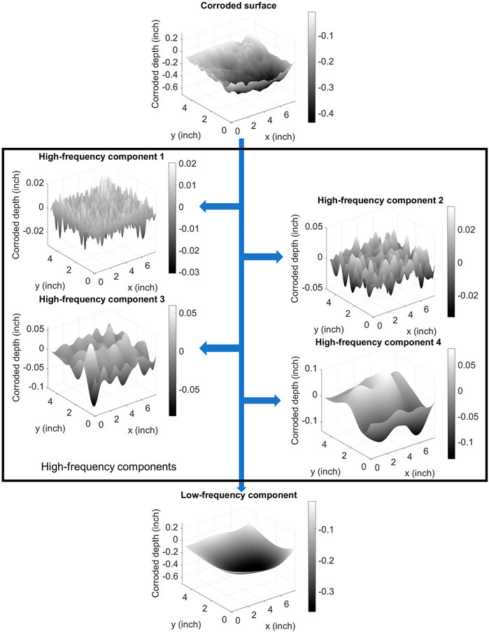
FIGURE 3. Decomposition of a corroded surface into four high-frequency components and one low-frequency component using Lanczos filters. The dimension of corroded depth is exaggerated in this figure for visualization purposes only.

Each of the high-frequency components is represented as a random field and is statistically characterized by its autocorrelation function, defined below in Eq. 1.

$R_{yy}\left(d\right)=E\left[\left(Y\left(x_1\right)-{\mu }_y\right)\left(Y\left(x_2\right)-{\mu }_y\right)\right]\mathrm{f}\mathrm{o}\mathrm{r}‖x_1-x_2‖=d(1)$

Here, x₁ and x₂ are any two points in the random field a distance d apart, Y (x₁) and Y (x₂) are the height values at points x₁ and x₂, and μ_y is the mean of the height values in the random field. Zhang et al. (2023) investigated the corrosion damage from in-service steel bridge girders and concluded that the autocorrelation function of the high-frequency component could be fit using the Hole-Gaussian function, shown below in Eq. 2.

$HG\left(d\right)={{\sigma }_h}^2\left(1-{\left(\frac{d}{l_c}\right)}^2\right)e^{-\frac{1}{2}{\left(\frac{d}{l_c}\right)}^2}(2)$

Here, σ_h is the standard deviation of the height values of the high-frequency component, and l_c is the correlation length of the high-frequency component. When d is equal to 0, the Hole-Gaussian function takes its largest value, σ_h², and is equal to the variance of the random field. This is consistent with Eq. 1, in which the calculated autocorrelation will be equal to the variance of the random field when x₁ and x₂ are the same point. When the value of d ranges from approximately l_c to 3l_c, the value of the Hole-Gaussian function is negative, forming peaks and valleys in the random field. The value of the Hole-Gaussian function is close to 0 for values of d beyond 3l_c since points in a random surface a large distance apart are independent of one another. The relationships between the two parameters, σ_h and l_c, and the cutoff frequency, f, of the Lanczos filter for the decomposition of a corroded surface are expressed in Eqs 3, 4.

${\sigma }_h=\left(1+v\right)\times \frac{6.297}{f}\times {10}^{-3}(3)$

$l_{\mathrm{c}}=\frac{0.283}{f}(4)$

The cutoff frequencies corresponding to the four high-frequency components used to generate the surface textures of the corroded plate models are 1.563 in⁻¹, 0.781 in⁻¹, 0.391 in⁻¹, and 0.195 in⁻¹, respectively. The variation parameter v in Eq. 3 follows a normal distribution with a mean of 0 and a standard deviation of 0.264 and reflects the varied magnitude of surface textures due to varying corrosion intensities.

The low-frequency component of a corroded surface was characterized and represented using a bivariate Lagrange polynomial surface constructed from a 4 × 4 two-dimensional Gauss point sample set from the low-frequency component. First, the low-frequency component was mapped to a square region with the range of −1 ≤ x ≤ 1 and −1 ≤ y ≤ 1. Second, the 4 × 4 Gauss point sample set is constructed based on the points where x = ±0.34 and ±0.86, and y = ±0.34 and ±0.86. The coordinates with the corroded depths of the 16 sample points can be represented as (x_i, y_j, z_ij), with i = 0, 1, 2, 3 and j = 0, 1, 2, 3. Finally, the low-frequency component is constructed from the Lagrange polynomial shown in Eq. 5. The Lagrange polynomial is the sum of a series of Lagrange bases, l_i,j (x, y), calculated from the set of 16 sample points. The Lagrange bases are determined from Eq. 6. It was verified that the constructed surface is close to the low-frequency component, with an average normalized root mean square error of less than 5% (Zhang et al., 2023).

$f\left(x,y\right)={\displaystyle \sum }_{0\le i\le \mathrm{3,0}\le j\le 3}{z}_{i,j}{l}_{i,j}\left(x,y\right)(5)$

$l_{i,j}\left(x,y\right)=\prod _{\begin{array}{c}0\le p\le 3\\ p\ne i\end{array}}\frac{x-x_p}{x_i-x_p}\prod _{\begin{array}{c}0\le q\le 3\\ q\ne j\end{array}}\frac{y-y_q}{y_j-y_q}\left(0\le i\le \mathrm{3,0}\le j\le 3\right)(6)$

In this research, artificial corroded surfaces for the plate models were generated based on the characterization method outlined above, with two corroded surfaces (one for each side) generated for each plate model. Each corroded surface is the summation of four high-frequency components and one low-frequency component. Each of the high-frequency components is generated as a random field using the Karhunen-Loeve (K-L) expansion method (Eq. 7) (Wang, 2008; Htun et al., 2013) and is based on the autocorrelation function from Eq. 1. To generate the corroded surfaces, σ_h and l_c must first be calculated according to Eqs 3, 4, respectively. The four cutoff frequencies, f, given above (1.563 in⁻¹, 0.781 in⁻¹, 0.391 in⁻¹, and 0.195 in⁻¹) are used. The variation parameter, v, shown in Eq. 3 is randomly generated for each plate model following a normal distribution with a mean of 0 and a standard deviation of 0.264. With ${\sigma }_h$ and $l_c$ known for each plate model, the covariance matrix of each high-frequency component can be generated. The covariance matrix is an N-by-N matrix, where N is the number of pixels in the high-frequency component. The elements in the covariance matrix, c_ij, are equal to the value of the autocorrelation function between points i and j and are calculated using the Hole-Gaussian function presented in Eq. 2. Finally, each high-frequency component, s, is generated from Eq. 7, where ξ is a set of uncorrelated random variables with zero mean and unit variance, and λ and φ are the eigenvalues and eigenvectors of the covariance matrix.

$\mathit{s}={\displaystyle \sum }_{\mathit{i}=\mathbf{1}}^{\mathit{N}}{\mathit{\xi }}_{\mathit{i}}\sqrt{{\mathit{\lambda }}_{\mathit{i}}}{\mathit{\phi }}_{\mathit{i}}(7)$

The low-frequency component for each of the corroded surfaces is generated as a bivariate Lagrange polynomial based on a 4 × 4 two-dimensional Gauss point sample set. Based on corrosion damage data collected by Hain et al., 2019, the corroded depth is defined in the range between 0 and 0.6 times the intact plate thickness, t. This range of allowable values for corroded depth is used to ensure that the generated FE models will account for varying corrosion intensities. Because the FE models will be used to train the neural networks, these machine learning models will have the ability to handle a wide range of corrosion intensities. To generate the low-frequency component, the corroded depth values at the 16 sample points are first randomly selected based on a uniform distribution in the range between 0 and 0.6t to consider a range of possible corrosion intensities. The low-frequency component is then constructed using Eqs 5, 6. Based on this definition, the low-frequency component will vary across the surface to produce a surface with variable corrosion damage.

After generating the high-frequency and low-frequency components, the corroded surface is calculated as the sum of all five components, which have the same dimensions as the plate. In summary, the parameters for generating a corroded surface consist of a single variation parameter v for the high-frequency components and 16 corroded depth ratios (depth/t) for the low-frequency component.

2.1.3 Displacement and boundary conditions

The trapezoidal distributed displacement applied to the top of the plate model, as shown in Figure 1, is characterized by the ratio between the displacements at the two ends, i.e., by d₁/d₂, and is considered constant during loading. Its logarithm form, ln (d₁/d₂), is selected from a uniform distribution in the range of ln (1/4) to ln (4), i.e., −1.3863–1.3863 such that the ratio of d₁:d₂ is expected to be equally likely within the ranges from 1:4 to 1:1 and from 1:1 to 4:1. The boundary conditions for the top (BC_top), left (BC_left), and right (BC_right) edges will be randomly generated. Since the plate models constructed can either be a stiffener plate or a web plate, the top boundary condition may be clamped, pinned, or symmetrical, and the left and right boundary conditions may be clamped, pinned, or free, depending on the possible locations of the plates at a girder end. Each of these options has the same probability (1/3) of being selected for each plate model. For the purposes of the training dataset constructed for this study, no restrictions were made on the combination of boundary conditions. The bottom edge of the plate models is always fixed due to the stiffness of the bottom flange.

In summary, a total of 41 parameters are required to generate each corroded plate model. Table 2 summarizes the necessary parameters, their selection distribution, and the selection range or options, as applicable. All parameters are considered independent of each other. A total of 30,000 sets of parameters are generated using a quasi-random number generator to ensure that the generated random samples uniformly cover the defined space (Kocis and Whiten, 1997; Joe and Kuo, 2003).

TABLE 2

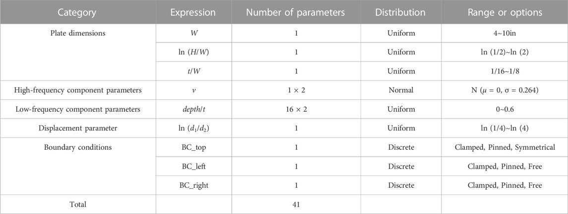
TABLE 2. Parameters required to generate each artificial corroded plate model.

2.2 Constructing FE models to calculate the compressive capacity of the corroded plate models

A total of 30,000 FE plate models are constructed from the 30,000 sets of quasi-randomly generated parameters created in Section 2.1; however, due to its irregularity and complexity, corrosion damage is challenging to incorporate accurately into FE models. To address this challenge, Zhang and Zaghi (2023) proposed an automated methodology for predicting the bearing capacity of corroded bridge girders using shell FE models that accurately represent the corrosion damage. The approach involves extracting geometric information from 3D point cloud data using Alpha shapes (Edelsbrunner et al., 1983) and the Douglas-Peucker algorithm (Douglas and Peucker, 1973) to detect and simplify the boundary of each plate, respectively. Delaunay triangulation (Ruppert, 1995; Shewchuk, 1996) is used to generate a triangular mesh for each plate member. Each node in the mesh is assigned unique thickness and eccentricity values, which are calculated based on the point cloud data, to capture the intricacies of the corrosion damage that would otherwise be lost in the model. To ensure the constructed FE model can accurately capture the corrosion damage while also ensuring an efficient FE analysis, the approach proposed three criteria to limit the size of each element in the FE mesh. First, the area (A) of the checked element should be less than k₁ times the cubic of the minimum nodal thicknesses (t_min) of the element, i.e., $A<k_1\times {t_{\min }}^3$. This ensures the element size is small enough in the regions with small remaining plate thickness. Second, the ratio of the maximum nodal thickness (t_max) to the minimum nodal thickness (t_min) of the checked element should be less than k₂, i.e., $\frac{t_{\max }}{t_{\min }}<k_2$. This criterion limits the element size in the regions with dramatic thickness change, where the stress is usually complex. Third, the relative error of the element thickness (t_ele) to the actual thickness (t_actual) at the centroid of the checked element should be less than k₃, i.e., $\frac{\left|t_{\mathrm{e}\mathrm{l}\mathrm{e}}-t_{actual}\right|}{t_{actual}}<k_3$. t_ele is calculated as the average of the three nodal thicknesses of the element, and t_actual is calculated from the point cloud data. This criterion ensures that the fluctuations in corroded surfaces are accurately captured in the mesh. The three parameters k₁, k₂, and k₃ are defined based on the extent of the corrosion damage and the resolution of the point cloud data. These three parameters determine the accuracy of the FE model. The smaller the parameter values, the more accurate the model, and the more time-consuming the FE analysis. To generate the mesh of the FE model, a relatively course mesh is generated first and all the elements are then checked against the three criteria. Any elements that violate any one of the three criteria are represented with smaller elements to refine the mesh. The accuracy of the FE models generated using this approach was validated by experimental results (Zhang and Zaghi, 2023).

This approach is used to construct the 30,000 FE models required for this research. Once the models are generated, FE analysis is used to evaluate the compressive capacity of the corroded plate models. LS-DYNA is used to analyze the generated FE models, as shown in Figure 1 (LSTC, 2018). The rotation and translation constraints are applied at the nodes on the edges based on the corresponding boundary conditions selected from Table 1. Due to the stiffness of the bottom flange, the bottom boundary condition of all plate models is fixed. The values of the parameters k₁, k₂, and k₃ are 50 in⁻¹, 1.5, and 5%, respectively, which are determined based on convergence analysis. The FE analysis results do not change obviously when the parameter values are further reduced.

Figure 4 shows a sample load-displacement curve resulting from a FE analysis for a typical plate model where the load is equal to the reaction force at the bottom (fixed) edge of the plate, and the displacement is measured at the middle of the top edge of the plate. The load-displacement curve is used to assess the compressive capacity of the corroded plate models; for example, the plate model used to generate the plot shown in Figure 4 has a compressive capacity of approximately 62 kips. The load-displacement curve captures the entire loading process of the plate model and reflects its mechanical characteristics, such as initial stiffness, failure capacity, and post-failure behavior. These characteristics are important for evaluating the strength of corroded plates; therefore, the load-displacement curve will be predicted using neural networks and will be compared to those generated by a FE analysis. As the purpose of this study is to evaluate the ability of neural networks to accurately predict the results of a rigorous FE analysis, the FE analysis was not calibrated against experimental data on the compressive capacity of corroded steel plates.

FIGURE 4

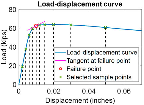
FIGURE 4. A sample load-displacement curve for a typical plate model.

2.3 Constructing the training data for neural network applications

The training data for the neural networks requires both an input and a corresponding output. The input data to the neural networks consists of the plate dimensions, remaining plate thickness, boundary conditions, and the displacement parameter, while the output data consists of the load-displacement curves obtained from the FE analysis. It is important to note that the input training data is of two data types: tabular and image. The tabular input data consists of two plate dimensions (H and W), three boundary conditions, and one displacement parameter (ln (d₁/d₂)). For the model training, the three boundary conditions are expanded into six constraints on edge degrees of freedom. On each edge, one boundary condition defines two constraints–one for lateral deformation and another for rotation, as shown in Table 1. The image data includes the thickness map and eccentricity map, which represent the remaining thickness and the eccentricity across the plate caused by asymmetric corrosion damage. Because the dimensions of the plate models fluctuate, the thickness and eccentricity maps vary in size from one plate model to the next. This is not convenient for training neural networks. Therefore, the thickness and eccentricity maps for all plate models are resized to 200 × 200 pixels for consistency. For example, the largest size of the plate models is 20 × 10 inches (H×W), which will have a remapped size of 10 × 20 points per inch. The lowest resolution occurs for the largest plate model and, therefore, the lowest resolution is 10 points per inch; this resolution is larger than twice the highest frequency of the generated corroded surfaces (1.563 inch^-1). Per the Nyquist theorem, the 200 × 200 feature map is sufficiently detailed to be able to capture the high-frequency components of the corroded surfaces (Por et al., 2019).

The output data, which is the data the neural network is trying to match, consists of the load-displacement curves obtained from the FE analysis shown in Figure 4. For the FE analysis, a fixed loading process defined by the acceleration applied at the top of the plate models is used. The acceleration starts from 0 to reduce the dynamic effect of the loading rate on the plate and to measure a reliable static load-displacement curve. To ensure that all the plates fail, the final displacement is set proportional to the plate height, and the analysis time is calculated based on the acceleration curve and the final displacement. Not only do the load-displacement curves obtained from FE analysis consist of many points, but the number of points varies for different plate models since the number of analysis steps is related to the plate size. Because neural networks require that the output be consistent, a load-displacement vector (s_failure, f_failure, f_0.2, f_0.4, f_0.6, f_0.8, f_1.2, f_1.5, f₂, f₃, f₅) is constructed to represent the load-displacement curve. In the vector, s_failure and f_failure are the displacement and load at the failure point, respectively. The failure point is defined as the point where the plate’s stiffness is equal to 1/10 of the initial stiffness, as shown by the red point in Figure 4. The variables f_0.2 to f₅ ($f_x$) are set equal to the load values corresponding to the displacements at $x\times s_{failure}$ and are shown by the nine green points in Figure 4. In this way, each vector representing the load-displacement curves has eleven elements, regardless of the initial number of points on the curve.

3 Preprocessing the training data and training the neural networks

Three types of neural networks, MLP, CNN, and hybrid MLP-CNN, are trained and evaluated on their ability to predict the compressive capacity of corroded steel plate models. Multilayer perceptron (MLP) and convolutional neural network (CNN) are two basic architectures of neural networks (O’Shea and Nash, 2015; Ramchoun et al., 2016). MLP networks require that the input data be in a tabular form, usually vectors. A MLP is typically constructed by connecting multiple fully connected layers using activation functions (Dongare et al., 2012). In theory, a MLP has the potential to model any nonlinear relationship given a sufficient number of layers and neurons. A CNN is a regularized version of a MLP designed specifically for analyzing image data. By replacing fully connected layers with convolutional layers, a CNN significantly reduces the number of parameters and is less prone to overfitting when processing image data. MLP and CNN are typically used to process monomodal data, such as pure tabular or pure image, respectively. However, the training data in this research contains both tabular and image data, which cannot be processed in a MLP or a CNN directly. Two strategies are used to address this problem. The first strategy consists of converting the multimodal data into monomodal data. For the MLP, numerical features such as the average remaining plate thickness can be manually extracted from the image data and appended to the tabular data, as will be discussed in Section 3.1.1. For the CNN, the relationship between the tabular data (plate dimensions) and the output data (failure load and failure displacement) can be estimated by simplifying and idealizing the FE models, as will be discussed in Section 3.1.2. The second strategy consists of using a hybrid MLP-CNN machine learning model. A hybrid MLP-CNN combines a MLP and a CNN where tabular and image data are fed to the MLP and CNN branches, respectively (Zhang et al., 2018; Ahsan et al., 2020). The outputs of the two branches are connected to predict the results through the subsequent fully connected layers. The following sections will focus on the methods used to preprocess the training data and to train the models for the three types of neural networks.

3.1 Data preprocessing

Before a neural network can be trained, the data must be properly formatted and organized. This is because different neural network architectures have been designed to handle different data structures. A MLP requires the training data to be solely in tabular form, while a CNN is designed to process only image data. The training data compiled for this research must therefore be preprocessed into a compatible format for each type of neural network before the networks can be trained. The following three sections will discuss the preprocessing steps required for the training dataset before the MLP, CNN, and hybrid MLP-CNN models can be trained, respectively.

3.1.1 Data preprocessing for MLP

A MLP neural network can only read tabular data. To use the images in the training data, three numerical features–average thickness, minimum thickness, and hole area ratio–are manually extracted from the thickness maps. These three features are commonly used to investigate the effect of corrosion damage on steel plate girders (Liu et al., 2011; Khurram et al., 2014a; Khurram et al., 2014b). The three features are then appended to the vector of the tabular data as the new input data. Their addition to the input vector allows the MLP neural network to account for the variable levels of corrosion in the FE plate models. For the output data, the load-displacement values are converted to logarithms, ln(s) and ln(f), in order to eliminate the error caused by the extensive range of output data and to convert the highly skewed distributed data to an approximately normal distribution. As depicted in Figure 5A, the distribution of the failure loads of the plate models is skewed to the right and the failure loads range from less than 10 kips to more than 350 kips. This skew in the data is removed by taking the logarithm of the failure loads and displacements, which yields the approximately normal distribution shown in Figure 5B. This is done to improve the accuracy of the trained neural networks (Zhang et al., 2017).

FIGURE 5

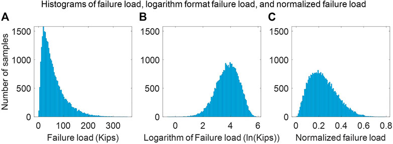
FIGURE 5. Histograms of failure load values with the number of bins as 100–(A) histogram of original failure load values, (B) histogram of the logarithm of failure load values, and (C) histogram of the normalized failure load values.

The Mean Squared Error (MSE) loss function is used for regression analysis during the training process for neural networks and is calculated based on the difference between the predicted and target results. For example, if during the training process the neural network predicts a failure load of 20 kips, but the plate has a known capacity of 10 kips from the FE analysis, then the prediction error is 10 kips. The same is true for a prediction of 360 kips when the failure load is known to be 350 kips. If the failure load value is selected as the output of the neural networks, these predictions are considered the same performance and have the same effect on the training process. However, the prediction of 20 kips corresponds to a 100% error for 10 kips, while 360 kips corresponds to a 2.9% error for 350 kips. They should be treated differently. Therefore, using absolute error to update the neural networks will lead to significant errors for the low-capacity samples. By converting the output data to logarithm form, the difference between the predicted and target results for the two cases in the above example will be $\ln \left(20\right)-\ln \left(10\right)\approx 0.693$ and $\ln \left(360\right)-\ln \left(350\right)\approx 0.028$. The error for the first case is approximately 25 times greater than that for the second one. Thus, the loss function for the first case has a greater impact on the neural network, which corresponds to the larger percent error for the first case.

3.1.2 Data preprocessing for CNN

A CNN requires that the input data be formatted as images. Tabular data, such as the dimensions and boundary conditions of the plate models, cannot be fed to the network directly. To consider dimensional data, the training data is normalized to remove the effects of varying plate dimensions from the input images and output vectors. For the input images, the values in the thickness and eccentricity maps can be divided by the intact thickness of the plates, t, to produce the thickness and eccentricity ratio maps. In addition, the thickness and eccentricity ratio maps ensure that the trained neural networks can account for the varying corrosion intensities included in the FE model training database. The output of the CNN is a vector representing the load-displacement curves of the FE models. To normalize the output data, the failure mode of the plate models is assumed as the yielding failure of a uniformly corroded plate such that the failure displacement is proportional to the plate height, H, and that the failure load is proportional to the cross-sectional area of the plate, W×t. The output displacements and loads contained in the output vector are divided by the plate height, H, and by the yielding capacity of the intact plate, W×t×f_y, respectively, where f_y = 50 ksi for all plates. In this way, all the training data is transformed such that dimensions are not involved in the training of the neural networks. Figure 5C shows a histogram of the normalized failure load ratio across all plate models, calculated as the failure load divided by the theoretical yielding failure load of the intact plate (W×t×f_y).

The boundary conditions of the plate models should be considered in the input data to train as accurate a model as possible. To accomplish this, the boundary conditions of the plates are utilized to produce 2D maps of the theoretical buckling shapes. Figure 6 shows two examples of the theoretical buckling shapes of plate models with different boundary conditions in both 2D and 3D. Figures 6A, B are the 2D representations of the 3D buckling shapes shown in Figures 6C, D, respectively. The 2D model is representative of the heatmap fed to the CNNs, whereas the 3D model is included for visualization purposes. Because a CNN requires that all input images be of the same size, the buckling shapes are also sized at 200 × 200 pixels. Finally, all input layers–thickness ratio map, eccentricity ratio map, and theoretical buckling shape–are stacked into one 3D array that can be fed to the CNN for training.

FIGURE 6

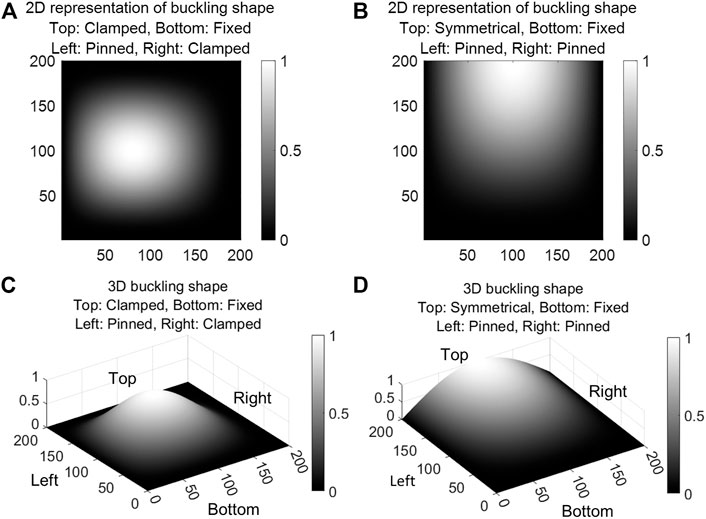
FIGURE 6. Typical buckling shapes of the FE plate models. -(A) and (C): 2D and 3D representations, respectively, of the theoretical buckling shape of a plate with the top and right edges clamped, the left edge pinned, and the bottom edge fixed. -(B) and (D): 2D and 3D representations, respectively, of the theoretical buckling shape of a plate with the top boundary condition symmetrical, the right and left edges pinned, and the bottom edge fixed.

3.1.3 Data preprocessing for hybrid MLP-CNN

The input data to a hybrid MLP-CNN model should be both tabular and image data. The tabular data is fed to the MLP branch while the image data is fed to the CNN branch. Therefore, there is no need for feature extraction or data type conversion for the hybrid MLP-CNN model. Similar to the dataset for the MLP network, the load-displacement values in the output data are represented in logarithm format to eliminate the errors caused by the extensively ranged and highly skewed training data. In the hybrid MLP-CNN model, the plate dimensions, boundary conditions, and displacement parameter are input directly to the MLP branch. Similarly, the thickness and eccentricity maps are input directly to the CNN branch without additional preprocessing. For the hybrid model, the MLP branch handles the effect of the tabular data, such as plate dimensions, whereas the CNN branch handles the effect of varying corrosion levels from one plate model to another.

Table 3 provides a summary of the preprocessed input and output data types required for the training of the three neural network architectures evaluated in this study.

TABLE 3

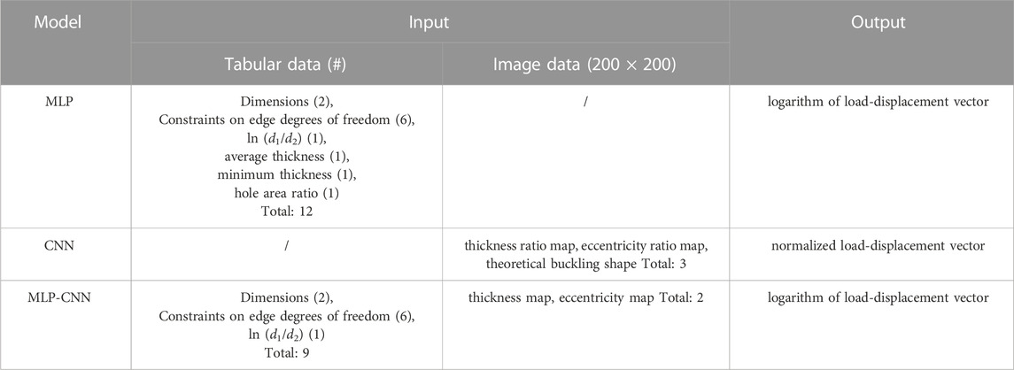
TABLE 3. Input and output of neural network models.

3.1.4 Statistical analysis on training data

Before training the neural networks, statistical analyses are performed on the training data, including an evaluation of the statistical distribution of the training data and the correlation between the input and output data.

The statistical distributions of the tabular parameters are investigated. In the tabular parameters, the plate width (W), boundary conditions, and the displacement parameter (ln (d₁/d₂)) were generated based on the defined distributions summarized in Section 2.1. The plate height, H, was generated from W and ln (H/W). The distribution of H is shown in Figure 7A. Within the training dataset, H ranges from 2 to 20 inches and has a mean of 7.53 inches and a standard deviation of 3.59 inches. The distributions of the three parameters extracted from the image data are shown in Figures 7B–D. The average thickness of the corroded plate models has a mean of 0.284 inches and a standard deviation of 0.122 inches. The minimum thickness and the hole area ratio are mutually exclusive, which means that a sample with a non-zero minimum thickness will have a hole area ratio of 0, and vice versa. For the training data, the number of samples with a non-zero minimum thickness is 19,488, and the number of samples with a non-zero hole area ratio is 10,512. Figures 7C, D only include the samples with non-zero minimum thickness and non-zero hole area ratio, respectively. Both of these two distributions are highly skewed to the right. The minimum thickness has a mean of 0.073 inch and a standard deviation of 0.063 inch. The maximum value of the minimum thickness is 0.489 inch. The hole area ratio has a mean of 0.023 and a standard deviation of 0.028. The maximum hole area ratio is 0.199.

FIGURE 7

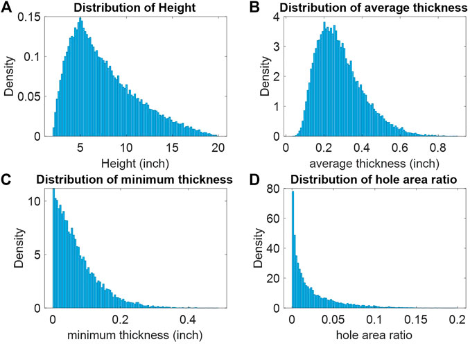
FIGURE 7. Statistical distributions of tabular input data. (A) Histogram of plate heights, H, contained in the training dataset, (B) Histogram of the average plate thicknesses contained in the training dataset, (C) Histogram of the minimum plate thicknesses contained in the training dataset, (D) Histogram of the hole-area ratios contained in the training dataset.

The linear correlation between the tabular input data and the failure load and displacement values is investigated. The linear correlation is calculated by the Pearson correlation coefficient, defined below in Eq. 8. The results of these calculations are listed in Table 4. It is noted that the nonlinear correlation between parameters is not investigated here, as the analysis was performed only to investigate which parameters showed correlation with the output data.

${\mathit{r}}_{\mathit{x}\mathit{y}}=\frac{{\sum }_{\mathit{i}=\mathbf{1}}^{\mathit{n}}\left({\mathit{x}}_{\mathit{i}}-\overline{\mathit{x}}\right)\left({\mathit{y}}_{\mathit{i}}-\overline{\mathit{y}}\right)}{\sqrt{{\sum }_{\mathit{i}=\mathbf{1}}^{\mathit{n}}{\left({\mathit{x}}_{\mathit{i}}-\overline{\mathit{x}}\right)}^{\mathbf{2}}}\sqrt{{\sum }_{\mathit{i}=\mathbf{1}}^{\mathit{n}}{\left({\mathit{y}}_{\mathit{i}}-\overline{\mathit{y}}\right)}^{\mathbf{2}}}}(8)$

TABLE 4

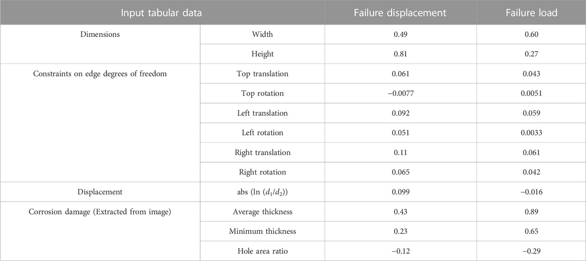
TABLE 4. Correlation between the tabular data and the failure load and displacement values.

Here, n is the sample size (30,000); x_i and y_i are the individual sample values; $\overline{x}$ and $\overline{y}$ are the sample means. The relationships between the tabular input data (x) and the output data (y) can be found from the correlation coefficients. First, the dimensions have a strong correlation with the output data. Specifically, the width is more related to the failure load with a correlation value of 0.6, while the height is more related to the failure displacement with a correlation value of 0.81. Second, two of the three manually extracted features (average thickness and minimum thickness) for the MLP show a high correlation with the output data, especially with the failure load. The correlation values between these two features and the failure load are 0.89 and 0.65, respectively. The high correlation values mean that the manually extracted features are critical to predicting the failure load and displacement. Further, the correlation value between the hole area ratio and the failure load is −0.29. This value is negative, which means that as the hole area ratio increases, the compressive capacity of the plate decreases. Finally, the correlation values between boundary conditions and the output data are less than 0.15. It is found that most of the corroded plates failed due to local failure rather than global buckling because of the varied thickness across each corroded plate. The boundary conditions and displacement slope have minimum effects on the local failures inside the plates.

3.2 Training models

Before the neural networks are trained, the training data is split into three categories–training, validation, and test–using an 85%/10%/5% split. The typical architectures of the MLP, CNN, and hybrid MLP-CNN are shown in Figure 8. The MLP neural network (Figure 8A) is constructed by connecting multiple fully connected layers using activation functions. For example, a single layer in a MLP can be expressed as y = f (Wx + b), where x is the input vector of the layer, y is the output vector, W is the weight matrix, b is the bias vector, and f () is the nonlinear activation function. The fully connected layer, Wx + b, integrates all input data for predicting the values to the next layer, while the activation function, f (), introduces nonlinearity to the neural network. By convention, the activation function is not applied at the last layer for a regression task (Goodfellow et al., 2016), as shown in the figures. The parameters in the MLP consist of the weight matrix, W, and bias vector, b, in each layer. In the CNN (Figure 8B), convolutional layers are used to extract features from the input image. The following fully connected layers combine all the extracted features for prediction. The activation function, f (), is applied to each convolutional and fully connected layer, except the last one. The parameters in the CNN consist of the kernel tensor, K, and bias vector, h, in each convolutional layer and the weight matrix, W, and bias vector, b, in each fully connected layer. For the hybrid MLP-CNN (Figure 8C), the outputs of the MLP and CNN branches are connected and followed by fully connected layers, which combine the outputs to predict the results. The parameters in the hybrid MLP-CNN model consist of the parameters in the MLP and CNN branches and the weights and biases in the joint layers.

FIGURE 8

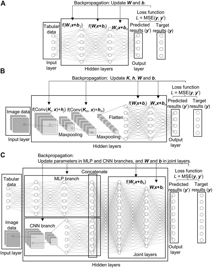
FIGURE 8. Typical architecture of the three neural networks–(A) MLP, (B) CNN, and (C) hybrid MLP-CNN.

For all three neural networks, a mean squared error (MSE) function (Eq. 9) is selected to calculate the loss values for solving regression problems. In the equation, y and y’ are the target result and the predicted result from the neural networks, respectively. The loss values represent the closeness between the predicted and target results. During the training process, the loss value of the training data is calculated in each iteration. Once the loss values have been calculated, the Adam optimizer is used to update all parameters in the neural networks to minimize the loss value. In addition, the loss value of the validation data is calculated every 50 iterations and is recorded to monitor the generalization of the trained neural network, i.e., how well the neural network performs when making predictions on data not contained in the training dataset. The training process terminated once the current validation loss was larger than the previously smallest validation loss 20 times. The hyperparameters of the three neural networks are determined through random search fine-tuning as follows. A set of options for the hyperparameters are predefined first. The predefined options for the number of layers for the MLP model and the MLP branch in the hybrid MLP-CNN model are {2, 3, 4}. Similarly, the number of layers for the CNN model and the CNN branch in the hybrid MLP-CNN model can be selected from the set {3, 4, 5, 6}. The maximum numbers of neurons for the MLP model and the MLP branch are selected from {16, 32, 64, 128}. The maximum number of channels for the CNN model and the CNN branch are selected from {32, 64, 128, 256}. The options for batch size are {64, 128, 256, 512}, and the options for learning rate are {1e-2, 1e-3, 1e-4, 1e-5}. The hyperparameters are randomly sampled from the predefined options, and the model is trained and evaluated with these hyperparameters. The options of the hyperparameters are then reduced based on the loss value of the validation data. The process is repeated several times, and the best set of hyperparameters is selected. Based on Occam’s razor principle, the simplest model is selected when the performances are close (Bargagli Stoffi et al., 2022). The final architectures of the models for the three types of neural networks are shown in Table 5. The MLP model has two hidden layers with 64 neurons in each layer. The CNN model has four convolutional layers followed by three fully connected layers. The sizes of all the convolutional kernels are 3 × 3. The numbers of channels for the four convolutional layers are 8, 16, 32, and 64, respectively. A 2 × 2 maxpooling layer follows each convolutional layer to down sample the image size. The numbers of neurons for the three fully connected layers are 1,024, 256, and 32, respectively. The CNN branch of the hybrid MLP-CNN model has the same architecture as the CNN model, and the MLP branch has two layers, with 16 neurons in the first layer and 32 neurons in the second layer. The output vectors of the MLP and CNN branches are concatenated and are followed by three layers of fully connected layers to predict the results. For all three models, the activation function is selected as the Rectified Linear Unit (ReLU) function, f(x) = max (0, x). The finalized batch size is 256, and the learning rate is 1e-3.

$MSE=\frac{1}{n}\sum {\left(y-y^{\prime }\right)}^2(9)$

TABLE 5

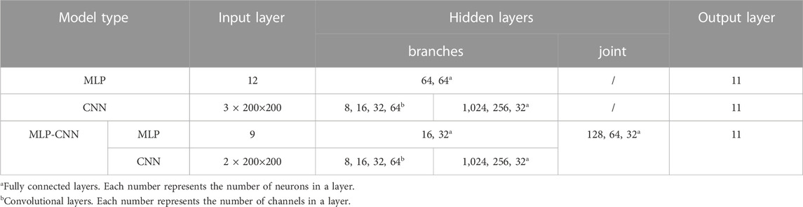
TABLE 5. Architectures of the three trained neural network models.

4 Results analysis

The mean absolute percentage error (MAPE, Eq. 10) is adopted to evaluate the performance of the three neural networks. The MAPE of s_failure and f_failure, and the average MAPE of the eleven outputs corresponding to points on the load-displacement curve for the three networks are calculated separately on both the training and test data and are listed in Table 6.

$\mathrm{M}\mathrm{A}\mathrm{P}\mathrm{E}=\frac{1}{n}{\displaystyle \sum }_{t=1}^n\left|\frac{A_t-F_t}{A_t}\right|\times 100\%(10)$

TABLE 6

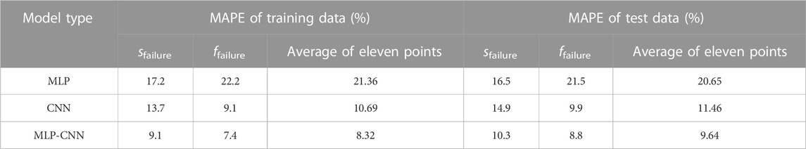
TABLE 6. MAPE of the outputs of training and test data for the three trained neural networks.

The MAPE values of the training data are close to (MLP) or slightly smaller than (CNN and hybrid MLP-CNN) that of the test data. The average MAPE values of the eleven points in the load-displacement vector for the training data range from 21.36% for the MLP model to 10.69% and 8.32% for the CNN and hybrid MLP-CNN models, respectively. Similarly, the average MAPE values for the load-displacement vector on the test data range from 20.65% for the MLP model to 11.46% and 9.64% for the CNN and hybrid MLP-CNN models, respectively. The MAPE values are found to be consistent across the training and test datasets, which signifies that there is no obvious overfitting in the neural networks. These error percentages are significantly better than the accuracy known for simplified methods that consider corrosion damage as uniform section loss, which can be up to 100% (Tzortzinis et al., 2021a; Hain et al., 2021). This demonstrates that the neural-network-based models are capable of predicting the results of a rigorous FE analysis and are able to estimate the residual load-carrying capacity of a corroded plate.

The hybrid MLP-CNN model consistently involves less error when compared to the MLP and CNN models, which means that the hybrid MLP-CNN model performs better than the standalone MLP and CNN models for predicting the compressive capacity of corroded plates. This is likely due to the fact that the hybrid MLP-CNN model does not require additional preprocessing of the training data, such as manually extracting features from image data or removing dimensions from the input and output data. These processes simplify the data, but also sacrifice some information contained in the data. For example, to involve the image data for predicting the compressive capacity of the corroded plate models in the training of the MLP model, three numerical features–average thickness, minimum thickness, and hole area ratio–are manually extracted from thickness maps and fed to the model. Although the manually extracted features and the load and displacement values are strongly correlated (Table 4), the MLP model has much larger errors than the CNN and the hybrid MLP-CNN models. The manually extracted features may disregard information that is important for accurately predicting the results. For example, the manually extracted features ignore the variations in the thickness across the corroded plates. Of note, the improved performance of the CNN when compared to the MLP confirms that the CNN model can extract critical features from image data required for the accurate prediction of the compressive capacity of corroded steel plates.

Figure 9 depicts four plots which each compare the load-displacement curves obtained from the FE analysis to those obtained from each of the three neural network models. The displayed plots are randomly selected samples from the test dataset, so the neural networks have not been exposed to these plate models during the training process. The solid black curves display the load-displacement curves obtained from the FE analysis. Figures 9A, C, D are consistent with the calculated MAPE in Table 6, in which the MLP model has more error than the CNN and hybrid MLP-CNN models. From Table 6, it is also noted that the CNN and hybrid MLP-CNN models have similar errors, which is confirmed by the plots in Figure 9.

FIGURE 9

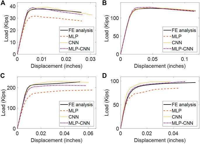
FIGURE 9. Comparison of the load-displacement curves predicted by the neural networks with the target load-displacement curves obtained from FE analysis. (A–D) show load-displacement curves produced for four different test plate FE models with varying expected failure loads of approximately: (A) 35 kips, (B) 125 kips, (C) 215 kips, (D) 85 kips.

Furthermore, the prediction process using neural network models is extremely fast compared to traditional FE analysis. For example, the time required to predict the capacity of a corroded plate using the neural network models, from inputting the parameters to obtaining the results, is less that 1 minute. In contrast, constructing and analyzing a FE model with accurate corrosion damage representation for prediction takes around 10 minutes if the automatic FE model construction method (Zhang and Zaghi, 2023) is used. This time savings can increase significantly when the methods are applied to a larger model, such as a corroded bridge girder.

5 Summary and conclusion

This research evaluated the feasibility of using neural networks to predict the compressive capacity of steel plate FE models. The capability of three neural network architectures (MLP, CNN, and hybrid MLP-CNN) to accurately predict the known capacity of a corroded steel plate was evaluated. The dataset used to train the neural network models consisted of 30,000 FE plate models and the corresponding load-displacement curves obtained from the FE analysis. The MLP model is trained using tabular input data only. In addition to plate dimensions, edge degree-of-freedom constraints, and a displacement parameter, the corrosion damage was represented by three parameters including average remaining plate thickness, minimum remaining plate thickness, and a hole area ratio. For the CNN model, plate dimensions were incorporated into the training data by producing thickness and eccentricity ratio maps. In addition, constraints on edge degree-of-freedoms were represented by the theoretical buckling shapes. Finally, the hybrid MLP-CNN model could accept both tabular and image data. Therefore, plate dimensions, edge degree-of-freedom constraints, and the displacement parameter were fed directly to the MLP branch, while image data including thickness and eccentricity maps were fed to the CNN branch. Each of the trained networks was evaluated on its ability to accurately predict the load-displacement curve originally obtained through a rigorous FE analysis for a test dataset. This test dataset was 5% of the total training dataset and was not used during the training process.

The evaluation of the three models illustrated that neural networks are capable of predicting the results of a rigorous FE analysis. Of the three architectures evaluated, the MLP model had the largest MAPE on both the training and test datasets. The CNN and the hybrid MLP-CNN models both performed better than the MLP model, with MAPE values as low as 8%–10% on both the training and test datasets for the hybrid MLP-CNN model. These results suggest that, once trained on a representative dataset, a hybrid MLP-CNN model can be used to accurately estimate the load-carrying capacity of a corroded steel plate. A fully trained model therefore has the potential to remove the requirement of FE analysis for future predictions. Furthermore, the reduced MAPE of the CNN and hybrid MLP-CNN models compared to the MLP model demonstrate the importance of representing the intricacies of corrosion damage with images rather than a set of single-valued parameters. A large proportion of model accuracy is therefore likely to be driven by the intricacies of corrosion damage which cannot be sufficiently represented by single-valued parameters or by broad model simplifications, such as a uniform remaining thickness.

Whereas this study focused on evaluating the feasibility of using neural networks to accurately predict the load-displacement behavior of corroded steel plates, the evaluation presented in the current study is limited by the dataset used to train the models. The accuracy of the model predictions is constrained by the range of plate dimensions, edge boundary conditions, etc., included in the training dataset. These ranges reflect typical scenarios of corrosion damage in steel bridge girders, but they may not encompass all possible scenarios. If the parameters of a plate fall outside of these ranges, the accuracy of the results obtained from the neural networks trained on the generated plate models may be compromised. Further, the proposed models have not been evaluated on their ability to predict experimentally collected load-displacement behaviors of corroded steel plates.

Future research should focus on evaluating the accuracy of the proposed model on experimental data. Corroded steel plates within the geometric constraints of the dataset should be compression tested and the experimental load-displacement curves compared with those predicted by the FE models and the trained neural networks. Future research should also investigate the ability of neural networks to predict the residual bearing capacity of corroded steel bridge girders. A training dataset can be constructed on FE models of corroded steel girders and used to train a neural network in a manner similar to that presented in this study. Once experimentally validated, a trained neural network may be used by practicing structural engineers to accurately evaluate the residual bearing capacity of in-service steel girders. This information can then be used to guide the allocation of funding for bridge repair and rehabilitation projects. In conclusion, neural networks have the ability to accurately predict the outcome of a rigorous FE analysis and, if experimentally validated, neural networks may be used to estimate the capacities of in-service members.

Data availability statement

The raw data supporting the conclusion of this article will be made available by the authors, without undue reservation.

Author contributions

AZ contributed to conception of the study and supervised the overall research work. TZ created the database, developed the models, and wrote the draft of the manuscript. MV wrote sections of the manuscript and revised the manuscript. All authors have made a substantial, direct, and intellectual contribution to the work, and approved the submitted version.

Funding

This work was supported by a funding (SPR-2310) from the Connecticut Department of Transportation.

Conflict of interest

The authors declare that the research was conducted in the absence of any commercial or financial relationships that could be construed as a potential conflict of interest.

Publisher’s note

All claims expressed in this article are solely those of the authors and do not necessarily represent those of their affiliated organizations, or those of the publisher, the editors and the reviewers. Any product that may be evaluated in this article, or claim that may be made by its manufacturer, is not guaranteed or endorsed by the publisher.

References

Ahsan, M. M., Alam, T. E., Trafalis, T., and Huebner, P. (2020). Deep MLP-CNN model using mixed-data to distinguish between COVID-19 and Non-COVID-19 patients. Symmetry 12 (9), 1526. doi:10.3390/sym12091526

CrossRef Full Text | Google Scholar

Albawi, S., Mohammed, T. A., and Al-Zawi, S. (2018). “Understanding of a convolutional neural network.” in Proceedings of 2017 international conference on engineering and Technology, ICET 2017, IEEE, 1–6.

Google Scholar

ASCE (2021). 2021 Infrastructure report card.

Google Scholar

ASTM (2021). Standard test methods and definitions for mechanical testing of steel products. West Conshohocken, PA.

Google Scholar

Bargagli Stoffi, F. J., Cevolani, G., and Gnecco, G. (2022). Simple models in complex worlds: Occam’s razor and statistical learning theory.” Minds and machines. Springer Neth. 32 (1), 13–42. doi:10.1007/s11023-022-09592-z

CrossRef Full Text | Google Scholar

Carleo, G., Cirac, I., Cranmer, K., Daudet, L., Schuld, M., Tishby, N., et al. (2019). Machine learning and the physical sciences. Rev. Mod. Phys. Am. Phys. Soc. 91 (4), 045002. doi:10.1103/revmodphys.91.045002

CrossRef Full Text | Google Scholar

Daniel, , Cenggoro, T. W., and Pardamean, B. (2023). A systematic literature review of machine learning application in COVID-19 medical image classification. Procedia Comput. Sci. 216, 749–756.

PubMed Abstract | CrossRef Full Text | Google Scholar

Dongare, A. D., Kharde, R. R., and Kachare, A. D. (2012). Introduction to artificial neural network (ANN) methods. Int. J. Eng. Innovative Technol. (IJEIT) 2 (1), 189–194.

Google Scholar

Douglas, D. H., and Peucker, T. K. (1973). Algorithms for the reduction of the number of points required to represent a digitized line or its caricature. Can. Cartogr. 10 (2), 112–122. doi:10.3138/fm57-6770-u75u-7727

CrossRef Full Text | Google Scholar

Edelsbrunner, H., Kirkpatrick, D. G., and Seidel, R. (1983). On the shape of a set of points in the plane. IEEE Trans. Inf. Theory 29 (4), 551–559. doi:10.1109/tit.1983.1056714

CrossRef Full Text | Google Scholar

Goodfellow, I., Bengio, Y., and Courville, A. (2016). Deep learning. MIT press.

Google Scholar

Graciano, C., Kurtoglu, A. E., and Casanova, E. (2021). Machine learning approach for predicting the patch load resistance of slender austenitic stainless steel girders. Structures 30, 198–205. doi:10.1016/j.istruc.2021.01.012

CrossRef Full Text | Google Scholar

Hain, A., Zaghi, A. E., Kamali, A., Zaffetti, R. P., Overturf, B., and Pereira, F. E. (2019). Applicability of 3-D scanning Technology for section loss assessment in corroded steel beams. Transp. Res. Rec. 2673 (3), 271–280. doi:10.1177/0361198119832887

CrossRef Full Text | Google Scholar

Hain, A., Zhang, T., and Zaghi, A. E. (2021). “Estimation of the residual bearing capacity of corrosion damaged bridge beams using 3D scanning and finite element analysis,” in Bridge maintenance, safety, management, life-cycle sustainability and innovations, 3806–3813. doi:10.1201/9780429279119-519

CrossRef Full Text | Google Scholar

Htun, M. M., Kawamura, Y., and Ajiki, M. (2013). “A study on random field model for representation of corroded surface.” in Analysis and design of marine structures - proceedings of the 4th international conference on marine structures, MARSTRUCT 2013, 545–553.

CrossRef Full Text | Google Scholar

Joe, S., and Kuo, F. Y. (2003). Remark on Algorithm 659: Implementing Sobol’s quasirandom sequence generator. ACM Trans. Math. Softw. 29 (1), 49–57. doi:10.1145/641876.641879

CrossRef Full Text | Google Scholar

Kayser, J. R., and Nowak, A. S. (1989). Capacity loss due to corrosion in steel-girder bridges. J. Struct. Eng. 115 (6), 1525–1537. doi:10.1061/(asce)0733-9445(1989)115:6(1525)

CrossRef Full Text | Google Scholar

Khurram, N., Sasaki, E., Katsuchi, H., and Yamada, H. (2014a). Experimental and numerical evaluation of bearing capacity of steel plate girder affected by end panel corrosion. Int. J. Steel Struct. 14 (3), 659–676. doi:10.1007/s13296-014-3023-8

CrossRef Full Text | Google Scholar

Khurram, N., Sasaki, E., Kihira, H., Katsuchi, H., and Yamada, H. (2014b). Analytical demonstrations to assess residual bearing capacities of steel plate girder ends with stiffeners damaged by corrosion. Struct. Infrastructure Eng. 10 (1), 69–79. doi:10.1080/15732479.2012.697904

CrossRef Full Text | Google Scholar

Kocis, L., and Whiten, W. J. (1997). Computational investigations of low-discrepancy sequences. ACM Trans. Math. Softw. 23 (2), 266–294. doi:10.1145/264029.264064

CrossRef Full Text | Google Scholar

Liakos, K. G., Busato, P., Moshou, D., Pearson, S., and Bochtis, D. (2018). Machine learning in agriculture: A review. Sensors Switz. 18 (8), 2674. doi:10.3390/s18082674

PubMed Abstract | CrossRef Full Text | Google Scholar

Liu, C., Miyashita, T., and Nagai, M. (2011). Analytical study on shear capacity of steel I-girders with local corrosion nearby supports. Procedia Eng. 14, 2276–2284. doi:10.1016/j.proeng.2011.07.287

CrossRef Full Text | Google Scholar

LSTC (2018). LS-DYNA keyword user’s manual.

Google Scholar

Malekjafarian, A., Golpayegani, F., Moloney, C., and Clarke, S. (2019). A machine learning approach to bridge-damage detection using responses measured on a passing vehicle. Sensors Switz. 19 (18), 4035. doi:10.3390/s19184035

PubMed Abstract | CrossRef Full Text | Google Scholar

Mangalathu, S., Hwang, S. H., Choi, E., and Jeon, J. S. (2019). Rapid seismic damage evaluation of bridge portfolios using machine learning techniques. Eng. Struct. 201, 109785.

CrossRef Full Text | Google Scholar

McMullen, K. F., and Zaghi, A. E. (2020). Experimental evaluation of full-scale corroded steel plate girders repaired with UHPC. J. Bridge Eng. 25 (4), 1–13. doi:10.1061/(asce)be.1943-5592.0001535

CrossRef Full Text | Google Scholar

O’Shea, K., and Nash, R. (2015). An introduction to convolutional neural networks, 1–11.

Google Scholar

Por, E., Kooten, M. V., and Sarkovic, V. (2019). Nyquist–Shannon sampling theorem. Leiden, Netherlands: Leiden University, 1–4.

Google Scholar

Ramchoun, H., Amine, M., Idrissi, J., Ghanou, Y., and Ettaouil, M. (2016). Multilayer perceptron: Architecture optimization and training. Int. J. Interact. Multimedia Artif. Intell. 4 (1), 26. doi:10.9781/ijimai.2016.415

CrossRef Full Text | Google Scholar

Ruder, S. (2016). An overview of gradient descent optimization algorithms, 1–14.

Google Scholar

Ruppert, J. (1995). A delaunay refinement algorithm for quality 2-dimensional mesh generation. J. Algorithms 18 (3), 548–585. doi:10.1006/jagm.1995.1021

CrossRef Full Text | Google Scholar

Sarker, I. H. (2021). Machine learning: Algorithms, real-world applications and research directions. SN Comput. Sci. 2 (3), 1–21. doi:10.1007/s42979-021-00592-x

CrossRef Full Text | Google Scholar

Shewchuk, J. R. (1996). “Triangle: Engineering a 2D quality mesh generator and delaunay triangulator,” in Lecture notes in computer science (including subseries lecture notes in artificial intelligence and lecture notes in bioinformatics), 1148, 203–222.

CrossRef Full Text | Google Scholar

Tzortzinis, G., Ai, C., Breña, S. F., and Gerasimidis, S. (2022). Using 3D laser scanning for estimating the capacity of corroded steel bridge girders: Experiments, computations and analytical solutions. Eng. Struct. 265, 114407. doi:10.1016/j.engstruct.2022.114407

CrossRef Full Text | Google Scholar

Tzortzinis, G., Knickle, B. T., Bardow, A., Breña, S. F., and Gerasimidis, S. (2021a). Strength evaluation of deteriorated girder ends. I: Experimental study on naturally corroded I-beams. Thin-Walled Struct. 159, 107220. doi:10.1016/j.tws.2020.107220

CrossRef Full Text | Google Scholar

Tzortzinis, G., Knickle, B. T., Bardow, A., Breña, S. F., and Gerasimidis, S. (2021b). Strength evaluation of deteriorated girder ends. II: Numerical study on corroded I-beams. Thin-Walled Struct. 159, 107216. doi:10.1016/j.tws.2020.107216

CrossRef Full Text | Google Scholar

Wakjira, T. G., Rahmzadeh, A., Alam, M. S., and Tremblay, R. (2022). Explainable machine learning based efficient prediction tool for lateral cyclic response of post-tensioned base rocking steel bridge piers. Structures 44, 947–964. doi:10.1016/j.istruc.2022.08.023

CrossRef Full Text | Google Scholar

Wang, L. (2008). Karhunen-Loeve expansions and their applications. London, United Kingdom: The London School of Economics and Political Science.

Google Scholar

Xu, Y., Zheng, B., and Zhang, M. (2021). Capacity prediction of cold-formed stainless steel tubular columns using machine learning methods. J. Constr. Steel Res. 182, 106682. doi:10.1016/j.jcsr.2021.106682

CrossRef Full Text | Google Scholar

Zhang, C., Pan, X., Li, H., Gardiner, A., Sargent, I., Hare, J., et al. (2018). A hybrid MLP-CNN classifier for very fine resolution remotely sensed image classification. ISPRS J. Photogrammetry Remote Sens. 140, 133–144. doi:10.1016/j.isprsjprs.2017.07.014

CrossRef Full Text | Google Scholar

Zhang, T., Zaghi, A. E., and Bagtzoglou, A. C. (2023). Geometric characterization of localized corroded surfaces in steel bridge girders. Manuscript in preparation.

Google Scholar

Zhang, T., and Zaghi, A. E. (2023). Estimation of the residual bearing strength of corroded bridge girders using 3D scan data. Manuscript submitted for publication.

Google Scholar

Zhang, X., Fang, Z., Wen, Y., Li, Z., and Qiao, Y. (2017). “Range loss for deep face recognition with long-tailed training data.” in Proceedings of the IEEE international conference on computer vision, 5419–5428.

CrossRef Full Text | Google Scholar