A graph-based explanatory model for room-based energy efficiency analysis based on BIM data

1 Introduction

The global energy consumption rate has experienced a significant increase over the past decade, reflecting the growing demand for energy resources. This is not good news leading to sustainability and fighting climate change. The building sector accounts for over 40% of global energy consumption, as reported in 2022 (Saini et al., 2022). Energy consumption in buildings is projected to increase by an average of 1.3% per year from 2018 to 2050 in OECD countries, including the United States, Canada, Europe, and Australia. Non-OECD countries, such as the Middle East, China, and Russia, are expected to experience a higher annual increase of over 2% in energy consumption. On the other hand, climate change is an emerging issue that needs to be considered and makes our buildings more resilient and sustainable to heat loss and ener15.6 GB waste (Teske et al., 2018; Ahmad and Zhang, 2020).

To deal with these concerns, recent research on new building development projects focused on seeking novel ways to design and retrofit the buildings more energy-efficiently. To do so, the interest in using newly available datasets such as Building Information Modelling (BIM) and applying data-driven solutions emerge as the efficient and suitable option for the Building Energy Consumption Estimation (BECE) analysis rather than employing classical physics-based models (Li et al., 2010) to improve the estimation and prediction of building energy consumption in different stages of design, development, and retrofitting.

Data-driven-based BECE requires detailed static and dynamic data to simulate building energy consumption, eventually leading to prediction learning from historical/available data. Data-driven energy consumption prediction has been a prominent area of research in recent years. Numerous review studies have been conducted to analyze and evaluate existing data-driven approaches. These studies contribute to advancing knowledge and informing the building industry, for example, categorizing building energy consumption prediction methods into several categories, including elaborate engineering methods, simplified engineering methods, statistical methods, Artificial Neural Network (ANN)-based methods, Support Vector Machine (SVM)-based methods, and grey models. They conducted a comparative analysis considering various factors such as model complexity, ease of use, running speed, required inputs, and accuracy of the methods. Their analysis provided insights into the strengths and weaknesses of different approaches for energy consumption prediction in buildings. Ahmad et al. (Ahmad et al., 2014) specifically examined Artificial Neural Network (ANN)-based, Support Vector Machine (SVM)-based, and hybrid methods for building energy consumption prediction. They discussed these methods’ principles, advantages, and disadvantages, providing valuable insights for researchers and practitioners. Fumo (Fumo, 2014) focused on summarizing the classification of building energy consumption prediction methods proposed in various studies. They emphasized the importance of model calibration and verification, essential steps in the modeling process. Their review highlighted the significance of accurate and reliable predictions in the field and conducted a comprehensive review encompassing various aspects of building energy modeling and prediction. They examined state-of-the-art studies on indoor building space energy modeling and prediction and critical component modeling such as photovoltaic power generation.

Additionally, they covered topics such as building energy modeling for demand response, agent-based building energy modeling, and system identification for building energy modeling. This inclusive review provided a broad perspective on building energy modeling and prediction facets, contributing to a comprehensive understanding of the field. Li et al. (Atila, Karas, and Rahman, 2013) reviewed building energy benchmarking methods and presented a flowchart to guide users in selecting the appropriate prediction method. Their work aimed to assist users in making informed decisions based on their specific needs. Chalal et al. (Chalal et al., 2016) focused on energy consumption prediction at building and urban scales. They classified and discussed the available methods within each scale, providing insights into the different approaches and their applicability in different contexts. Their study contributed to understanding energy consumption prediction in the broader context of buildings and urban environments. Wang and Srinivasan (Wang and Srinivasan, 2017) comprehensively compared single AI-based and ensemble methods (e.g., ANN and SVM) methods. They examined these approaches’ principles, applications, advantages, and disadvantages. The analysis of past research revealed that 34% of the studies utilized ANN, 24% utilized SVM, and 8% utilized Deep Neural Networks (DNN) for training their models. Only 14% of the studies applied decision trees, while 20% utilized other statistical algorithms. The study highlighted that ANN showed better accuracy than other models, and although DNN performed well, it required actual training data (Li et al., 2009; Li et al., 2010; Nouvel et al., 2014).

Despite the promising accuracy of data-driven models, they often overlook the interconnected relationships between building elements, such as the topology of the spaces inside the building. This limitation leads to inaccuracies in building energy consumption estimation (BECE) models. In reality, energy transfer occurs between adjacent rooms that share walls, windows, roofs, or floors. For instance, if a room shares a wall with a poorly insulated, cold room, the heating loss rate increases significantly from the warm room to the cold room. Therefore, it is crucial to consider these interconnected relationships in order to achieve more accurate BECE predictions (Wang et al., 2021). Therefore, the spatial relationship between the spaces is vital in BECE-based analysis, which recent studies ignore consider them. Hence, due to the complexity of topological information in the BIM data (e.g., IFC format). A room-based graph is developed to capture the spatial relationships and energy transfers between rooms. This graph represents the building’s spaces, with each space (node) having semantic information assigned to it in the form of vector data. The edges in the graph connect pairs of rooms and capture the spatial relationships where energy transfer occurs. By modeling the building as a graph, we can analyze the energy flow and identify critical zones more effectively. Graphs have emerged as a powerful tool in machine learning, allowing for incorporating real-world objects and their relationships. Graph-based models facilitate knowledge extraction and prediction of various phenomena. In the context of building energy consumption analysis, leveraging graph-based approaches enables a more comprehensive understanding of the interconnectedness and energy dynamics within a building (Kiavarz et al., 2023). This paper proposes a graph-based classification algorithm called Node-Edge GraphSAGE (NE-GraphSAGE) to consider room information and its adjacency in learning. A GNN-based approach is proposed, incorporating a new aggregator function to utilize both node (room) and edge (topology) features instead of relying solely on node features as in traditional BECE data-driven models. This approach aims to overcome the mentioned limitation. NE-GraphSAGE is a machine learning model for room-based BECE classification to apply room properties and topology information in the learning process. To our knowledge, our approach represents the first successful and extensively evaluated implementation of GraphSAGE for BECE room-based classification, providing a practical solution in this domain. Also, accurate models such as ANN and GNN lack transparency for BECE analysis. Due to their lack of interpretability, data-driven models are often considered black boxes, limiting their trustworthiness and applicability in critical applications that require a clear understanding of the underlying mechanisms behind predictions. In order to trustfully deploy GNN models, it is necessary to provide both accurate predictions and human-intelligible explanations, especially for the architecture, engineering, and construction (AEC) industry. These facts raise the need to develop an explanatory model for BECE analysis to explain why energy consumption prediction results. Recent researchers have often faced a trade-off between accuracy and interpretability when selecting a model. Some advanced models, while accurate, can be challenging to interpret, while simpler models like logistic regression or decision trees provide more uncomplicated explanations but may sacrifice some accuracy. However, basic models like logistic regression or decision trees have limitations in terms of their predictive power. To improve accuracy, more complex models may utilize a large number of decision trees, often in the form of ensemble methods, and combine their results with other models. On the other end of the complexity spectrum, deep learning models, including graph neural networks (GNNs), consist of multiple interconnected layers that capture higher data abstraction levels. These complex models offer greater flexibility and can achieve high levels of accuracy that simple models cannot match. However, the trade-off is that the inner workings of these models may become less interpretable. Understanding the reasoning behind the prediction models can be challenging despite their effectiveness. Even the data scientists who designed and trained the complex model can no longer explain the result, such as a room classification problem in a building assigned to an energy-efficient or inefficient class. Understanding GNN predictions is important and valuable for multiple reasons: i) it enhances trust in the model, ii) it provides transparency for building designers and decision-makers, and iii) it enables the identification and correction of model errors and patterns before real-world deployment. Additionally, understanding the network characteristics, including topology information, empowers designers to gain insights and make informed decisions. While few models explain graph-based neural networks, GNNExplainer is a recent interpretable method designed for GNNs. It learns a mask on edges and features to create a subgraph summarizing the connections and features influencing a node’s prediction. However, GNNExplainer only interprets node features, not edge topology, which is crucial for our research. This paper proposes a GraphSAGE explainable model by integrating the SHAP method (Duval and Malliaros, 2021) with the NE-GraphSAGE prediction model to address the issue of interpretability. The SHAP method interprets the results by assigning contribution values to node and edge features in the room classification task. SHAP values are a computational approximation of Shapley values, known for their properties of additivity and consistency (Wang, Wiens, and Lundberg, 2020; Duval and Malliaros, 2021). By leveraging the descriptive nature of SHAP, the proposed method offers a promising approach that combines model complexity and accuracy with intuitive explanations for each predicted room efficiency class. This allows for a more comprehensive understanding of the model’s behavior and predictions.

2 Background and related work

2.1 Graph representation of BIM

Graph representation of BIM is an emerging research area in the construction industry (Jin et al., 2018; Saad et al., 2023). It improves interoperability between different disciplines and facilitates accessing architectural, structural, and mechanical design knowledge from the BIM data. Despite extensive studies for extracting semantic, geometry, and topology information from BIM digital data models such as IFC, creating a data model which preserves all three types of information remains poor due to their complexity and incompatibility with other data models in the architecture, Engineering, and Construction (AEC) industry. The semantic, geometry, and topology information are preserved by mapping the IFC data model to the graph domain. In the context of the IFC standard model, the concept of indoor spaces and their spatial relationships has been described, enabling the creation of a graph directly from BIM for various indoor applications (Saad et al., 2023). Researchers have proposed different approaches to represent BIM models as graphs. Combining shared geometry areas and energy resistance values in one approach introduced a new topological relationship between spaces in different stories (Kiavarz et al., 2023). This resulted in generating a weighted adjacency matrix for rooms, which captures the relationship between rooms and their corresponding weighted values. The proposed weighted space-based graph effectively reduces the complexity of the original IFC model. It is compatible with graph-based machine learning algorithms for analyzing Building Energy Consumption Estimation (BECE). Khalili & Chua (Khalili and H Chua, 2015) proposed a graph data model derived from BIM, where nodes and edges were created based on objects and their topological relationships. The model included attributes such as material type, geometry, functionality, and more associated with the nodes and edges through a semantic data table. This approach provided a flexible mapping of Industry Foundation Classes (IFC) data to the graph domain, enabling effective representation and analysis of BIM information within a graph structure. Pauwels & Terkaj (Pauwels and Terkaj, 2016) developed a tool called ifcOWL, which is an EXPRESS-to-OWL conversion tool. This tool transforms models based on IFC standards into a widely used Web Ontology Language (OWL) ontology format. By utilizing ifcOWL, models can be represented and processed using OWL-based tools and frameworks, enabling interoperability and semantic reasoning capabilities for IFC-based data. Similarly, Simeone & Cursi (Simeone and Cursi, 2017) employed semantic web technology to facilitate the mapping, comparison, and transfer of data within the BIM environment. They developed an ontology called the BIM Semantic Bridge, a knowledge base for organizing and integrating BIM data. By utilizing semantic web technologies, the BIM Semantic Bridge enables enhanced data interoperability, semantic reasoning, and knowledge sharing among stakeholders involved in the BIM process. In contrast, Ismail et al. (Ismail, Strug, and Ślusarczyk, 2018) developed a methodology to convert the Industry Foundation Classes (IFC) schema and individual building models into meta and object instance graphs, respectively. However, the object instance graphs did not include part information such as geometry. The conversion process involved transforming IFC files into a CSV format and importing them into Neo4j, a graph database management system. Neo4j provides a transactional application backend and complies with ACID (Atomicity, Consistency, Isolation, Durability) principles (Saad et al., 2023). Finally, the set of tools was integrated and placed on loud, called IfcWebServer (Ismail, Strug, and Ślusarczyk, 2018). Therefore, mapping the BIM model as object-oriented data, including 3D geometry, semantic, and 3D spatial relationships (topology) to the graph data model, is complex. Previous research studies show the necessity of an intermediate object-oriented data model for this conversion.

2.2 Building energy consumption calculation models

There are two types of calculating the energy consumption of buildings which are called physical and data-driven models (Pérez-Lombard, Ortiz, and Pout, 2008). The physical models, also known as engineering methods or white-box models, rely on thermodynamic rules for detailed energy modeling and analysis. These models calculate building energy consumption based on various parameters, including construction details, operation schedules, and HVAC design. The physical model faces two shortcomings: they require a high number of input physical parameters measured and do not utilize geometry information, which is an influential factor in estimating energy consumption. However, data-driven methods, which estimate building energy consumption from historical data and building properties, have more flexibility with including hyperparameters in building energy consumption which is considered in this paper (Nouvel et al., 2014).

2.3 Graph neural network (GNN)

In recent years with the developments in the AEC industry, a large amount of data has become available. Compared to traditional data exchanging, transferring, and storing techniques, modern digital data types such as BIM can be more reliable and suitable for further design, development, maintenance, and retrofitting. Therefore, after the proper data collection and engineering processes, the data are hugely beneficial and considerably impact reliable design and development. Therefore, the ability to leverage statistical models and machine learning algorithms for data-driven solutions is one of the essential mechanisms in this industry. Furthermore, rather than traditional data storage, which stores just the geometry and attributes of building entities, BIM includes topology (relationship) information, especially for indoor space-based analysis. Therefore, this opens the potential for including topology information in learning algorithms. Instead of directly processing BIM models, mapping the BIM to graph data models leads to feasible solutions for applying graph-based learning algorithms such as GNN in AEC applications. GNN, a type of Neural Network, is designed to process graph structures directly. One common application of GNN is node classification, where each node in the graph is assigned a label, and the goal is to predict the labels of unlabelled nodes without having access to ground truth information (Shi and Rajkumar 2020). The other applications of GNN are edge prediction for graph classification. GNN is an efficient method for applications in which the neighborhoods have an essential effect on each other, such as optimizing indoor navigation and predicting space-based (room-based) energy consumption. The reason is that Graph Neural Networks (GNNs), such as Graph Attention Networks (GAT) (Veličković et al., 2017) and GraphSAGE (Hamilton, Ying, and Leskovec, 2017), generate new embeddings by considering both the node itself and its neighbors. These GNNs utilize the concept of embedding, a technique for transforming properties into low-dimensional, dense, and continuous vectors (Xu, 2021). In other words, embedding involves generating a vector representation based on the features and attributes of a graph while attempting to preserve as much graph information as possible. Jin et al. (Jin et al., 2018) present a graph-based unsupervised method to obtain functional knowledge from building space structures. They used the space properties and their boundary relationships for space clustering. Wang et al. In (Wang et al., 2021), novel GNN algorithms were designed for the semantic enrichment of the BIM model. They improve the GNNs method for both node and edge features. The research shows a promising avenue for typical room classification tasks by adopting graphs and the GNNs algorithm. Collins et al. in (Collins et al., 2021) developed a novel GNN in the AEC industry. They apply the Graph Convolutional Network (GCM) algorithm to classify the point cloud objects and enrich IFC models by semantic segmentation. Although there have been research efforts to utilize graph-based learning algorithms in the Architecture, Engineering, and Construction (AEC) industry, the application of Graph Neural Networks (GNNs) still needs to be improved. The potential of GNNs in the AEC domain has yet to be extensively explored and studied in detail. While there are a few existing studies on the use of GNNs in the AEC industry, more comprehensive research is needed to fully understand and harness the capabilities of GNNs for various applications in this field.

2.4 Explainable data-driven models in the AEC industry

Data-driven models created by machine learning have gained significant attention in the AEC (Architecture, Engineering, and Construction) engineering fields, offering potential assistance in design, development, retrofitting, and maintenance. These models promise to improve building performance and sustainability (Naser, 2021). However, their limited generalization and black-box nature hinder their exploitability and reusability, limiting their practical application and understanding. Therefore, transparency is essential given the current design concerns surrounding data-driven models. Data-driven solutions are becoming more prevalent in the AEC industry, and their decisions can bear significant consequences. Explainable data-driven methods could help eliminate the ambiguity of the results and engineering bias in decision-making processes. Furthermore, this enables engineers to understand the models to manage the benefits effectively of data-driven methods while maintaining a high level of prediction accuracy. By decomposition of machine learning algorithms, the contribution of each building’s elements can be considered in explainable models. It also can be used as an innovative tool for engineers to improve the design before applying the model, reducing the cost of the building development process.

3 Methodology

This section introduces the process of the BECE room-based graph construction, followed by a description of the proposed GNN method. Subsequently, the experimental results and comparative analysis with the other classification methods in greater detail are discussed. Finally, an explainer method using SHAP values adapted from Wang et al. in (Wang, Wiens, and Lundberg, 2020) is introduced to interpret the results of the proposed GNN classification method.

3.1 Room-based graph representation

This research employs IFC as a well-known representation of BIM data format to generate a new space-based 3D graph to store the room geometry, semantic, and topology information in a graph data model. In this graph, the node represents room (spaces). The geometry and properties of each room (node) are defined as vector information assigned to each node, such as Window-Wall area Ratio (WWR), Exterior-Wall to total wall area Ratio (EWR), Interior-Wall total wall area Ratio (IWR), Floor to total Room area Ratio (FRR), Roof to total Room area Ratio (RRR), Exterior Wall R-Value, Exterior Window R-Value (Resistance Value), Roof R-Value, and Floor R-Value. The edges in the graph connect a pair of rooms and capture the spatial relationship if there is any energy transfer. Energy transfer between adjacent rooms impacts the energy demand of each room by influencing heat exchange and overall thermal dynamics. For example, if a room has a shared wall, floor, or roof with a cold room (with a low energy efficiency room), the heating loss rate increases significantly from the warm area to the cold area. Therefore, the edges in this graph represent the energy transfer relationship between rooms. Furthermore, the rate of energy transfer between two rooms is related to some parameters, such as the common area and the material Resistance Value (R-Value - Resistance to heat flow through a given thickness of material (Celik, Family, and Menguc, 2016)) of the shared entities between the rooms. Accordingly, a vector with the dimension of 1 × 2 is assigned to each vector, which comprises the entity’s common area and resistance value between two rooms. The room-based graph is a 3D graph representing the relationship between the rooms in the same story and the other stories. Figure 1 represents a sample of rooms, the room-based graph, and the feature vectors assigned to nodes and edges.

FIGURE 1

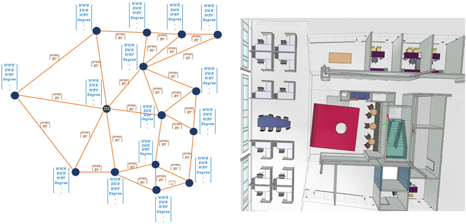
FIGURE 1. Sample building layout and corresponding graph representation.

3.2 Energy Use Intensity (EUI) calculation

This research uses the ground-truth value as the reference value for training the proposed classification model and evaluating its accuracy. To simulate the energy in the case study BIM data, we used RETScreen software, an energy modeling package developed by the Government of Canada. Energy modeling, or energy system modeling, involves the creation of computer models to analyze energy systems and their components. It enables the evaluation and simulation of energy-related scenarios and the assessment of system performance and efficiency. This research uses energy modeling inputs such as building thermal envelope characteristics, ventilation loads, equipment efficiencies, lighting power densities, and plug loads from ASHRAE 62.1 and ASHRAE 90.1 standards ((Goel et al., 2014) for the same climate zone). The Energy Use Intensity (EUI) was determined and calculated for each zone to evaluate more critical and energy-intense zones. Energy Use Intensity (EUI) has been defined as the measurement of a zone’s annual energy consumption relative to the area (kWh/m2). If the EUI for zone A is higher than zone B, it indicates that zone A consumes more energy per square meter annually. This difference in EUI suggests that various parameters contribute to the higher energy consumption in zone A. The main effective parameters which are considered in our research are summarized below:

3.2.1 Exterior wall thermal resistance

Thermal resistance across the wall is the sum of the resistances of the individual layers. Also known as R-Value, the higher the R-Value, the more resistance the energy transfer. Windows Thermal Conductivity. The overall coefficient of heat transfer quantifies the thermal conductivity of a window, representing the amount of heat gained or lost between the indoor and outdoor environments based on the temperature difference. Also known as the U-Factor, the lower value of the U-factor represents the better the window’s thermal performance.

3.2.2 Zone’s location (room location)

Zones with exterior walls and windows or adjacent to an interior zone with different temperature requirements have higher energy consumption due to heat transfer than internal zones with isometric walls. Window-to-Wall Ratio. Zones with more windows in their exterior walls require more heat in winter and cooling in summer to offset the heat transfer. Zones with different space types might have different lighting requirements. For instance, offices require more lighting than storage or restroom space type. Space type or zone functionality is essential in energy consumption for each zone. For example, ASHRAE 62.1 mandates mechanical designers to provide fresh air to different zones based on the occupancy density presented in the standard. For intense, meeting rooms have an occupancy intensity of 50 people/100 m2 compared to 5 people/100 m2 for offices. This means that meeting rooms require more energy than offices to provide fresh air. Also, designers need to provide more cooling in more occupied spaces because of the internal heat gain of 130 W/person. Total energy consumption is calculated based on mentioned parameters, and the EUI value is calculated by dividing the total energy consumption of a building by its corresponding floor area. This ratio provides a standardized energy efficiency measure and allows for comparison between different buildings or spaces.

3.3 NE-GraphSAGE algorithm for room classification

This research aims to address the room classification task related to energy consumption by employing a graph-based learning algorithm that incorporates the spatial relationships (topology) between rooms. The aim is to identify and classify critical zones within the building based on their energy consumption patterns. The room classification task is the type of GNN node classification in BECE analysis. For BECE-based classification, we applied an inductive GNN method based on GraphSAGE. In this research, the choice of an inductive method over a transductive method is motivated by the need to build a generic model capable of predicting new nodes (rooms) based on observed training data. Transductive learning, like GCN, constructs a model specific to the training and testing data it has already encountered, which is unsuitable for our research application. In retrofitting processes, where buildings undergo structural changes and new spaces are added or demolished, it is crucial to have a model that can accommodate new data and spaces. Thus, an inductive approach allows us to design and train a model for such scenarios. GraphSAGE is an inductive learning algorithm leveraging node features (e.g., node profile information, node degrees) to generate node embeddings (Hamilton, Ying, and Leskovec, 2017). The main idea of GraphSAGE is to consider features from the local neighbors of a node. Specifically, the GraphSAGE forward propagation algorithm feeds the neighbor features into an aggregator function (e.g., mean, pooling). Then its output updates the node in the next layer (or depth). Therefore, it considers node features in the process of embedding and training. In BECE-based classification, node features (attributes of rooms) and edge features (relations between rooms) play an essential role in identifying critical spaces with inefficiency areas; thus, designing a GNN algorithm that can process both nodes and edge features is desired. However, the GraphSAGE algorithm is limited to node-level features, which is insufficient for this task. Therefore, this research improves the GraphSAGE algorithm by introducing the Node-Edge GraphSAGE (NE-GraphSAGE) method, which involves node and edge features in the training and classification process.

NE-GraphSAGE aims to learn a representation for every node and corresponding edge based on some combination of its neighboring nodes, parametrized by h for the node and e for the edge. Recall that every node can have its feature vector parameterized by X. Each edge has its feature vector parameterized by Y. Let us assume that all the feature vectors for every node and edge are the same size. One layer of NE-GraphSAGE can be run for k iterations. Parameter k controls the neighborhood depth. If k is 1, only the adjacent nodes are involved in the learning process. If k is 2, the nodes at walk depth two are considered.

${\mathit{h}}_{\mathit{v}}^{\mathit{k}-\mathbf{1}}={\mathit{h}}_{\mathit{v}}^{\mathbf{0}}={\mathit{X}}_{\mathit{v}}(1)$

The following statements represent the definitions of the notations:

$\begin{array}{c}{\mathit{X}}_{\mathit{v}}=Nodefeaturesforanodev\\ {\mathit{Y}}_{\mathit{u}\mathit{v}}=edgefeaturesfornodeuandv\\ {\mathit{h}}_{\mathit{v}}^{\mathit{k}}=embeddingfeaturesnodevinneighbourdepthk\\ {\mathit{e}}_{\mathit{u}\mathit{v}}^{\mathit{k}}=embeddingfeaturesedgeuvinneighbourdepthk\\ {\mathit{N}}_{\mathit{v}}=neighboursetofNodev\\ {\mathit{Z}}_{\mathit{v}}=targetnodeembeddingrepresenation\end{array}(2)$

Remark that having k = 2 means nodes at neighborhood depth two can affect each other through the node in the middle; therefore, there is a node (space) representation h for every node at every k iteration. The value of k is determined experimentally using multiple neighborhoods. We can construct a computation graph for each node that represents the k-hope neighborhood graph of a target node. The computation graph represents the neighbor nodes of each space and the topology information between them.

Figure 1 illustrates an example of a computation graph of target node 3 with a neighborhood depth of two. The NE-GraphSAGE algorithm follows a three-step process, starting with an initialization step. This step sets all the initial node embedding vectors to their respective feature vectors. The algorithm then iterates over the steps, with k representing the iteration number.

3.3.1 Information aggregation

Once the neighborhood has been defined, the next step is establishing an information-sharing procedure among neighboring nodes. To achieve this, a computational graph is created for each node, which enables the calculation of new embedding (feature) values for the target node. In this process, the computational graph considers the features of the target node as well as the features of its neighboring nodes. By incorporating information from the neighboring nodes, the graph can update and refine the embedding of the target node, capturing its surrounding context’s collective knowledge and characteristics.

This information-sharing procedure plays a crucial role in graph-based learning algorithms, such as GraphSAGE or Graph Attention Networks (GAT), as it allows for the propagation of information across the graph and facilitates the generation of more accurate and meaningful embeddings for each node. In this research, we design Aggregation functions or Aggregators that accept the features from neighborhood nodes and edges as input and aggregate the neighbor’s attributes (features) to create a neighborhood embedding for the target node. We first initialize all node and edge embeddings to node features as the node and edge attributes to learn embeddings with aggregators. Then, for each neighborhood depth until K, we create a node and edge embedding with the aggregator function. This aggregation method helps us use the effect of the neighbor spaces on energy consumption in the learning algorithm process (NE-GraphSAGE). Also, employing the edge’s feature in the learning process, the topology information is applied based on the common area and R-Value between two neighbor and target spaces. Different aggregation functions are LSTM (Long Short-Term Memory) aggregator, Pooling aggregator, and Mean aggregator (Kiavarz et al., 2021). We have chosen the Mean aggregator for this research because of its simplicity in implementation. Eq. 3 demonstrates the proposed aggregation function in which ℎk−1 shows the feature values of the neighbor nodes, ek−1 demonstrates the feature values of edges between neighbor nodes and the target node. In the aggregation process, the mean of neighbor nodes and edges features are calculated, then two result vectors are concatenated in-depth k-1. ${\mathit{h}}_{\mathit{N}\left(\mathit{v}\right)}^{\mathit{k}}$ is the aggregated node and edge representation of node v, considering its neighboring nodes and edges in depth k.

${\mathit{h}}_{\mathit{N}\left(\mathit{v}\right)}^{\mathit{k}}\leftarrow \mathit{C}\mathit{o}\mathit{n}\mathit{c}\mathit{a}\mathit{t}\left({\mathit{M}\mathit{e}\mathit{a}\mathit{n}}_{\mathit{N}\left(\mathit{v}\right)}\left({\mathit{h}}_{\mathit{u}}^{\mathit{k}-\mathbf{1}}\right)\right.,{\mathit{M}\mathit{e}\mathit{a}\mathit{n}}_{\mathit{N}\left(\mathit{v}\right)}\left({\mathit{e}}_{\mathit{u}\mathit{v}}^{\mathit{k}-\mathbf{1}}\right)(3)$

3.3.2 Feature updating

After obtaining an aggregated representation for node $v$ based on its neighbors, update the features of node $v$ using a combination of its previous representation $\left({h_{\left(v\right)}}^{k-1}\right)$ , the aggregated representation $\left({h_{N\left(v\right)}}^{k-1}\right)$ includes the edge representation ( $e_{uv}^{k-1}$ ). This research proposed a new updating and aggregation function to consider both node and edge features during learning. Eq. 4 demonstrates the updating function by concatenating the aggregated representation in depth k-1 and target. Node 3 is an example (Figure 2) representing the proposed algorithms with neighbor nodes of ${\mathrm{h}}_6^1,{\mathrm{h}}_4^1,{\mathrm{h}}_2^1,{\mathrm{h}}_1^1$ and the feature between the target node and neighbors ( ${\mathrm{e}}_{63},{\mathrm{e}}_{43}$ ; ${\mathrm{e}}_{23},{\mathrm{e}}_{13}$ ). By aggregating neighbor nodes and edge features, the vector feature of ${\mathrm{h}}_3^1$ is feeding into the update function in layer 2 (k = 2). In the next step, the vector feature of Node 3 in Layer 2 ( $\left.{\mathrm{h}}_3^2\right)$ and aggregated vector feature of node 3 from layer 1 ( $\left.{\mathrm{h}}_3^1\right)$ are concatenated. The non-linearity $\left(\sigma \right)$ is applied to the result as an activation function. This research applies the Sigmoid activation function (Shrikumar, Greenside, and Kundaje, 2017) because its output is between 0 and 1, suitable for our space binary classification output. The algorithm is implemented in Python script with PyTorch, NumPy, DGL, Panda, and sklearn libraries in the Google colab environment. Then, the concatenated vector is passed to the neural network layer as the last step. Figure 3 the pseudocode of the embedding generation of each node in the depth walk k.

FIGURE 2

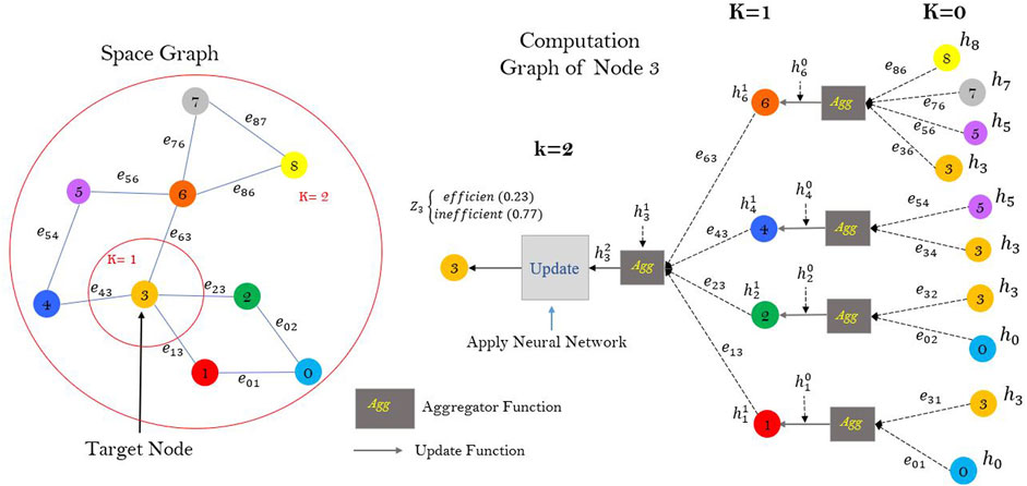
FIGURE 2. Computational Graph of Space 3 with the neighbor depth of 2.

FIGURE 3

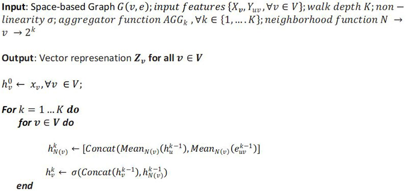
FIGURE 3. The pseudocode of the embedding generation of each node in the depth walk k.

3.3.3 NE-GraphSAGE training

In this step, a multi-layer perceptron neural network (MLP) is designed as a learnable updating process (Figure 4) to update the target node embedding to determine the probability of a critical zone of spaces discussed in the next section. In order to train the neural network and optimize its weights, a differentiable loss function is required. In this study, the Squared Error Loss (SE) function [33] is chosen to calculate the distance between the actual value of the node class (0 or 1) and the predicted values. The Squared Error Loss function measures the square of the difference between the predicted and actual values, penalizing more significant errors more significantly. The neural network aims to minimize the discrepancy between its predictions and the ground truth labels by minimizing this loss function during training. By utilizing the Squared Error Loss function, the neural network can effectively quantify the error in its predictions and adjust its weights to minimize it, leading to improved accuracy and convergence during training. Indeed, compared to other node classification benchmark datasets, the space-based graph in commercial buildings typically does not have many nodes or node features. Commercial building graphs are often smaller in scale and may have fewer nodes and edges than datasets used in other domains. While this may limit the direct applicability of specific graph-based learning algorithms designed for larger graphs, it also presents an opportunity to explore tailored approaches and optimizations specifically suited for the characteristics of space-based graphs in commercial buildings.

FIGURE 4

FIGURE 4. MLP neural network design for space classification.

Unlike other approaches, the room-based graph in this research represents the entire building as a single 3D graph, with each room being represented as a small node and the spatial relationships between rooms as edges. This compact graph representation allows for a holistic analysis of energy consumption patterns within the building, considering the interconnectivity of rooms comprehensively. Therefore, we considered all nodes (spaces) in one patch for the learning process. Instead of involving each node’s feature in the learning step, the embedded vector of the updated feature vector (section 3.2.2) is considered input of the neural network to use the advantage of neighborhood and topology information in the learning process. A two-layer MLP neural network method is designed in which the weighted matric is shared between all computation graphs in the last depth (k). Figure 5 represents a sample computation graph for Node 4 and 5 in which the neural network parameters are shared.

FIGURE 5

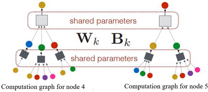
FIGURE 5. Sample computation graphs and shared weighted matrices.

Therefore, the generated computation graph of each building’s space is applied in a batch learning process. Indeed, we employed Batch Gradient Descent (BGD) method for the learning process to update the shared weighted matric (Qi, Wang, and Wang, 2023). We calculate the average gradient across all training examples to update the parameters and use that mean gradient for parameter updates. Therefore, there is just one gradient descent step in one epoch (Figure 6). The distance between the ground truth and the predicted output value is measured by Mean Squared Error (MSE), the function. MSE Eq. 4 is calculated for each iteration (epoch) for all nodes.

FIGURE 6

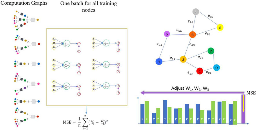
FIGURE 6. Batch gradient descent of the learning process.

At the end of each epoch, the neural network’s weighed matrices are adjusted by the backpropagation process (Linyuan and Zhou, 2011). Then, the learning process is continued iteratively to catch the minimum MSE value.

$MSE=\frac{\mathbf{1}}{\mathit{n}}{\displaystyle \sum _{\mathit{i}=\mathbf{1}}^{\mathit{n}}}{\left({\mathit{Y}}_{\mathit{i}}-\widehat{{\mathit{Y}}_{\mathit{i}}}\right)}^{\mathbf{2}}(4)$

3.3.4 Model interpretation

In addition to accurately applying EN-GraphSAGE for the space classification model in two critical and non-critical zones, we must understand and interpret how and why our models make their predictions. The knowledge gained from the prediction and interpretation models can help planners and engineers to develop more effective strategies and help them manage the demand for energy in different spaces in the buildings. To better understand the classification result, we use a method to investigate the role of each input parameter.

To recognize which parameter(s) has more impact on the result of the space classification as a critical zone or non-critical zone, we need a method to measure and score the contribution of each feature (room properties or neighbor’s relationship) for each node (space). For this purpose, we combined the accurate NE-GraphSAGE method and the explainable ML method SHAP (Shapley Additive exPlanations) to study the critical zones of buildings. In a predictive model, Shapley values Eq. 5 represent the contribution of each input feature to the prediction of each room. Shapley’s values consider the outcomes of all possible combinations of features in a space or edge to determine the importance of each feature. It considers each feature’s contributions in different feature combinations and evaluates their overall impact on the prediction. The set corresponds to each possible combination of space’s features, the neighbor embedder’s features, and the edge’s features contribute to calculating the Sharpley value. In this way, each feature with a higher Sharpley value contributes more to the final result. We interpret the features of all spaces marked as critical Spaces in the classification model to demonstrate more insight into architecture and engineering for accurate decision-making.

${Ø}_i\left(p\right)={\displaystyle \sum _{\left.S\subset N/i\right)}}\frac{\left|S\right|!\left(n-\left|S\right|-1\right)!}{N!}\left(p\left(S\cup i\right)-p\left(S\right)\right)(5)$

The Sharpley values are calculated for features belonging to the spaces marked as critical to explaining the role of each feature in the final output. NE-GraphSAGE can explain the model’s output by calculating the probability of each space (room). If the probability is closed 1, it can be considered a critical space. If it is close to 0, it will be marked as non-critical space. This is called global interpretability. Next, we explain why each space receives the prediction according to its specific predictor (features) values called local interpretability. The Sharply values can show both. For example, Figure 7 represents the force plot of a test node (Room 154) in the first story marked as a critical space.

FIGURE 7

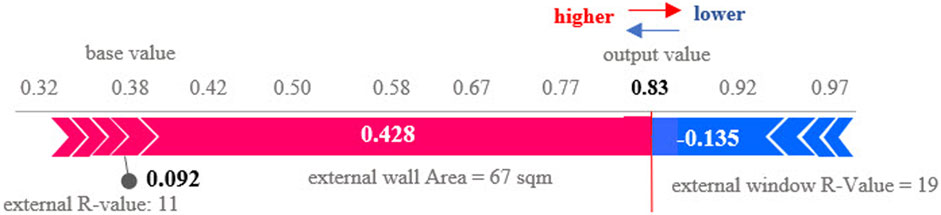
FIGURE 7. SHAP force plot.

The Sharpley value for Room 154 is calculated for all features. The Features with high Shapley values have a more significant impact on model output (0.83 in Figure 6), and features with low Shapley values have less impact on the prediction. This is because the features with the positive Shapley value force the prediction to the output class, and the features with a negative Sharpley value push the output to the other class. In this example, the External Wall Area (EWA) and External Wall R-Value (EWR) have the most positive Sharpley value of 0.428 and 0.092, which impacts the energy consumption of Room 154 and push it into the critical space class. The emergence of this insight provides valuable information for architects and engineers, enabling them to focus on optimizing the wall geometry design and enhancing the insulation materials used in Room 154 to reduce its energy intensity. Additionally, the negative Shapley value associated with the External Window R-Value (EWINR) suggests that the window material insulation is already in good condition and does not contribute significantly to the room’s energy consumption.

4 Experimental results and discussion

We apply the proposed methodology to a three-story IFC model collected from open IFC model datasets. The proposed classification model’s results and the interpretation models to explain the classification results are presented in the following sections.

4.1 NE-GrahSAGE classification model

The BIM data as the case study is downloaded from the Open IFC Model Repository in IFC format. It includes 130 spaces with different activities, including an office room, conference room, lounge, kitchen lobby, and washroom. The Energy Use Intensity (EUI) (Ma and Cheng 2016) is considered an energy consumption index in this research. First, a ground-truth value is calculated for all spaces for three stories using RETScreen software to perform energy modeling for multiple zones in this paper. The Energy Use Intensity (EUI) measures annual energy consumption per square foot. It is obtained by dividing the total energy consumed by the building in a year by its total floor area. Next, the total energy is estimated for each space using RETScreen software by considering space geometry information, material information, heating and cooling energy to keep the comfortable temperature, thermal envelope characteristics, ventilation loads, equipment efficiencies, lighting power densities, and plug loads were taken from ASHRAE 62.1 and ASHRAE 90.1 40. Standards for building climate zone. Then, Z-score 41. Is calculated for EUI values to find an outlier. The spaces with outliers EUI values are considered critical spaces. In the last step, EN-GraphSAGE is employed to classify the nodes on the space-based graph to classify the spaces in critical and non-critical spaces. The best accuracy achieved during the range of epochs from 1000 to 5000 was 91.26%, occurring at epoch 3500. Therefore, we pick up the weight matrices in epoch 3500. To assess the accuracy and correctness of each classifier, we utilized two commonly used metrics: accuracy and F1 score. These metrics provide a quantitative measure of the classification performance. We evaluated the performance of four well-known classification methods: NE-GraphSAGE, GraphSAGE, ANN, and SVM. Accuracy is a reliable criterion for assessing overall correctness, as it represents the fraction of correct predictions over the total number of samples, regardless of their respective classes. It is calculated using Eq. 6, where the numerator represents the number of correct predictions and the denominator represents the total number of samples. The F1 score is another important metric that considers both precision and recall. It provides a balanced measure of the classifier’s performance by considering positive and negative class predictions. However, the specific calculation for the F1 score is not mentioned in the given context. By evaluating the accuracy and F1 score of the four classification methods, we can gain insights into their performance and determine their effectiveness in the context of the problem being addressed. Accuracy may be biased towards predominant classes, so we used the F1 score as an evaluation metric to assess balanced predictions. The F1 score calculates each class’s harmonic mean of precision and recall and then takes the arithmetic mean across all classes Eq. 7.

$\begin{array}{c}Accuracy=\frac{{\sum }_{i}T{P}_i}{N_n}\\ \text{TP}=\text{true\hspace{0.17em}positive},\\ \text{Nn}=\text{number\hspace{0.17em}of\hspace{0.17em}nodes}\end{array}(6)$

The accuracy and F1 are calculated for four graph-based (NE-GraphSAGE, GraphSAGE) and none graph-based (ANN and SVM) methods to compare the result of the proposed method with other classification methods (Table 1).

$F1=\frac{{\displaystyle \sum _{i=1}^n}\frac{2\times T{P}_i}{2\times T{P}_i+F{P}_i+F{N}_i}}{n}(7)$

TABLE 1

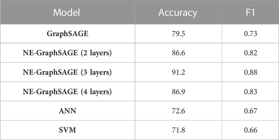
TABLE 1. Classification models accuracy and F1 score.

TP = true positive, FP = false positive, FN = false negative, n = number of classes.

We prove that the proposed classification method (NE-GRAPHSAGE (3 layers) provides significant gains (12% on average) compared to other classification methods, especially non-graph-based methods, which have the highest accuracy and F1 from the experiment results, arriving at 91.2% and 0.88, respectively. On the other hand, NE-GraphSAGE (2 layers) and NE-GraphSAGE (4 layers) have slightly lower accuracy, and F1 with less balanced prediction compared to NE-GraphSAGE (layers3). We also trained GraphSAGE with three layers for a comprehensive comparison. We used the same dataset and fine-tuned GraphSAGE to obtain its best results. The difference between the two algorithms is that NE-GraphSAGE can consider both node and edge features during updating embedding, while GraphSAGE only learns from node features. As a result, NE-GraphSAGE (3 layers) improved the accuracy by 12% and the F1 score by 0.15 compared with GraphSAGE. Also, the result recognized the effect of edge features (topology features) in finding the critical zones. For example, six interior rooms are wrongly marked as non-critical zones by non-graph-based methods, but two graph-based methods classified these rooms correctly as critical spaces. This is because these rooms are in the neighborhood of critical spaces with a low R-value of shared walls on the first and third floors. However, they are classified as non-critical spaces for those models where the topology information is ignored in the learning process.

Consequently, NEGraphSAGE (3 layers) generally has the highest accuracy and most balanced prediction performance. Therefore, NE-GraphSAGE (3 layers) is chosen as the room classification algorithm in this research compared to other algorithms. Hence, in the remainder of the paper, the term NE-GraphSAGE refers to the 3-layer variant of NE-GraphSAGE.

4.2 Interpreting EN-GraphSAGE classification using SHAP values

The SHAP method is employed on the result of test data to assign a Sharpley value for features in each space considered a critical zone. The impact of features on the prediction of critical zone probability for each space is measured by evaluating the deviation from the mean predicted value when different combinations of features are utilized. In addition, this paper uses a forced plot to find feature importance, interpretation, and parameter(s) that cause high energy consumption in these zones. We calculated the Sharply value of features for those spaces classified as critical zones. As the proposed classification model considered the space’s properties and adjacency information, the Sharpley values can be calculated for both feature sets. Therefore, the SHAP method in this research can pinpoint which parameters of the room of its adjacent rooms are most impactful for high energy consumption. For every space, the features are ordered by their Sharpley value. Some of those features negatively affect energy consumption, and these form the basis for the expert recommendation in process design or retrofitting to increase energy efficiency. Figure 8 represents the force plot for Space-153, which shows the Sharpley value normalized between 0 and 1.

FIGURE 8

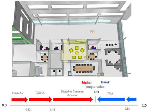
FIGURE 8. SHAP force-plot for Room 153.

Considering all features, the Sharpley value for Room 153 is estimated at 0.71. The neighbor common R-value is the primary parameter pushing this room as a critical class. Although the boarding room has no external wall or window, it has pinned as the critical zone. It is in the neighborhood of critical space-154, and a high energy rate is transferred between these two rooms. Therefore, this room recommends using different window materials (with higher R-value) between them.

5 Conclusion

This paper introduced a new GNN-based classification model (NE-GraphSAGE) to find the critical zone using a 3D building model. This model considers the space’s properties and the adjacent information in training the classification model. The promising result demonstrates a better model accuracy than the non-graph base and regular GraphSAGE models. In order to address the trade-off between model accuracy and interpretability, the NE-GraphSAGE model is combined with the SHAP (SHapley Additive exPlanations) model. SHAP is a method used for model interpretation that provides explanations for individual predictions. By incorporating SHAP with the NE-GraphSAGE model, the researchers aim to achieve high accuracy and interpretability. This allows for a better understanding of the factors influencing the model’s predictions, enhancing the transparency and trustworthiness of the model’s results. Instead of choosing between accuracy and interpretability, the proposed methodology finally proposed a solution that lets us push the envelope regarding model complexity and accuracy while still allowing us to derive intuitive explanations for each space. Also, the proposed interpretation model can explain the impact of individual features in a room and aggregated features in 3D adjacent rooms. The result shows that combining the high-accuracy classification model (NE-GraphSAGE) and the SHAP model can help designers and engineers have accurate insight into their design and decision-making process. However, this methodology has two main limitations that need future work.

The first limitation addresses the adjacent interception. Although we can find the Sharpley value for adjacent features, we cannot find which exactly adjacent room(s) has more impact on the target room because the adjacent feature values result from the aggregation function. The second limitation is that the knowledge expert should explain the recommendation. The proposed methodology can find and explain the reason for classification results but is limited to using the result for the recommendation and prescription. The latter ones are ongoing research, and the outcome of the research will be presented in the near future.

Data availability statement

Publicly available datasets were analyzed in this study. This data can be found here: http://openifcmodel.cs.auckland.ac.nz.

Author contributions

HK: Conceptualization, Data curation, Formal Analysis, Investigation, Methodology, Software, Validation, Visualization, Writing–original draft, Writing–review and editing. MJ: Conceptualization, Investigation, Software, Writing–original draft, Writing–review and editing, Formal Analysis, Funding acquisition, Methodology, Project administration, Resources, Supervision, Validation. PE: Conceptualization, Methodology, Validation, Writing–review and editing.

Funding

The author(s) declare financial support was received for the research, authorship, and of this article. This research was funded by the Natural Sciences and Engineering Research Council of Canada (NSERC DG 485794) and York University.

Acknowledgments

The authors would like to thank Autodesk for providing open-source BIM data for this study. We would also like to thank the three reviewers for their feedback, which has helped improve the quality of the manuscript.

Conflict of interest

Author PE was employed by Program Manager Willdan Energy Solutions.

The remaining authors declare that the research was conducted in the absence of any commercial or financial relationships that could be construed as a potential conflict of interest.

Publisher’s note

All claims expressed in this article are solely those of the authors and do not necessarily represent those of their affiliated organizations, or those of the publisher, the editors and the reviewers. Any product that may be evaluated in this article, or claim that may be made by its manufacturer, is not guaranteed or endorsed by the publisher.

References

Ahmad, A. S., Hassan, M. Y., Abdullah, M. P., Rahman, H. A., Hussin, F., Abdullah, H., et al. (2014). A review on applications of ANN and SVM for building electrical energy consumption forecasting. Renew. Sustain. Energy Rev. 33, 102–109. doi:10.1016/j.rser.2014.01.069

CrossRef Full Text | Google Scholar

Ahmad, T., and Zhang, D. (2020). A critical review of comparative global historical energy consumption and future demand: the story told so far. Energy Rep. 6, 1973–1991. doi:10.1016/j.egyr.2020.07.020

CrossRef Full Text | Google Scholar

Atila, U., Ismail Rakip, K., and Alias Abdul, R. (2013). “A 3D-GIS implementation for realizing 3D network analysis and routing simulation for evacuation purpose,” in Lecture notes in geoinformation and cartography (Berlin, Germany: Springer). doi:10.1007/978-3-642-29793-9-14

CrossRef Full Text | Google Scholar

Celik, S., Roxana, F., and Pinar Menguc, M. (2016). Analysis of perlite and pumice based building insulation materials. J. Build. Eng. 6, 105–111. doi:10.1016/j.jobe.2016.02.015

CrossRef Full Text | Google Scholar

Chalal, M., Benachir, M., White, M., and Shrahily, R. (2016). Energy planning and forecasting approaches for supporting physical improvement strategies in the building sector: A review. Renew. Sustain. Energy Rev. 64, 761–776. doi:10.1016/j.rser.2016.06.040

CrossRef Full Text | Google Scholar

Collins, F. C., Braun, A., Ringsquandl, M., Hall, D. M., and Borrmann, A. (2021). Assessing IFC classes with means of geometric deep learning on different graph encodings. Proc. 2021 Eur. Conf. Comput. Constr. 2, 332–341. doi:10.35490/ec3.2021.168

CrossRef Full Text | Google Scholar

Duval, A., and Malliaros, F. D. (2021). “GraphSVX: shapley value explanations for graph neural networks,” in Lecture notes in computer science (including subseries lecture notes in artificial intelligence and lecture notes in bioinformatics) 12976 LNAI (New York, NY, USA: Springer International Publishing), 302–318. doi:10.1007/978-3-030-86520-7_19

CrossRef Full Text | Google Scholar

Fumo, N. (2014). A review on the basics of building energy estimation. Renew. Sustain. Energy Rev. 31, 53–60. doi:10.1016/j.rser.2013.11.040

CrossRef Full Text | Google Scholar

Goel, R., Xie, A., Wang, H., and Zhang, M. (2014). Enhancements to ASHRAE standard 90.1 prototype building models. Richland, WA, USA: Pacific Northwest National Lab.

Google Scholar

Hamilton, W. L., Ying, R., and Leskovec, J. (2017). Inductive representation learning on large graphs. Adv. Neural Inf. Process. Syst. 30. doi:10.48550/arXiv.1706.02216

CrossRef Full Text | Google Scholar

Ismail, A., Strug, B., and Ślusarczyk, G. (2018). “Building knowledge extraction from BIM/IFC data for analysis in graph databases,” in Proceedings of the Artificial Intelligence and Soft Computing: 17th International Conference, ICAISC 2018, Zakopane, Poland, June 2018, 652–664. doi:10.1007/978-3-319-91262-2_57

CrossRef Full Text | Google Scholar

Jin, C., Xu, M., Lan, L., and Zhou, X. (2018). “Exploring BIM data by graph-based unsupervised learning,” in Proceedings of the 7th International Conference on Pattern Recognition Applications and Methods, Funchal, Portugal, January 2018. doi:10.5220/0006715305820589

CrossRef Full Text | Google Scholar

Khalili, A., and H Chua, D. K. (2015). IFC-based graph data model for topological queries on building elements. J. Comput. Civ. Eng. 29 (3), 04014046. doi:10.1061/(ASCE)CP.1943-5487.0000331

CrossRef Full Text | Google Scholar

Kiavarz, H., Jadidi, M., Rajabifard, A., and Sohn, G. (2023). An automated space-based graph generation framework for building energy consumption estimation. Buildings 13 (2), 350. doi:10.3390/buildings13020350

CrossRef Full Text | Google Scholar

Kiavarz, H., Jadidi, M., Rajabifard, A., and Sohn, G. (2021). “ROOM-BASED energy demand classification of BIM data using graph supervised learning,” in Proceedings of the International Archives of the Photogrammetry, Remote Sensing and Spatial Information Sciences XLVI-4/W4, Würzburg, Germany, October 2021, 97–100. doi:10.5194/isprs-archives-XLVI-4-W4-2021-97-2021

CrossRef Full Text | Google Scholar

Li, Q., Meng, Q., Cai, J., Yoshino, H., and Mochida, A. (2009). Applying support vector machine to predict hourly cooling load in the building. Appl. Energy 86 (10), 2249–2256. doi:10.1016/j.apenergy.2008.11.035

CrossRef Full Text | Google Scholar

Li, X., Ding, L., Jinhu, L., Xu, G., and Li, J. (2010). “A novel hybrid approach of KPCA and SVM for building cooling load prediction,” in Proceedings of the 3rd International Conference on Knowledge Discovery and Data Mining, WKDD, Newport Beach, CA, USA, August 2010. doi:10.1109/WKDD.2010.137

CrossRef Full Text | Google Scholar

Linyuan, L. L., and Zhou., T. (2011). Link prediction in complex networks: A survey. Phys. A Stat. Mech. Its Appl. 390, 1150–1170. doi:10.1016/j.physa.2010.11.027

CrossRef Full Text | Google Scholar

Naser, M. Z. (2021). An engineer’s guide to EXplainable artificial intelligence and interpretable machine learning: navigating causality, forced goodness, and the false perception of inference. Automation Constr. 129, 103821. doi:10.1016/j.autcon.2021.103821

CrossRef Full Text | Google Scholar

Nouvel, R., Zirak, M., Dagtageeri, H., Coors, V., and Eicker, U. (2014). “Urban energy analysis based on 3d city model for national scale applications,” in Proceedings of the 5th German-Austrian IBPSA Conference, Weimar, Germany, September 2022.

Google Scholar

Pauwels, P., and Walter, T. (2016). EXPRESS to OWL for construction industry: towards a recommendable and useable IfcOWL ontology. Automation Constr. 63, 100–133. doi:10.1016/j.autcon.2015.12.003

CrossRef Full Text | Google Scholar

Pérez-Lombard, L., Ortiz, J., and Pout, C. (2008). A review on buildings energy consumption information. Energy Build. 40 (3), 394–398. doi:10.1016/j.enbuild.2007.03.007

CrossRef Full Text | Google Scholar

Qi, H., Wang, F., and Wang, H. (2023). Statistical analysis of fixed mini-batch gradient descent estimator. J. Comput. Graph. Statistics, 1–13. doi:10.1080/10618600.2023.2204130

CrossRef Full Text | Google Scholar

Saad, M., Zhang, Y., Tian, J., and Jia, J. (2023). A graph database for life cycle inventory using Neo4j. J. Clean. Prod. 393, 136344. doi:10.1016/j.jclepro.2023.136344

CrossRef Full Text | Google Scholar

Saini, L., Raj, B. P., Agarwal, N., Kumar, A., and Kumar, A. (2022). Net zero energy consumption building in India: an overview and initiative toward sustainable future. Int. J. Green Energy 19 (5), 544–561. doi:10.1080/15435075.2021.1948417

CrossRef Full Text | Google Scholar

Shi, W., and Rajkumar, R. (2020). “Point-GNN: graph neural network for 3D object detection in a point cloud,” in Proceedings of the 2020 IEEE/CVF Conference on Computer Vision and Pattern Recognition (CVPR), Seattle, WA, USA, June 2020, 1708–1716. doi:10.1109/CVPR42600.2020.00178

CrossRef Full Text | Google Scholar

Shrikumar, A., Greenside, P., and Kundaje, A. (2017). “Learning important features through propagating activation differences,” in Proceedings of the 34th International Conference on Machine Learning, ICML, Sydney, Australia, August 2017.

Google Scholar

Simeone, D., and Cursi, S. (2017). “A platform for enriching BIM representation through semantic web technologies,” in Lean and computing in construction congress (Edinburgh, Scotland: Heriot-Watt University), 1, 423–430. doi:10.24928/JC3-2017/0323

CrossRef Full Text | Google Scholar

Teske, S., Pregger, T., Simon, S., and Tobias, N. (2018). High renewable energy penetration scenarios and their implications for urban energy and transport systems. Curr. Opin. Environ. Sustain. 30, 89–102. doi:10.1016/j.cosust.2018.04.007

CrossRef Full Text | Google Scholar

Veličković, P., Cucurull, G., Casanova, A., Romero, A., Pietro, L., and Bengio, Y. (2017). Graph attention networks. Available at: http://arxiv.org/abs/1710.10903.

Google Scholar

Wang, J., Wiens, J., and Scott, L. (2020). Shapley flow: A graph-based approach to interpreting model predictions. Available at: http://arxiv.org/abs/2010.14592.

Google Scholar

Wang, Z., and Srinivasan, R. S. (2017). A review of artificial intelligence based building energy use prediction: contrasting the capabilities of single and ensemble prediction models. Renew. Sustain. Energy Rev. 75, 796–808. doi:10.1016/j.rser.2016.10.079

CrossRef Full Text | Google Scholar

Wang, Z., Sacks, R., and Yeung, T. (2021). Exploring graph neural networks for semantic enrichment: room type classification. Automation Constr. 134, 104039. doi:10.1016/j.autcon.2021.104039

CrossRef Full Text | Google Scholar

Xu, M. (2021). Understanding graph embedding methods and their applications. SIAM Rev. 63 (4), 825–853. doi:10.1137/20M1386062

CrossRef Full Text | Google Scholar