Experimental benchmark control problem for multi-axial real-time hybrid simulation

1 Introduction

The need to validate new technologies and increasingly study more complex structural engineering designs demands new experimental techniques for realistic large-scale structural experimentation. Real-time hybrid simulation (RTHS) is a disruptive technology that has evolved over the past 20 years to enable the examination of dynamic systems, especially when traditional testing approaches cannot be employed. However, despite the fact that RTHS has matured considerably in recent years, there are still important gaps in knowledge that prevent its standardization and broad utilization in research and industry (Tian et al., 2020; Palacio-Betancur and Gutierrez Soto, 2022; Home, 2023; Najafi et al., 2023).

A research agenda for this class of techniques (Hybrid Si mulation for Multi-hazard Engineering A Research Agenda Year 1, 2018; Hybrid Simulation for Multi-hazard Engineering A Research Agenda Year 2, 2019) has been established to capture the challenges and priorities for the research community that are necessary to advance the theory and science in this field. Among these challenges, advancing RTHS methods to readily handle multi-dimensional problems have great potential for enabling more advanced testing and synergistically using existing laboratory facilities that have the capacity for such experimentation (Elnashai et al., 2006; Abbiati et al., 2017; Cao et al., 2020; MAST Laboratory, 2023). To develop multi-dimensional RTHS techniques, it is especially important to investigate new control methodologies, enforcement of complex boundary conditions, and real-time computational platforms capable of performing large amounts of computation as the problem escalates. Overcoming these challenges will facilitate a more realistic examination of the dynamic behavior of structural systems.

Multi-dimensional RTHS pursues the preservation of the multiple-degree-of-freedom (MDOF) response of the numerical and experimental substructures. This approach requires that more than one hydraulic actuator exerts the required motion to the experimental substructure demanding the implementation of multiple-input multiple-output (MIMO) control strategies. For instance, the use of multiple actuators in RTHS has enabled the experimental testing of multi-story building specimens where each actuator is connected directly at each story level (Phillips et al., 2013; Friedman et al., 2014; Gao et al., 2014). Considering the influence of the stiffness of the experimental substructure on the coupling of dynamics in the hydraulic actuators, the RTHS performance might be decreased leading to loss of accuracy and instabilities when this coupling is strong (Wallace et al., 2005; Jung et al., 2007; Chae et al., 2014). When the complexity of the problem demands to increase the number of degrees of freedom (DOF) to be enforced at a given interface boundary condition, it is necessary to include supplementary physical components or multi-axial loading systems such as high stiff links or couplers creating a challenging class of RTHS called multi-axial RTHS (maRTHS) (Blakeborough et al., 2001; Darby et al., 2002; Bonnet et al., 2007; Phillips et al., 2013; Friedman et al., 2014; Gao et al., 2014; Najafi and Spencer, 2021; Botelho and Christenson, 2015; Dong et al., 2015; Na et al., 2016; Fermandois and Spencer, 2017; Najafi et al., 2020; Botelho et al., 2022; Liqiao et al., 2022; Park et al., 2022). This type of multi-axial hydraulic actuator assemblages requires nonlinear coordinate transformations that adds additional complexity to nonlinearities, uncertainties, internal coupling, etc. (Nakata et al., 2007; Nakata et al., 2010), which need further investigation. Therefore, there is a clear need to study the complex aspects of maRTHS and, equally important, to disseminate this knowledge and engage the RTHS community by creating opportunities to contribute to understanding the different characteristics of maRTHS.

Benchmark problems have been an effective instrument over the past 30 years to explore how to address specific technical challenges such as structural control and structural health monitoring methods, while also advancing understanding and promoting capacity building (Spencer et al., 1998a; Spencer et al., 1998b; Ohtori et al., 2004; Yang et al., 2004; Nagarajaiah and Narasimhan, 2006; Narasimhan et al., 2006; Nagarajaiah et al., 2008; Narasimhan et al., 2008; Agrawal et al., 2009; Nagarajaiah et al., 2009; Tan et al., 2009; Sun et al., 2016).

In the RTHS community much of the past work has focused on one-dimensional motion using a single hydraulic actuator. A benchmark problem that was developed for the RTHS community has been useful to systematically identify the limitations and capabilities of methodologies and procedures involved in conducting RTHS. A benchmark problem should include: representative models of the components involved, realistic constraints on the hardware and software employed, and meaningful and objective metrics for assessing the success of a particular design strategy. Generally, this is coupled with a code package that provides the participant with a framework for testing out proposed approaches through virtual RTHS (vRTHS). Overall, the impact of these efforts indicates that these benchmark problems have helped to develop and validate different single-input single-output (SISO) control and to define the scientific and technical needs for developing the next-generation of RTHS methods (Najafi et al., 2023).

The earlier RTHS benchmark control problem based on a single actuator and interface point is described in (Silva et al., 2020). The problem statement is focused on developing tracking controllers where the axial displacement of the hydraulic actuator coincides with the lateral displacement of a steel frame specimen. Several partitioning configurations and plant uncertainties are considered to encourage participants to establish robust control designs while also advancing the understanding of the relationship between controller performance and test objectives (Maghareh et al., 2014; Maghareh et al., 2017). To date, at least fifteen participants have taken part in addressing that benchmark problem, and many lessons were extracted. For instance, it has been demonstrated that robust methodologies based on linear-quadratic-gaussian controllers and model-based compensation techniques handle uncertainties effectively while maintaining low (∼3%) tracking errors (Fermandois, 2019; Zhou et al., 2019). Participants have also implemented and assessed adaptive control techniques and state estimators to enhance the tracking control performance reducing errors due to modeling uncertainties, time delays, and time lags (Xu et al., 2019; Xu et al., 2019; Najafi and Spencer, 2019; Ning et al., 2019; Ouyang et al., 2019; Palacio-Betancur and Gutierrez Soto, 2019; Tao and Mercan, 2019; Wang et al., 2019) to ∼1%–6%. Explicit nonlinear approaches such as sliding mode control have also been applied to manage the uncertainties successfully resulting in tracking errors of ∼0.6%–2% (Xu et al., 2019; Li et al., 2021). Other approaches have been proposed such as impedance matching (Verma and Sivaselvan, 2019) and reinforcement learning (Li et al., 2022), which exhibit promising results for increasing RTHS performance. Furthermore, innovative methodologies for conducting RTHS have also been reported. (Gao and You, 2019). developed a methodology for quantifying predictive measures to analyze the stability limits of an RTHS partition at the early stage of its implementation, which is useful to assess the feasibility of such implementation. The broad engagement in this benchmark problem reveals the importance of having a ready-to-use and standardized virtual RTHS environment. Participants can concentrate their efforts on developing controller methodologies, examining performance, and comparing tracking and RTHS performance. As a result, it accelerates the evolution of the next-generation of controllers for RTHS and confronts specific challenges to overcome such as nonlinear and multidimensional RTHS.

Now, for the same relatively stiff steel frame specimen, a new maRTHS benchmark problem focused on a frame subjected to seismic loading at the base is proposed. This problem aims to elevate the discussion by considering both translation and rotation for tracking control. This seemingly simple, yet fundamental change in the control objectives, considerably transforms the problem and escalates its complexity. This more challenging maRTHS benchmark problem statement presents the experimental setup, problem objectives, evaluation metrics, and realistic control constraints. Experimental data is provided that can be used for system identification, finite element models, and identified state-space models. A code package is provided that can be used to virtually explore the control of a maRTHS experiment conducted in the Intelligent Infrastructure Systems Laboratory (IISL) at Purdue University. To demonstrate the use of this suite of resources, an integral example of a maRTHS design based on a linear quadratic Gaussian (LQG) controller is included as part of the computational code package. The goals of developing this benchmark problem are to: 1) develop, extend, assess, and validate existing control or new MIMO control strategies; 2) provide a computational tool for comparing and contrasting methods for conducting maRTHS; 3) encourage a transition from typical single-actuator RTHS scenarios to maRTHS experiments; and 4) provide a challenging problem for new researchers to gain experience with maRTHS.

Participants are invited to design realizable MIMO controllers using the framework supplied in the code package and described in this paper. Participants are encouraged to address a variety of aspects of maRTHS, including, but not limited to, the effectiveness and influence of limited enforcement of boundary conditions, internal coupling in the plant, tradeoffs between performance and robustness, and scalability of proposed techniques. We anticipate that the availability of this benchmark problem will encourage and inspire a new generation of RTHS techniques and tests in the future.

2 Reference model

This section presents the structural system and its mathematical description denoted as the reference model for evaluating the performance of this RTHS control problem.

2.1 Reference structure description

The reference structure used in this study is shown in Figure 1. It consists of a steel moment-resisting frame with 3 bays and 3 stories. The beams and columns are made from A36 and A992Fy50 steel, respectively. The beams are built-up sections while the columns are hot-rolled commercially available sections. A scaled El Centro historic record is used as the input ground motion to the system to generate the different responses. A scaling factor of 0.40 is selected to ensure that the lateral displacement of the frame is limited to maintain linear elastic behavior of all structural components.

FIGURE 1

FIGURE 1. Reference structure.

2.2 Description of the finite element model

To evaluate the performance of the RTHS algorithms, this benchmark uses a finite element (FE) model to capture the behavior and response of the reference structure. Figure 2 presents the schematic definition of the geometry and connectivity of the reference system. Each node has three DOFs: two translational DOF along the global x and y-axes; and one rotational DOF, θ around the z-axis, perpendicular to the xy-plane. The numbers in circles near the joints represent the node numeration and the numbers in rectangles close to the middle of beams and columns denote the element numeration. In Figure 2, each set of DOFs for any i-th node is represented by the triplet $\left[x_i{y}_i{\theta }_i\right]$.

FIGURE 2

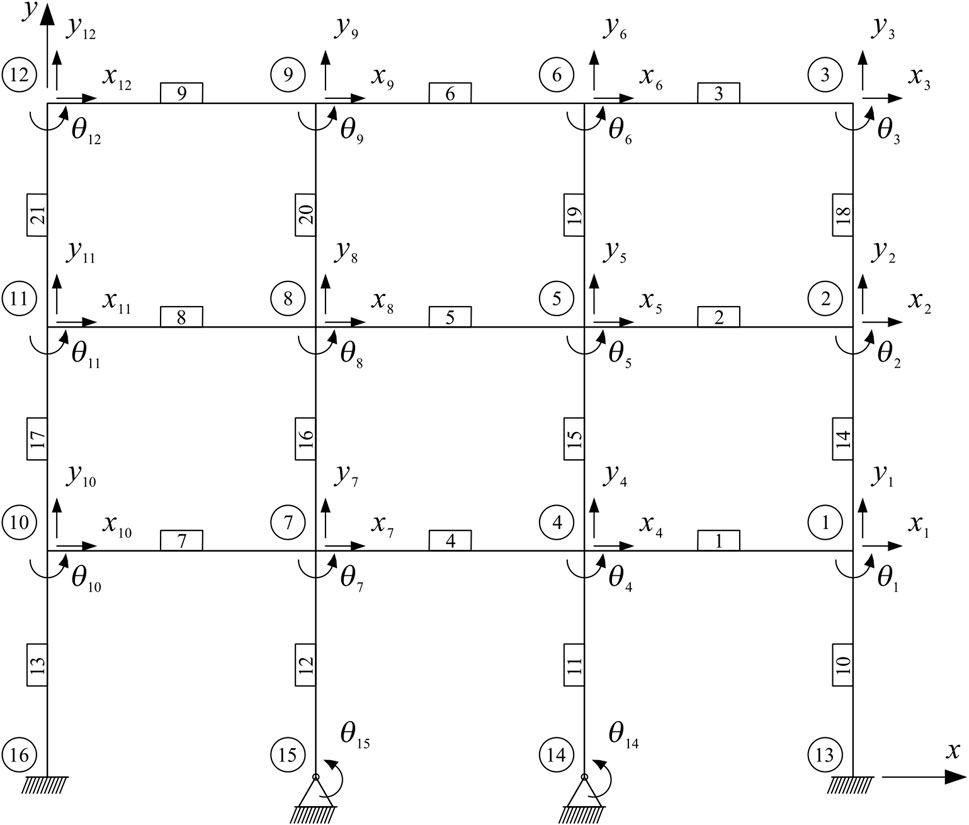
FIGURE 2. FE model description.

The equation of motion for this reference system is given by:

$\mathbf{M}\ddot{\mathbf{\psi }}+\mathbf{C}\dot{\mathbf{\psi }}+\mathbf{K}\mathbf{\psi }=-\mathbf{M}\mathbf{\Gamma }\cdot {\ddot{x}}_{g,}(1)$

where M, C, and K are the mass, damping and stiffness matrices of the reference structure. $\mathbf{\Gamma }$ is an influence vector that describes the inertial effects of the excitation on the masses on the system. In our case this is a column vector that contains a value of one for each mass that develops an inertial effect due to ground acceleration. The one-dimensional variable ${\ddot{x}}_g$ is the ground absolute acceleration and the vectors $\ddot{\mathbf{\psi }}$, $\dot{\mathbf{\psi }}$, and $\mathbf{\psi }$ represent the absolute acceleration, relative velocity and relative displacement with respect to the ground for each degree of freedom considered in our analysis, respectively. Therefore, the number of DOFs in this FE model is 38 and they will be arranged in the displacement vector $\mathbf{\psi }$ according to Eq. (2). Any i-th element of the vector $\mathbf{\psi }$ will be represented by ${\mathit{\psi }}_i$, where $i=1...38$, see Figure 3.

$\mathbf{\psi }={\left[\begin{array}{ccc}{x}_1\dots x_{12}& y_1\dots y_{12}& \begin{array}{cc}\begin{array}{cc}{\theta }_1\dots {\theta }_{12}& {\theta }_{14}\end{array}& {\theta }_{15}\end{array}\end{array}\right]}^T.(2)$

FIGURE 3

FIGURE 3. Definition of the DOF vector in Eq. 2.

For instance, the DOFs of nodes 4 and 7 are represented by the vectors ${\mathbf{\psi }}_4\left[\mathrm{4,16,28}\right]={\left[x_4{y}_4{\theta }_4\right]}^T$ and ${\mathbf{\psi }}_7\left[\mathrm{7,19,31}\right]={\left[x_7{y}_7{\theta }_7\right]}^T$, where the elements in brackets specify particular elements in an array and the subscript designates specific attributes of the array. In these examples, they refer to specific DOFs (element in brackets) of the vector $\mathbf{\psi }$ and their corresponding nodes (subscripts). The first 5 natural frequencies are 2.29 Hz, 12.74 Hz, 26.28 Hz, 26.53 Hz, and 29.91 Hz, with mass participation factors of up to 95%. The damping matrix is calculated here using the Rayleigh damping method with a damping ratio of 5% anchored to first and third modes. The damping matrix is assumed to be proportional to the sum of the mass and stiffness matrices of the reference system:

$\mathbf{C}={\alpha }_1\mathbf{M}+{\alpha }_2\mathbf{K},(3)$

where ${\alpha }_1$ and ${\alpha }_2$ are constants used to generate the desired modal damping ratios for two chosen modes.

3 Benchmark problem definition

This section establishes the structure of the benchmark problem, defines its components, and provides insight to understand the objectives of this MIMO control benchmark problem for maRTHS.

3.1 Reference structure partitioning

To conduct the RTHS, the reference model described in Section 2 must be partitioned into two subdomains: numerical and experimental. The partition chosen is shown in Figure 4. The portion in black (outermost structural elements) represents the numerical substructure, and the portion in red (central frame, simply supported) indicates the physical substructure, which is a steel moment resisting frame available in the IISL and it is assumed to be the less understood part of the entire structure.

FIGURE 4

FIGURE 4. Partitioning: Numerical substructure (black), Experimental substructure (red).

In a partitioned system, these two substructures are separate, but connected to each other and synchronized through a feedback loop so that they share information at common interface nodes at every time step during execution. Figure 5 illustrates the main degrees of freedom of the interface nodes and the signals that transfer information between the numerical and physical substructures. Ideally, during every time interval, the numerical substructure is excited first, then the response of the interface nodes ${\mathbf{\psi }}_{\text{ns}4}\left[\mathrm{4,16,28}\right]={\left[x_{\text{ns}4}{y}_{\text{ns}4}{\theta }_{\text{ns}4}\right]}^T$ and ${\mathbf{\psi }}_{\text{ns}7}\left[\mathrm{7,19,31}\right]={\left[x_{\text{ns}7}{y}_{\text{ns}7}{\theta }_{\text{ns}7}\right]}^T$, and their derivatives (velocity and acceleration) are imposed to the experimental substructure. Afterwards, the generated physical restoring forces, ${\mathbf{f}}_{\text{es}4}={\left[F_{\text{es}4x}{F}_{\text{es}4y}{M}_{\text{es}4}\right]}^T$ and ${\mathbf{f}}_{\text{es}7}={\left[F_{\text{es}7x}{F}_{\text{es}7y}{M}_{\text{es}7}\right]}^T$, are measured and fed back to the numerical substructure. This configuration is usually denoted as ideal RTHS since no additional components such as hydraulic actuators or measured signals contaminated with high frequency noise are considered. Therefore, pure numerical models for the numerical and experimental substructures are used. Herein, the subscript ‘ns’ will be used for variables associated with the numerical substructure, and ‘es’ will be reserved for the experimental substructure variables. This partitioned analysis provides the realization of the most basic hybrid simulation which is helpful when designing and RTHS experiment. It allows one to study the stability of the partitioning chosen, assess the required forces to enforce the boundary conditions in the physical substructure (hence, to evaluate the actuator capacity to be used), define the signals from the physical domain and their structure necessary to close the loop with the specific type of numerical model, etc. For instance, this analysis facilitates the identification of the interface conditions to be enforced in both substructures regardless of whether an ideal RTHS is being executed or a physically actuated RTHS is being conducted. In this benchmark, these key interface conditions are represented by the vectors ${\mathbf{\psi }}_{\text{ns}4}={\left[x_{\text{ns}4}{y}_{\text{ns}4}{\theta }_{\text{ns}4}\right]}^T$, ${\mathbf{\psi }}_{\text{ns}7}={\left[x_{\text{ns}7}{y}_{\text{ns}7}{\theta }_{\text{ns}7}\right]}^T$, ${\mathbf{\psi }}_{\text{es}4}={\left[x_{\text{es}4}{y}_{\text{es}4}{\theta }_{\text{es}4}\right]}^T$, and ${\mathbf{\psi }}_{\text{es}7}={\left[x_{\text{es}7}{y}_{\text{es}7}{\theta }_{\text{es}7}\right]}^T$ in Figure 5.

FIGURE 5

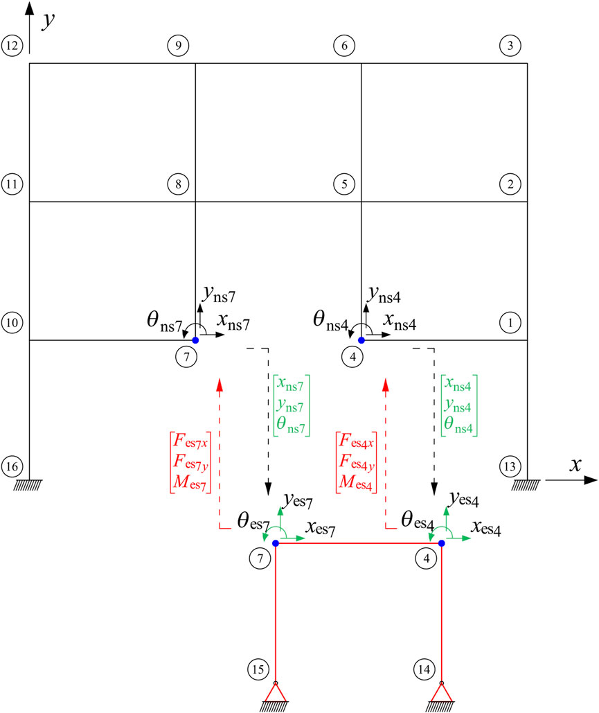
FIGURE 5. Partitioned system in closed loop.

In an actual RTHS implementation, the experimental substructure is physically built and connected to the numerical substructure through a transfer system to ensure dynamic continuity and synchronized motion at common interface nodes during the experiment execution in real time. The inclusion of the transfer system in the experimental domain changes the dynamics of the experimental substructure, and a control approach must be included to compensate for these added dynamics and other effects. This benchmark includes and simulates these components and other relevant effects with identified models based on experimental data. This realistic computational implementation or virtual simulation is called vRTHS, which is the closest realization of an actual RTHS.

3.2 Substructured equation of motion

For RTHS execution, the reference model described in Section 2.1 must be partitioned into numerical and experimental substructures as described in Section 3.1. Assuming linear elastic behavior of the frame, the partitioned mass, damping and stiffness matrices can be written as the sum of numerical and experimental components:

$\left({\mathbf{M}}_{\text{ns}}+{\mathbf{M}}_{\text{es}}\right)\ddot{\mathbf{\psi }}+\left({\mathbf{C}}_{\text{ns}}+{\mathbf{C}}_{\text{es}}\right)\dot{\mathbf{\psi }}+\left({\mathbf{K}}_{\text{ns}}+{\mathbf{K}}_{\text{es}}\right)\mathbf{\psi }=-\mathbf{M}\mathbf{\Gamma }\cdot {\ddot{x}}_g(4)$

where

$\begin{array}{c}\mathbf{M}={\mathbf{M}}_{\text{ns}}+{\mathbf{M}}_{\text{es}}\\ \mathbf{C}={\mathbf{C}}_{\text{ns}}+{\mathbf{C}}_{\text{es}}\\ \mathbf{K}={\mathbf{K}}_{\text{ns}}+{\mathbf{K}}_{\text{es}}\end{array}.(5)$

Herein, the subscript ‘ns’ will be used for variables associated with the numerical substructure, and ‘es’ will be reserved for the experimental substructure variables. The ideal hybrid system with its active DOFs is shown in Figure 6. From this theoretical representation, a numerical substructure model for RTHS is obtained by defining an experimental substructure considering the DOFs ${\psi }_{\text{es}}\left[i\right]$ for i = 4, 7, 16, 19, 28, 31, 37, 38, that are shown in Figure 6. The corresponding matrices ${\mathbf{M}}_{\text{es}}$, ${\mathbf{C}}_{\text{es}}$, and ${\mathbf{K}}_{\text{es}}$ are identified from static loading and free vibration tests, and the numerical substructure matrices are obtained by subtracting the identified experimental substructure matrices from the reference model, which was defined in Section 2. Then, from Eq. (4), the terms associated with the experimental substructure can be arranged into the right-hand side of equation of motion, yielding Eq. (6).

${\mathbf{M}}_{\text{ns}}\ddot{\mathbf{\psi }}+{\mathbf{C}}_{\text{ns}}\dot{\mathbf{\psi }}+{\mathbf{K}}_{\text{ns}}\mathbf{\psi }=-\mathbf{M}\mathbf{\Gamma }\cdot {\ddot{x}}_g-\left({\mathbf{M}}_{\text{es}}\ddot{\mathbf{\psi }}+{\mathbf{C}}_{\text{es}}\dot{\mathbf{\psi }}+{\mathbf{K}}_{\text{es}}\mathbf{\psi }\right)(6)$

${\mathbf{f}}_{\text{es}}={\mathbf{M}}_{\text{es}}\ddot{\mathbf{\psi }}+{\mathbf{C}}_{\text{es}}\dot{\mathbf{\psi }}+{\mathbf{K}}_{\text{es}}\mathbf{\psi }.(7)$

FIGURE 6

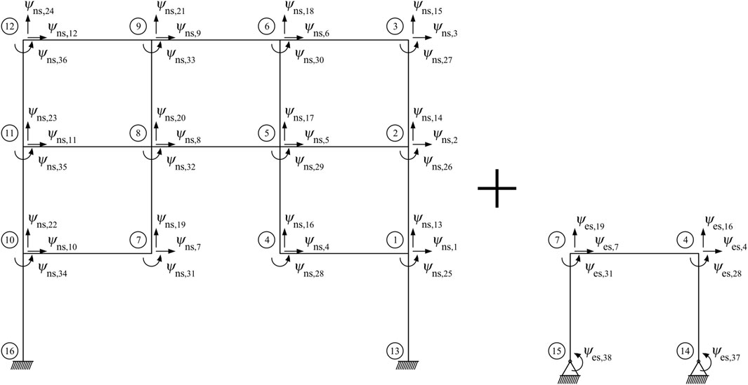
FIGURE 6. Conceptual representation of the reference structure partition.

Here ${\mathbf{f}}_{\text{es}}$ is the feedback force vector produced by the experimental substructure during the dynamic testing. In an ideal RTHS simulation, the feedback force may be obtained directly from Eq. (7). However, in physically actuated RTHS, it must be measured or estimated using measured data from the experimental domain. Finally, dividing the equation of motion by ${\mathbf{M}}_{\text{ns}}$, a mass-normalized form is obtained, see Eq. (8):

$\ddot{\mathbf{\psi }}+{\mathbf{M}}_{\text{ns}}^{-1}{\mathbf{C}}_{\text{ns}}\dot{\mathbf{\psi }}+{\mathbf{M}}_{\text{ns}}^{-1}{\mathbf{K}}_{\text{ns}}\mathbf{\psi }=-{\mathbf{M}}_{\text{ns}}^{-1}\mathbf{M}\mathbf{\Gamma }\cdot {\ddot{x}}_g-{\mathbf{M}}_{\text{ns}}^{-1}{\mathbf{f}}_{\text{es}},(8)$

which, in this benchmark, is numerically integrated using the unconditionally stable constant-average-acceleration Newmark’s method with parameters $\alpha =0.25$ and $\delta =0.5$ (Bathe and Bathe, 2014). The time step is 0.976 ms since the goal is to run this RTHS Benchmark in real time with a sampling frequency of 1,024 Hz.

3.3 Physical substructure geometry and material specifications

The physical specimen in the laboratory will be connected to the numerical substructure of the RTHS experiment. This frame was utilized in previous research (Gao, 2012; Gao et al., 2013) and as part of a past benchmark problem (Silva et al., 2020). Thus, the feasibility of the plant has already been demonstrated. Figure 7 shows the frame and its geometry, which is composed of a horizontal beam and two vertical columns made of structural steel A572 Grade 50. The boundary conditions at the base correspond to pinned connections and the column-beam joints are assumed rigid, transmitting axial, shear, and moment forces. The beam element is fabricated with a 50 mm × 6 mm plate (web) and two 38 mm × 6 mm plates (flanges), forming a custom-made I beam, and the columns are commercially available hot-rolled S3 x 5.7 sections.

FIGURE 7

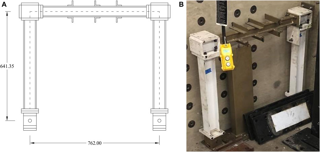
FIGURE 7. Steel frame comprising the physical substructure: (A) Drawing (Units: mm), (B) Photograph.

3.4 Transfer system

In RTHS, additional hardware is needed to drive the experimental frame synchronously with the numerical substructure. The interface conditions discussed in Section 3.1 are enforced by the transfer system which in this case consists of two hydraulic actuators. Hereafter, the vertical DOFs along the global coordinate y will not be considered for convenience, and due to the negligible axial deformations in columns, vertical displacements in the nodes are small in comparison with the horizontal displacements. For instance, Figure 8A shows that for node 4 of the frame, the two associated DOFs of the numerical substructure ${\mathbf{\psi }}_{\text{ns}4}\left[\mathrm{4,28}\right]={\left[x_{\text{ns}4}{\theta }_{\text{ns}4}\right]}^T$ are imposed to node 4 of the experimental substructure (i.e., ${\mathbf{\psi }}_{\text{es}4}\left[\mathrm{4,28}\right]={\left[x_{\text{es}4}{\theta }_{\text{es}4}\right]}^T$). To represent this MDOF response in a more realistic fashion, these two interface boundary conditions are imposed by incorporating a multi-axial testing technique, which requires the use of multiple hydraulic actuators since each actuator provides translational motion only if used independently. Figure 8B illustrates that a minimum of two hydraulic actuators provide equivalent translational and rotational motion to node 4.

FIGURE 8

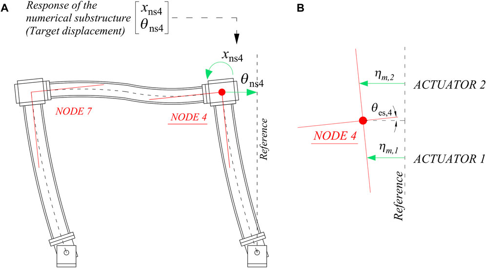
FIGURE 8. Equivalent multi-actuator action to provide both translational and rotational motion. (A) Interface boundary conditions at node 1: rotation and linear displacement, (B) Equivalent MDOF motion performed by two hydraulic actuators.

However, to use these two hydraulic actuators, a supplementary component between the frame and the actuator is designed and fabricated. This element attached to the physical frame is referred to herein as the coupler. The coupling of the linear stroke of both actuators through the coupler results in the translational and rotational motion of the coupler and subsequently the physical frame, as depicted in Figure 9.

FIGURE 9

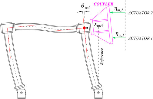
FIGURE 9. Coupler attached at the interface joint enables the use of two hydraulic actuators.

The immediate effect of this setup is the complex internal coupling between the physical frame, coupler, and actuators. To understand these interactions, it is necessary to study each component individually.

3.4.1 Servo-hydraulic actuators

Two fatigue-rated, double-ended, linear servo-hydraulic actuators (ShoreWestern, 910D series), with a nominal force capacity of 9.34 kN (2.2 kip) and a stroke of ±63 mm, are used (see Figure 10). Each actuator has a built-in LVDT (linear variable differential transformer) transducer that collects measurements of linear displacements, and two load cells (Interface, 1,000 series) with a nominal force capacity of 11.2 kN providing instantaneous force measurements. These hydraulic actuators operate with a hydraulic power supply (MTS pump) with a capacity of up to 680 l/min at 206 Bar.

FIGURE 10

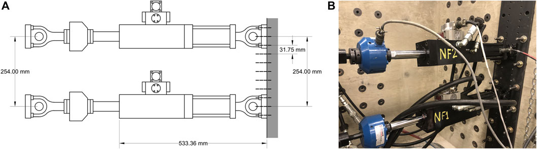
FIGURE 10. Both hydraulic actuators mounted on the strong wall at IISL (A) Drawing (Units: mm), (B) Photograph.

3.4.2 Coupler

The coupler weighs 17.9 kg and is made from SAE 1018 low carbon steel plates. A finite element analysis of this component was performed in Abaqus (Abaqus Unified FEA, 2023) to verify that this coupler will remain below the linear elastic limit of 344.7 N/mm² (50 ksi) for the range of forces and displacements the frame can experience. For example, the application of combination of forces corresponding to the maximum capacity of the hydraulic actuator provides maximum von Mises and principal stresses of 115.9 N/mm² (16.8 ksi) and 135.4 N/mm² (19.6 ksi), respectively. The maximum strain in this set of simulations is 0.0006 mm/mm. Figure 11 illustrates some aspects of this component.

FIGURE 11

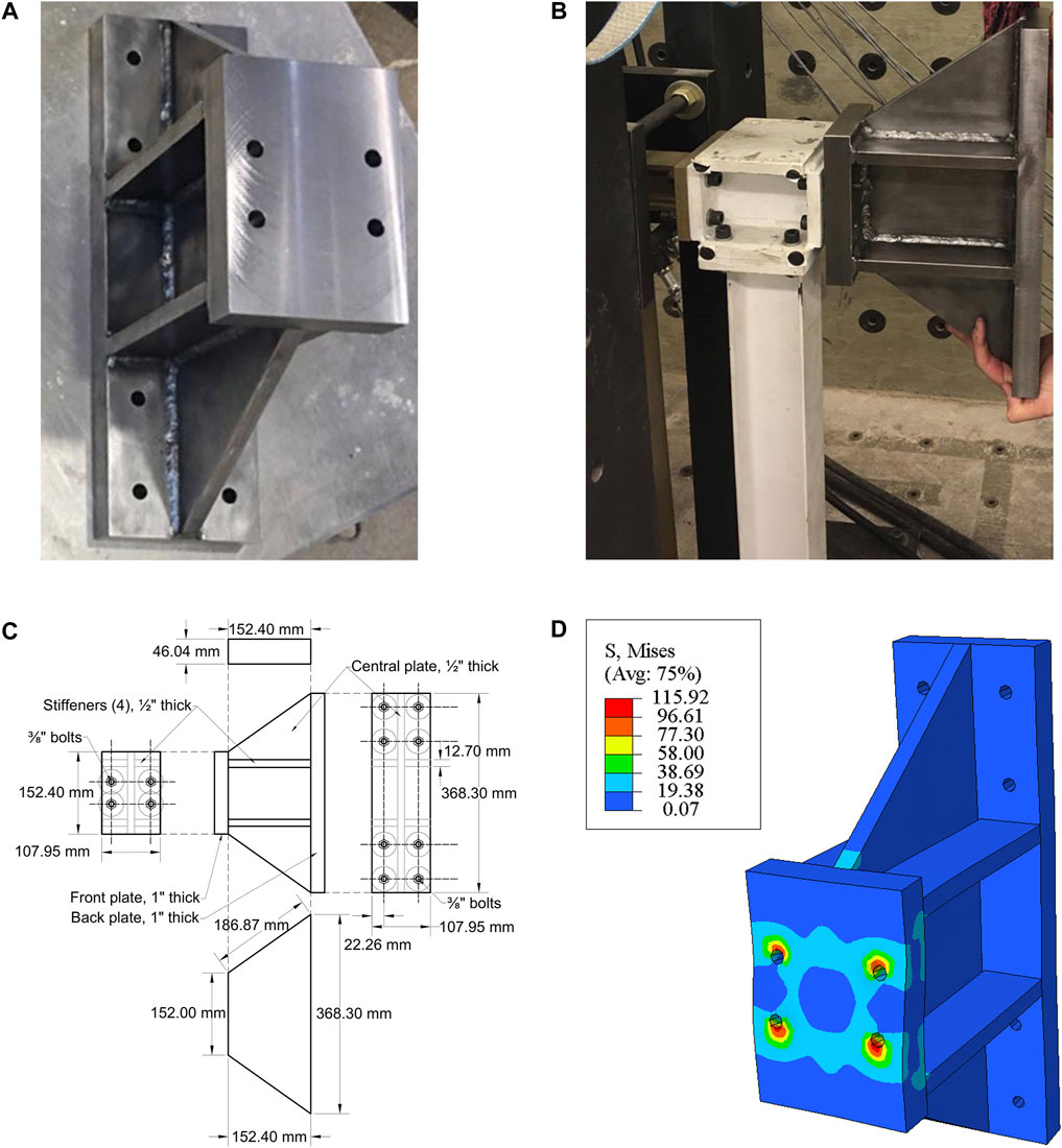
FIGURE 11. Coupler design and implementation. (A) Coupler, (B) Physical implementation of the coupler attached to the frame, (C) Coupler dimensions, (D) Finite element model in ABAQUS: Stress-strain analysis.

In summary, the two hydraulic actuators and coupler form the transfer system for the experimental setup. Due to experimental setup limitations, only the transfer system for node 4 of the experimental substructure is implemented. Figure 12 shows the experimental setup of this transfer system attached to the experimental substructure frame. An additional structure (black frame) prevents motion in the direction perpendicular to the experimental frame plane. This entire setup was assembled in the IISL.

FIGURE 12

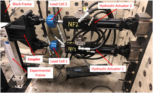
FIGURE 12. Transfer system mounted on our concrete wall and attached to the experimental frame (in white).

3.5 Control problem statement

Since RTHS requires a transfer system to drive the experimental substructure, the dynamics and response of the physical domain are affected by numerous well-known issues such as time delays, frequency-dependent time lags, measurement noise, control-structure interaction (CSI), servo-actuator dynamics, internal coupling in multi-actuator and multi-axial RTHS experiments, environmental and laboratory conditions at the time of the testing, etc. (Dyke et al., 1995; Phillips et al., 2013; Fermandois and Spencer, 2017; Nakata et al., 2023). These effects often play an important role in the accuracy and stability of RTHS, and if they are not considered, the quality of the RTHS can be substantially compromised.

In this regard, a properly designed and tuned control system is typically required to accommodate and compensate for these various issues if the goals of the test itself are to be achieved. The control system typically consists of three elements: 1) the plant to be controlled, which includes the dynamics of the system (structure) plus the transfer system (enforcer of the control action); 2) the sensing system, which comprises of all the required sensors to measure the responses of the plant; 3) a digitally implemented controller that takes the measured response(s) of the plant, estimate the necessary states if required, and generates a control action according to a specific control law. This element typically operates in closed loop, and includes one or more control layers for achieving the desired performance, and estimators for generating unmeasured or noisy states.

A block diagram of the key components described herein is presented in Figure 13A, where the signals and closed loops describe the maRTHS configuration and establish the physical or computational implementation of each component of this maRTHS. Figure 13B shows the experimental implementation of the control plant in the IISL.

FIGURE 13

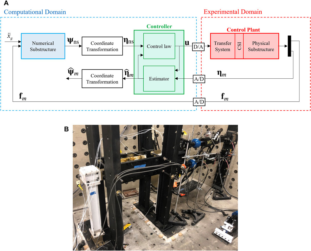
FIGURE 13. maRTHS scheme and control plant implementation in the IISL laboratory. (A) Block diagram of the maRTHS, (B) The control plant.

Meeting the control objectives in this maRTHS scheme is a tracking problem. The main task of this benchmark is to design a control system (see Figure 13) such that the output of the control plant η_m (measured actuator displacements) tracks the target displacement vector η_ns (the response of the numerical substructure in actuator coordinates) and assesses the tracking performance and the overall RTHS performance. The control problem in Figure 13A is simplified in the closed-loop block diagram shown in Figure 14. Participants in this benchmark study will develop and implement their own controllers, following the details to be explained in Section 4. An example of designing and implementing a control scheme, based on a MIMO LQG approach is presented in Section 5.

FIGURE 14

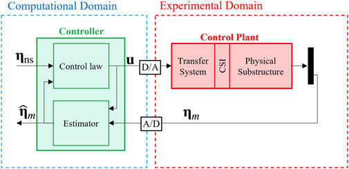
FIGURE 14. Tracking control block diagram.

An estimator is also necessary since the measured signals, ${\mathbf{\eta }}_m$, contain high frequency noise, and not all the states can be measured. Therefore, the state of the physical substructure must be estimated (the high frequency content is filtered out by the estimator). Then the estimated state ${\widehat{\mathbf{\eta }}}_m$ is used by the control law to realize a control input u, which is then sent to the control plant.

In Section 3.4, it was established that a target displacement vector, ${\mathbf{\psi }}_{\text{ns}4}\left[\mathrm{4,28}\right]={\left[x_{\text{ns}4}{\theta }_{\text{ns}4}\right]}^T$, must be imposed to the physical substructure using two hydraulic actuators. Since hydraulic actuators provide translational motion only, a coordinate transformation between “frame coordinates” and “actuator coordinates” is required. Given that the control system must send command signals to the actuators (in actuator coordinates, i.e., linear displacements), the coordinate transformation functions are located between the numerical substructure and the control system, as shown in Figure 13A. Thus, ${\mathbf{\eta }}_m={\left[{\eta }_{m1}{\eta }_{m2}\right]}^T$ is the multi-axial actuator displacement equivalent to the frame node target displacement vector ${\mathbf{\psi }}_{\text{ns}4}\left[\mathrm{4,28}\right]$. Then, the control system realizes the control input vector $\mathbf{u}={\left[u_1{u}_2\right]}^T$, which are commanded to each hydraulic actuator to drive the physical substructure accordingly. Likewise, once the estimator computes the estimated actuator displacement vector ${\widehat{\mathbf{\eta }}}_m={\left[{\widehat{\eta }}_{m1}{\widehat{\eta }}_{m2}\right]}^T$, these actuator coordinates are transformed back to frame coordinates ${\mathbf{\psi }}_{\text{ns}4}\left[\mathrm{4,28}\right]$.

The feedback signal required to satisfy equilibrium conditions at the interface node in the numerical substructure is the experimental force vector ${\mathbf{f}}_{m4}={\left[F_{m4}{M}_{m4}\right]}^T$ , where $F_{m4}$ and $M_{m4}$ are the force and moment corresponding to the degree-of-freedom in the vector ${\mathbf{\psi }}_{\text{ns}4}\left[\mathrm{4,28}\right]$.

Some essential assumptions have been made to define the structure of the control system illustrated in Figure 13B. In principle, the target signal is ${\mathbf{\psi }}_{\text{ns}4}\left[\mathrm{4,28}\right]$, therefore, the controller should take measured translation and rotation ${\mathbf{\psi }}_{\text{es}4}\left[\mathrm{4,28}\right]$ of the experimental frame joint so that a direct tracking error would be evaluated. Nonetheless, measuring these states directly at the joint is difficult. Therefore, considering the mechanical properties of the different components and their behavior, the following assumptions can be stated: first, the frame behavior is linear elastic, which guarantees small deformations and deflections. The coupler has a high stiffness and it can be assumed to be rigid. Likewise, the column-beam joint can be considered rigid (Castaneda, 2012). Finally, the coupler and joint are connected with four high-strength grade 5 bolts with a maximum tensile strength of 827.4 MPa (120 ksi), which is adequate for the range of forces required in this benchmark. These bolts connecting these two components will experience small deformations. Therefore, the strains experienced by the coupler and the column-beam joint are considered negligible, and it can be concluded that by measuring the displacement of the hydraulic actuators through LVDTs, the derived translational and rotational motion at node 4 of the experimental frame can be accurately obtained. In Section 3.7, performance indices ${\mathbf{J}}_2$ and ${\mathbf{J}}_5$ will be developed to quantify any errors produced by our set of assumptions.

3.6 Implementation and constraints

The realization of this maRTHS problem requires the discussion of specific characteristics of its implementation and the definition of certain constraints to reproduce as close as possible actual laboratory conditions.

3.6.1 Physical implementation

An essential characteristic of the behavior of the frame/coupler that has a critical impact on the forces in the hydraulic actuators is due to the deflected shape of the frame when it is pushed or pulled laterally. Figure 15 shows the deflected shape of the frame with the coupler. Due to the rigidity of the column-beam joint, the coupler is forced to rotate as the frame moves laterally. Following this illustration, if each actuator is commanded such that it will move with the same displacement, each actuator would experience different and opposite forces as shown in Figure 16A. Here, if each actuator is pushing the same amount (green arrows), the frame would move to the left causing the coupler to rotate counterclockwise, which would generate a compression effect at the bottom and a tension effect at the top (yellow arrows). Therefore, the net force in the bottom actuator (blue arrow) would be the addition of both effects, and the net force in the top actuator (red arrow) would be the difference of these effects. A similar behavior with inverted force directions occurs when the frame is being pulled.

FIGURE 15

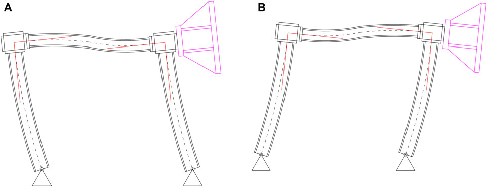
FIGURE 15. Deflected shape of the frame and coupler due to lateral motion. (A) Frame being pushed, (B) Frame being pulled.

FIGURE 16

FIGURE 16. Experimental forces in actuators due to frame deformation. (A) Net forces in actuators due to command displacements to the left (pushing the frame) of equal amplitude, (B) Experimental forces in actuators when the frame is being pushed (positive values indicate compression), (C) Experimental forces in actuators when the frame is being pulled (positive values indicate compression).

To verify this behavior of the actuator-coupler-frame system, an experiment was conducted. A displacement ramp signal of 4 mm is commanded to both actuators to push the frame in one direction. Figure 16B shows the resulting measured forces in each actuator. The bottom actuator experiences the sum of the effect of the pushing actuators plus the compressive effect of the coupler on the actuator due to lateral frame deflection. On the other hand, the top actuator experiences the lateral deflected frame effect, which counteracts the pushing action. In fact, a tension force in the top actuator demonstrates that the deflected frame effect is greater than the pushing force due to the command displacement. Figure 16C shows the case in which the frame is being pulled. From these observations, it can be concluded that the bottom actuator reaches its maximum capacity first under lateral motion regardless of the direction. These characteristics are considered in the experimental configuration to prevent saturation in the actuators, and in the computational domain to properly model the plant and for the design of the control system.

3.6.2 Computational implementation

The computational platform for implementing this benchmark problem is MATLAB/Simulink R2019b (MATLAB, 2023). To conduct the experiment, all models and computational components deployed onto a Speedgoat real-time machine (Performance Real-Time Target Machine, 2023). Thus, the numerical substructure, estimator, control law, and any further necessary modeled components and identified parameters are defined in MATLAB scripts and Simulink models. The structure utilized in this benchmark will be limited to linear elastic behavior, which is achieved because the maximum lateral displacement of the frame is limited to ±4 mm. The mass, damping, and stiffness matrices are extracted to define the reference model, and to partition and numerical substructure according to Section 3. The Newmark’s method integration scheme described in Section 3.2 is implemented to integrate their responses. For designing the control system, an identified model (nominal model) is generated by processing experimental data and is described by a transfer function matrix with target displacements (${\mathbf{\eta }}_{\text{ns}}$) as inputs, and measured displacements (${\mathbf{\eta }}_m$) as outputs. This system is converted into state-space form to facilitate the design of the control system. The Runge-Kutta integration scheme available in Simulink is used for the numerical integration of these systems of first order differential equations. These files are included in the companion tool for executing vRTHS.

3.6.3 Benchmark problem constraints

1. Only displacements and forces of each actuator are available because those measurements may be acquired physically by sensors.

2. If any given proposed control strategy requires additional or higher order states, these must be estimated.

3. Participants may choose to derive their own plant model using the ID experimental data available in the companion package, see Section 4.6. In vRTHS, a plant model replaces the actual experimental plant and a nominal plant model must be used to design the control system. To reproduce more realistic RTHS conditions, the control system must consider the uncertainties in the actual plant.

4. The system-level vRTHS simulation is executed in real-time at a sampling frequency of 1,024 Hz.

5. Each hydraulic actuator has a force capacity of 9340 N and maximum velocity of 25 mm/s. The maximum axial displacements must remain within ±4 mm to guarantee linear elastic behavior of the frame.

6. For acquiring data and outputting commands, an I/O board with 18 bit A/D converters is used. The command inputs must remain within ±4 V. These bounds are implemented with saturation and quantizer blocks in the benchmark code companion package.

7. The conversion relations between the voltage signals and physical units are:

Actuator 1:

Voltage to displacement: 7.4921 mm/V.

Voltage to force: 2074.74 N/V.

Actuator 2:

Voltage to displacement: 7.3907 mm/V.

Voltage to force: 2006.36 N/V.

8. The measured responses contain noise. In the companion tool, these are implemented based on experimental data. The root-mean-square (RMS) values and standard deviation (STD) for these measured signals are:

Actuator 1:

Displacement: RMS = 0.0182 mm, STD = 0.0172 mm.

Force: RMS = 74.40 N, STD = 20.13 N.

Actuator 2:

Displacement: RMS = 0.0199 mm, STD = 0.0198 mm.

Force: RMS = 10.95 N, STD = 7.62 N.

3.7 Evaluation criteria

To assess the overall performance of the maRTHS, the quantitative evaluations consider: 1) tracking control performance (minimize error between target and measured displacements); and 2) global RTHS experiment performance (minimize the error between the reference structure response and the hybrid system response) are required. A set of 10 evaluation criteria is considered in this benchmark. The first six assess the tracking performance of the control system, and the remaining four compute the global performance of the RTHS. These criteria are computed after the RTHS (or vRTHS) is concluded. Table 1 summarizes the indices and briefly describes each criterion. Most of the criteria are evaluated at the interface node at the first story and some are evaluated at upper stories nodes 2 and 3, see Figure 6.

TABLE 1

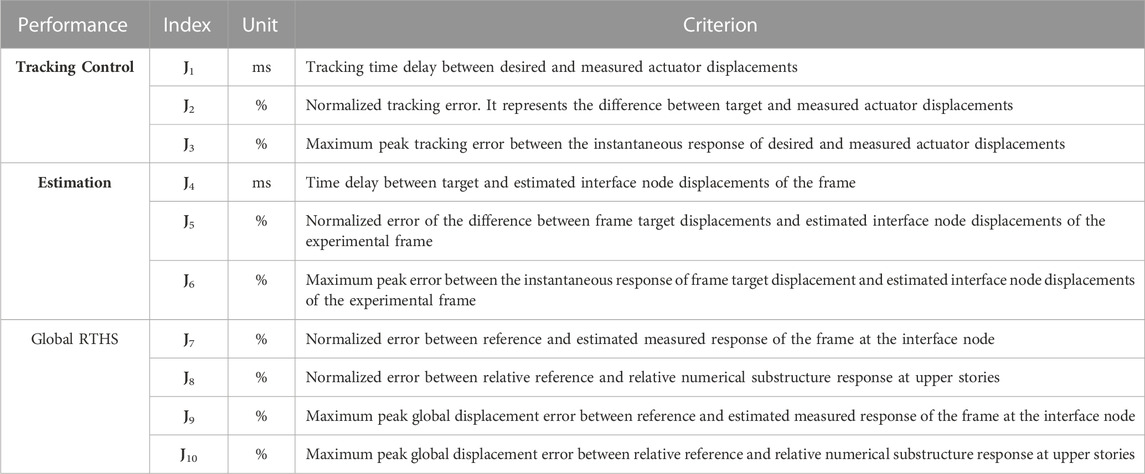
TABLE 1. Criteria for assessment of tracking and global RTHS performance.

Due to the MDOF characteristic of this benchmark, each of the indices in Table 1 are vectors. For instance, the tracking control index ${\mathbf{J}}_2={\left[\begin{array}{cc}{J}_{\mathrm{2,1}}& J_{\mathrm{2,2}}\end{array}\right]}^T$ has two components corresponding to the two hydraulic actuators motion Actuator 1 and Actuator 2, whereas the global performance index for upper stories ${\mathbf{J}}_8={\left[\begin{array}{cc}{J}_{\mathrm{8,2}}& \begin{array}{cc}{J}_{\mathrm{8,26}}& \begin{array}{cc}{J}_{\mathrm{8,3}}& J_{\mathrm{8,27}}\end{array}\end{array}\end{array}\right]}^T$ has four components that represents the translational and rotational DOFs of the second story at node 2 (i.e., ${\psi }_2,{\psi }_{26}$) and of the third story at node 3 (i.e., ${\psi }_3,{\psi }_{27}$). See Figure 3 or 6 for the DOFs definition.

With reference to Figure 13A, it can be useful to recall the notation of the vector components that represent the different responses. The subscript ‘ns’ and ‘m’ stands for “numerical substructure” and “measured,” respectively; when this subscript is absent, the variable represents the reference response (e.g., Eq. (15)). A “hat” over a variable indicates an estimated (or filtered) value. The next subscript (after a comma) represents the position in a vector (e.g., a specific DOF in the relative displacement vector $\mathbf{\psi }$ of the reference frame or a specific actuator displacement in the vector ${\mathbf{\eta }}_m$). The variable ‘k’ in brackets represents the discrete time sequence and ‘N’ is the number of samples in the time series.

3.7.1 Tracking control and estimation: assessment of numerical substructure and the plant responses

J₁—time delay (ms): Estimation of time delay in the controlled response is based on the quantification of the similarity between target and measured displacement time series. The cross correlation between a delayed and target signals provides a sequence that enables the estimation of the number of time steps that the delayed signal has to be shifted so that it provides the maximum correlation with respect to the target signal. Therefore, the arguments of the arg max function of the cross correlation between the actuator target displacement vector and actuator measured displacement vector computes this integer number, which is divided by the sampling frequency (or multiply by the time step) to determine the time delay:

$J_{1,i}=\underset{r}{\arg \max }\left({\displaystyle \sum _{k=1}^N}{\eta }_{\text{ns},i}\left[k\right]\cdot {\eta }_{m,i}\left[k-r\right]\right)\times 1000/f_s,i=\mathrm{1,2},(9)$

where ${\eta }_{m,i}\left[k\right]$ and ${\eta }_{\text{ns},i}\left[k\right]$ are the i-th elements of the vectors ${\mathbf{\eta }}_m={\left[{\eta }_{m,1}{\eta }_{m,2}\right]}^T$ and ${\mathbf{\eta }}_{\text{ns}}={\left[{\eta }_{\text{ns},1}{\eta }_{\text{ns},2}\right]}^T$, respectively at a specific time step k. ${\mathbf{J}}_1={\left[\begin{array}{cc}{J}_{\mathrm{1,1}}& J_{\mathrm{1,2}}\end{array}\right]}^T$ contains the indices for the two actuators; $f_s$ is the sampling frequency.

J₂—tracking error (%): This index processes the normalized root mean square (NRMS) of the error between the actuator target displacement vector and the actuator measured displacement vector:

$J_{2,i}=\sqrt{\frac{\sum _{k=1}^N{\left({\eta }_{m,i}\left[k\right]-{\eta }_{\text{ns},i}\left[k\right]\right)}^2}{\sum _{k=1}^N{\left({\eta }_{\text{ns},i}\left[k\right]\right)}^2}}\times 100,i=\mathrm{1,2}.(10)$

J₃—peak tracking error (%): This index computes the maximum relative error between the actuator target displacement vector and the actuator measured displacement vector:

$J_{3,i}=\frac{\max \left(\left|{\eta }_{m,i}\left[k\right]-{\eta }_{\text{ns},i}\left[k\right]\right|\right)}{\max \left(\left|{\eta }_{\text{ns},i}\left[k\right]\right|\right)}\times 100,i=\mathrm{1,2}.(11)$

J₄—time delay of estimated response (ms): Similar to ${\mathbf{J}}_1$, this index assesses the time delay between the actuator target displacement vector, ${\mathbf{\eta }}_{\text{ns}}$, and the actuator estimated displacement vector, ${\widehat{\mathbf{\eta }}}_m$.

$J_{4,i}=\underset{r}{\arg \max }\left({\displaystyle \sum _{k=1}^N}{\eta }_{\text{ns},i}\left[k\right]\cdot {\widehat{\eta }}_{m,i}\left[k-r\right]\right)\times 1000/f_s,i=\mathrm{1,2},(12)$

J₅—estimation error (%): This index considers the NRMS of the error between the target displacement vector and the estimated measured displacement vector at the interface node of the frame (node 4, see Figure 6):

$J_{5,i}=\sqrt{\frac{\sum _{k=1}^N{\left({\widehat{\psi }}_{m,i}\left[k\right]-{\psi }_{\text{ns},i}\left[k\right]\right)}^2}{\sum _{k=1}^N{\left({\psi }_{\text{ns},i}\left[k\right]\right)}^2}}\times 100,i=\mathrm{4,28},(13)$

where ${\widehat{\psi }}_{m,i}$ and ${\psi }_{\text{ns},i}$ represent the estimated measured response and the target displacement (numerical substructure response) of the i-th DOF of the FE model at a specific time step k. See Figure 6.

The difference between indices ${\mathbf{J}}_5$ and ${\mathbf{J}}_2$ when ${\eta }_{m,i}\left[k\right]$ is replaced by ${\widehat{\eta }}_{m,i}\left[k\right]$ in Eq. (10) represents to some extent the error due to the assumptions described in Sections 3.5 and 4.3.

J₆—peak estimation error (%): This index computes the maximum relative error between the target displacement vector and the estimated measured displacement vector at the interface node of the frame:

$J_{6,i}=\frac{\max \left(\left|{\widehat{\psi }}_{m,i}\left[k\right]-{\psi }_{\text{ns},i}\left[k\right]\right|\right)}{\max \left(\left|{\psi }_{\text{ns},i}\left[k\right]\right|\right)}\times 100,i=\mathrm{4,28}.(14)$

3.7.2 Global performance: assessment of the RTHS response with respect to the reference structure

J₇—global response error at interface node (%): This index assesses the difference between the response of the reference structure and the hybrid system (vRTHS or RTHS). It computes the NMRS error between the reference response and the estimated measured response of the frame at the node interface.

$J_{7,i}=\sqrt{\frac{\sum _{k=1}^N{\left({\widehat{\psi }}_{m,i}\left[k\right]-{\psi }_i\left[k\right]\right)}^2}{\sum _{k=1}^N{\left({\psi }_i\left[k\right]\right)}^2}}\times 100,i=\mathrm{4,28},(15)$

where ${\psi }_i\left[k\right]$ represent the reference response corresponding to the i-th DOF of the reference model.

J₈—global relative response error at upper stories (%): The response errors in the upper stories are evaluated by considering nodes 2 and 3 of the frame model, see Figure 6. Therefore, the NMRS error is calculated between the relative response of the reference structure and numerical substructure at their respective nodes for the translational and rotational DOF, x and θ.

$J_{8,i}=\sqrt{\frac{\sum _{k=1}^N{\left({\psi }_{\text{ns},i}\left[k\right]-{\psi }_i\left[k\right]\right)}^2}{\sum _{k=1}^N{\left({\psi }_i\left[k\right]\right)}^2}}\times 100,i=\mathrm{2,26,3,27}.(16)$

J₉—peak global response error at interface node (%): This index evaluates the maximum error between the reference response and the estimated measured response at the interface node of the frame:

$J_{9,i}=\frac{\max \left(\left|{\widehat{\psi }}_{m,i}\left[k\right]-{\psi }_i\left[k\right]\right|\right)}{\max \left(\left|{\psi }_i\left[k\right]\right|\right)}\times 100,i=\mathrm{4,28}.(17)$

J₁₀—peak global response error at upper stories (%): This index computes the maximum error between the relative displacement of the reference structure and numerical substructure at nodes of the frame:

$J_{10,i}=\frac{\max \left(\left|{\widehat{\psi }}_{\text{ns},i}\left[k\right]-{\psi }_i\left[k\right]\right|\right)}{\max \left(\left|{\psi }_i\left[k\right]\right|\right)}\times 100,i=\mathrm{2,26,3,27}.(18)$

4 Virtual maRTHS (vmaRTHS) implementation

A realistic vmaRTHS code package is established for participants to evaluate their controllers in a modular fashion. The scripts and other resources containing models and data are discussed in the sequel.

4.1 Overview

This vRTHS tool is implemented using scripts and block models in MATLAB/Simulink R2019b, respectively. This virtual implementation is as close as possible to RTHS. The companion package includes a Starting_Guideline.pdf file that explains how to work with the code. Figure 17 shows the basic organization of the code package. The top-level folder has three files only:

• A guideline document: Starting_Guideline.pdf

• A main script: main_vmaRTHS.m

• A block model: Model_vmaRTHS_R2019b.slx

FIGURE 17

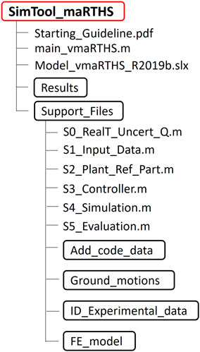
FIGURE 17. File organization of the companion package.

Additional folders contain experimental data for identification of the plant, input data, ground motions, finite element model of the reference structure, and necessary scripts such as functions for defining and loading different components of the vmaRTHS. The main script main_vmaRTHS.m is in charge of initialization, loading models and control system, running the vmaRTHS, assessment of the results, and it is the only script that needs to be executed to run this tool. The files the participants must modify are the script S3_Controller.m and the corresponding control block in the Simulink model.

Figure 18 shows the execution flow of the principal files (scripts and block models) involved in this implementation as well as their related formulations. The user defines the control system and has the choice, based upon the specific features of the control scheme to be used, of developing its own nominal plant model with the experimental data for identification that is available or use the nominal plant provided as an example in this benchmark. With control design in mind, this tool can also be executed offline.

FIGURE 18

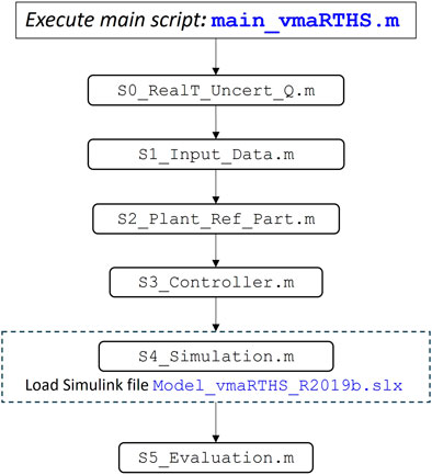
FIGURE 18. Flow diagram.

4.2 Control plant model

The control plant defined in Section 3.5 has two inputs ${\left[u_1{u}_2\right]}^T$ and two outputs ${\left[{\eta }_{m,1}{\eta }_{m,2}\right]}^T$ representing the control inputs and the hydraulic actuator displacements, respectively. According to Figures 8, 9, subscript 1 represents the bottom actuator and 2 represents the top actuator. Therefore, a compact 2 × 2 matrix description of the control plant is convenient. Eq. (19) shows a mathematical representation of the control plant in terms of a transfer function matrix.

$\mathbf{H}=\left[\begin{array}{cc}{H}_{11}& H_{12}\\ H_{21}& H_{22}\end{array}\right],(19)$

where $H_{ij}$ is the transfer function from input j to output i. The diagonal terms describe the direct relationship between the input and output of a specific actuator when this is commanded, whereas the off-diagonal terms provide the internal coupling behavior of one actuator when the other is commanded.

Since the frame contains component that are all part of one dynamic system, its poles should be common in Eq. 19 and the remaining poles of the system will depend on the model of the transfer system. Therefore, Eq. (19) can be written as

$\mathbf{H}=\left[\begin{array}{cc}\frac{{num}_{11}\left(s\right)}{{den}_{11}\left(s\right)}& \frac{{num}_{12}\left(s\right)}{{den}_{12}\left(s\right)}\\ \frac{{num}_{21}\left(s\right)}{{den}_{21}\left(s\right)}& \frac{{num}_{22}\left(s\right)}{{den}_{22}\left(s\right)}\end{array}\right]\cdot \frac{{num}_{\text{es}}\left(s\right)}{{den}_{\text{es}}\left(s\right)},(20)$

where ${num}_{ij}\left(s\right)/{den}_{ij}\left(s\right)$ represents the numerator and denominator of the transfer function $H_{ij}$ and ${num}_{\text{es}}\left(s\right)/{den}_{\text{es}}\left(s\right)$ characterizes the poles and zeros of the frame (experimental substructure).

4.3 Coupler coordinate transformation

The use of two hydraulic actuators to enforce translation and rotation requires a coordinate transformation between the degrees of freedom of the numerical substructure and the two actuator displacements. Four assumptions are made to develop this relation: 1) the coupler deformations are negligible. The analysis presented in Section 3.4 demonstrates that the maximum strains in the coupler justify this assumption; 2) the vertical motion of the nodes can be neglected. The axial deformation of the columns in the physical substructure is negligible due to their high axial stiffness, and the axial forces in the columns are small since the motion of the frame is mainly horizontal; 3) the rotations of the column-beam joints are small because the behavior of the frame in this benchmark is limited to linear elastic; 4) the connection of the coupler to the column-beam joint provided by the high-strength bolts is rigid, hence the deformations are negligible.

Therefore, the coupler can be considered as a rigid body, the boundary conditions of the coupler at the column-beam joint allows two degrees of freedom, and the kinematics of the actuators can be described entirely by the horizontal components of their motion. Figure 19A shows that the model of the coupler is defined by the rigid triangle AOB. The vertex $O_f$ is located at the intersection of the beam and column axes, and vertices A and B represent the location where the hydraulic actuators are attached.

FIGURE 19

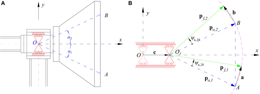
FIGURE 19. Coupler modeled as a rigid body. (A) Rigid body geometry, (B) Rigid body motion.

Figure 19B illustrates the motion of the coupler (initial position in blue and final position in green) and the corresponding attached actuators trajectories when the frame moves laterally. The actuators axial displacements can be obtained by adding the effect of the horizontal displacement of the coupler $\mathbf{c}$ (translational DOF of node 4, ${\psi }_{\text{ns}\mathrm{4,4}}$, imposed on the physical frame) and the horizontal components of the vectors $\mathbf{a}$ and $\mathbf{b}$ when the coupler rotates the angle ${\psi }_{\text{ns}\mathrm{4,28}}$. For instance, considering the rotation effect only, the initial position of the top actuator can be represented by the vector ${\mathbf{p}}_{o,2}$ and its final position by the vector ${\mathbf{p}}_{f,2}={\mathbf{p}}_{o,2}+\mathbf{b}$. Thus, the actuator axial displacements can be written as:

${\mathit{\eta }}_{m,i}=\mathbf{c}+{\mathbf{p}}_{f,i}-{\mathbf{p}}_{o,i},i=\mathrm{1,2}(21)$

and its magnitude can be approximated by its horizontal component:

${\eta }_{m,i}={\psi }_{m,4}+p\cdot \left[\cos \left({\alpha }_i+{\psi }_{m,28}\right)-\cos \left({\alpha }_i\right)\right].i=\mathrm{1,2}(22)$

Where $p=\left|{\mathbf{p}}_{o,i}\right|=\left|{\mathbf{p}}_{f,i}\right|$ since the coupler is assumed to be rigid. The inverse relation is:

${\psi }_{m,28}={\sin }^{-1}\left(\frac{{\eta }_{m,1}-{\eta }_{m,2}}{2p\sin \left({\alpha }_2\right)}\right)(23)$

and

${\psi }_{m,4}={\eta }_{m,i}-p\cdot \left[\cos \left({\alpha }_i+{\psi }_{m,28}\right)-\cos \left({\alpha }_i\right)\right].(24)$

4.4 Control plant uncertainties

Actual uncertainties in the plant such as imprecision in the size of elements, material properties, parameters, etc. and a simplified representation of the plant’s dynamics yield to model imprecision. Therefore, it is realistic to incorporate uncertainties into the control plant used in this benchmark so that the proposed control approach is tested realistically as well via virtual RTHS.

$\mathbf{H}=\left[\begin{array}{c}2165.2\frac{\left(s+120\right)\left(s+90\right)}{\left(s+2.65\right)\left(s+40\right)}4.5e6\frac{\left(s+3\right)}{\left(s+3.5\right)\left(s+18.5\right)}\\ 349.95\frac{\left(s+120\right)\left(s+90\right)}{\left(s+2.65\right)\left(s+40\right)}2165.2\frac{\left(s+5\right)}{\left(s+3.5\right)\left(s+18.5\right)}\end{array}\right]\cdot \frac{{num}_{\text{es}}\left(s\right)}{{den}_{\text{es}}\left(s\right)},(25)$

This benchmark problem considers uncertainties or model inaccuracies in the control plant by defining random variations in the transfer function matrix of a nominal plant model that has the form of Eq. (20). Random variations in the poles and zeros of the nominal plant model generate these differences by introducing changes from a standard normal distribution sampling process, which create a family of frequency response functions (FRF) where any FRF member represents a potential control plant. Table 2 presents the mean and standard deviation for each of these poles and zeros of the nominal plant model that can be described by Eqs 19, 20. In this benchmark, and commonly in practice, the nominal plant model is an identified plant model that is provided in the companion package tool.

$\frac{{num}_{\text{es}}\left(s\right)}{{den}_{\text{es}}\left(s\right)}=\frac{1}{\left(s+50+63j\right)\left(s+50-63j\right)}.(26)$

TABLE 2

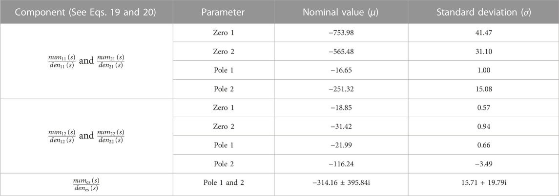
TABLE 2. Parameter uncertainty definition.

Figure 20 shows a set of FRFs generated using the parameters of Table 2 that captures the uncertainty in modeling the control plant. To simulate an actual RTHS experiment, the proposed controller is designed considering an identified plant model (the nominal plant model in this benchmark). Then, a virtual RTHS is conducted where the designed controller tracks a control plant model randomly selected from the FRF family shown in Figure 20. To guarantee robust performance and stability of the controller, at least 20 virtual RTHS should be executed, each one with a randomly selected control plant model. The companion package tool implements these procedures and facilitates the processing of performance metrics data.

FIGURE 20

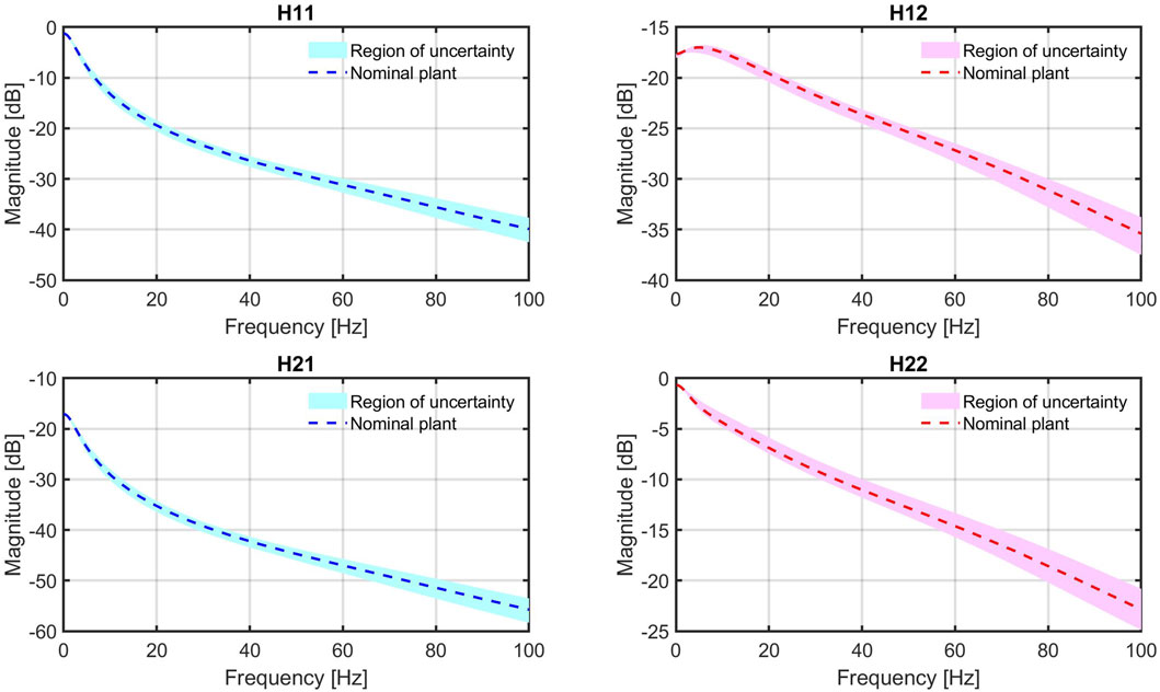
FIGURE 20. FRF regions for the plant model uncertainty.

4.5 Provided materials

This benchmark includes a companion package that helps to implement the control system using vRTHS.

1.Models:

a.Reference model: definition and implementation of a 38-DOF finite element model (M, C, K, see Section 2).

b.Nominal model of the experimental frame: definition and implementation of an 8-DOF finite element model (${\mathbf{M}}_{\text{es}}$, ${\mathbf{C}}_{\text{es}}$, ${\mathbf{K}}_{\text{es}}$, see Section 3.2).

c.Reduced nominal model of the experimental frame: 2-DOF model.

d.Nominal plant model: an identified transfer function matrix of the transfer system, frame, and CSI (Sections 4.2, 4.3).

e.Control plant model with uncertainties: See Section 4.4.

2.Experimental data for identification of the plant: Band-limited white noise (BLWN) input-output data is available. The participants have the flexibility of generating their own models if needed.

3.Input data: For RTHS execution, a set of three unscaled historic ground acceleration records: El Centro 1940, Kobe 1995, and Morgan Hill 1984. For tracking control assessments, chirp and BLWN signals are suggested.

4.Sample control system - LQG control strategy: a control law based on a linear quadratic regulator (LQR) approach and a Kalman estimator.

5.Virtual RTHS code package: This tool contains MATLAB scripts, a Simulink model containing all the components shown in Figure 13B, and data sets. A guideline explains the usage of these files.

All files will be available on the MECHS website: https://mechs.designsafe-ci.org/

4.6 Deliverables

The participants are asked to produce the following to address the benchmark problem:

4.6.1 Tracking control system

The participants have complete freedom to implement control strategies to meet the constraints discussed in Section 3.6. If a specific control approach requires the use of a nominal model different than the provided in the companion package, the participant should explain the formulation and implementation of their particular nominal model.

4.6.2 Generation scripts and Simulink model

A set of MATLAB scripts and Simulink models are required that are compatible with the code package. They must execute in real-time since the ultimate goal is to test the proposed tracking control systems in the IISL laboratory.

4.6.3 Tracking performance evaluation

The indices ${\mathbf{J}}_1$—${\mathbf{J}}_6$ explained in Section 3.7 will assess the tracking control performance of the proposed control system. A set of 10 simulations is required to produce numerical values for these indices.

4.6.4 Overall RTHS performance evaluation

The indices ${\mathbf{J}}_7$—${\mathbf{J}}_{10}$ from Section 3.7 evaluate the overall performance of the hybrid system considering the reference structure as the baseline case. A set of 10 simulations will generate a quantitative evaluation of the global performance.

4.6.5 Comparison plots

Participants are encouraged to generate plots for qualitative evaluation of the performance of their controllers.

5 Example implementation: maRTHS

In this section, a sample of a maRTHS implementation is described. This section especially focuses on presenting an identified control plant and control system realization. The evaluation of the sample design is illustrated according to the evaluation criteria in Section 3. Both numerical and experimental results are provided.

5.1 Identified control plant and coupler dynamics

The high degree of internal coupling in this maRTHS sample demands a systematic procedure to analyze the control plant to obtain the necessary information for system identification. Experimental data was obtained using four energy levels of BLWN signals to the control plant. A first test was conducted using a 0–100 Hz BLWN signal input to the bottom actuator while the other was set to zero displacement and the displacement of both actuators were measured. This set of inputs and outputs was used to compute the experimental transfer functions of the plant, which is the first column of Eq. (19). Likewise, in another test the same signal was used as input to the top actuator while sending a zero to the bottom actuator to generate the second column of the experimental transfer function matrix.

To provide a basic but meaningful nominal model of the control plant, the experimental frame is considered as a 1-DOF second order system with a complex conjugate pair of poles. Even though the hydraulic actuators are of the same model from the manufacturer, they have slightly different behavior in an experimental setup and these dominate each of the columns of the system transfer functions. Thus, a different set of poles is identified for each actuator. The number and type of poles for each system are assumed according to a parametric model previously investigated. The models of the servo-valve and hydraulic dynamics of each actuator are assumed to be represented by first order differential equations (Maghareh et al., 2018). Consequently, in this sample, each actuator is modeled using two real poles. The bandwidth used for this identification process is 40 Hz since the frequencies of interest such as the input signal (ground motion record) and useful natural frequencies of the structure are well below this limit (see Section 2.2). Then, a model with two real poles is fitted to the experimental FRF, see Figure 21. Eqs 25 and 26 describe the identified model of the control plant.

FIGURE 21

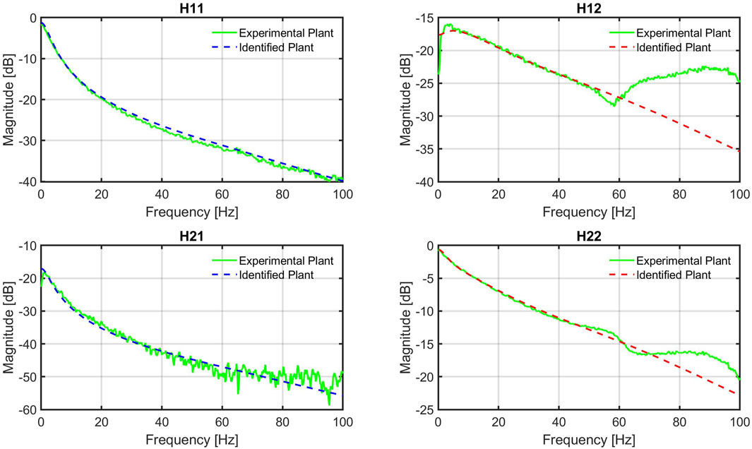
FIGURE 21. Control plant identification: Identified plant FRFs vs. experimental plant FRFs.

Here, ${num}_{\text{es}}\left(s\right)/{den}_{\text{es}}\left(s\right)$ is the transfer function that represents the behavior of the experimental frame. This system is then transformed to state-space form as

$\dot{\mathbf{z}}=\mathbf{A}\cdot \mathbf{z}+\mathbf{B}\cdot \mathbf{u}{\mathrm{\eta }}_m=\mathbf{C}\cdot \mathbf{z}+\mathbf{D}\cdot \mathbf{u},(27)$

where the command displacement vector $\mathbf{u}$ is the input to the system; $\mathbf{z}$ contains the states of the identified control plant; A, B, C, and D are typical constant matrices in state-space description; and the measured actuator displacement vector, ${\mathbf{\eta }}_m$, is the output vector.

5.1.1 Coordinate transformation

In this benchmark, the coupler kinematics may be obtained by applying the geometry of the coupler in Eqs 21–24 with $p=295.39\text{\hspace{0.17em}mm}$ and $\alpha =25.46°$, see Figure 19. Hence, the transform relation from frame to actuator coordinates is given by Eq. 28 and the coordinate transform from actuator to frame is provided by Eqs 29, 30 (see Figure 13B or 22(a) for references).

$\left[\begin{array}{c}{\eta }_{\text{ns},1}\\ {\eta }_{\text{ns},2}\end{array}\right]={\psi }_{\text{ns},4}\left[\begin{array}{c}1\\ 1\end{array}\right]+295.39\left[\begin{array}{c}\cos \left({\psi }_{\text{ns},28}-25.46\frac{\pi }{180}\right)-\cos \left(-25.46\frac{\pi }{180}\right)\\ \cos \left({\psi }_{\text{ns},28}+25.46\frac{\pi }{180}\right)-\cos \left(25.46\frac{\pi }{180}\right)\end{array}\right],(28)$

${\widehat{\psi }}_{m,28}={\sin }^{-1}\left[\frac{{\eta }_{m,1}-{\eta }_{m,2}}{2\times 295.39\sin \left(25.46\frac{\pi }{180}\right)}\right],(29)$

${\widehat{\psi }}_{m,4}={\eta }_{\text{ns},1}-295.39\left[\cos \left({\widehat{\psi }}_{m,28}-25.46\frac{\pi }{180}\right)-\cos \left(25.46\frac{\pi }{180}\right)\right].(30)$

5.2 Feedback force estimation

The RTHS scheme presented in Figure 13B shows the feedback force being measured directly from the control plant, which is typical in RTHS experiments. Despite having load cells available while executing this maRTHS sample in the IISL, it would not be correct to use these measured forces directly. These measurements contain very large inertial forces associated with the coupler, which is not part of the original structural system (the whole frame). Thus, the force that is developed only by the frame must be estimated.

This sample shows a practical approach that uses the FE model of the experimental substructure discussed in Section 3.3. The estimated frame response ${\widehat{\mathbf{\psi }}}_m$ is differentiated twice to obtain its corresponding velocity and acceleration and, similar to Eq. (7), the feedback force would be given by Eq. (31). This implementation is shown in Figure 22A.

${\widehat{\mathbf{f}}}_m={\mathbf{M}}_{\text{es}}\cdot {\widehat{\ddot{\mathbf{\psi }}}}_m+{\mathbf{C}}_{\text{es}}\cdot {\widehat{\dot{\mathbf{\psi }}}}_m+{\mathbf{K}}_{\text{es}}\cdot {\widehat{\mathbf{\psi }}}_m.(31)$

FIGURE 22

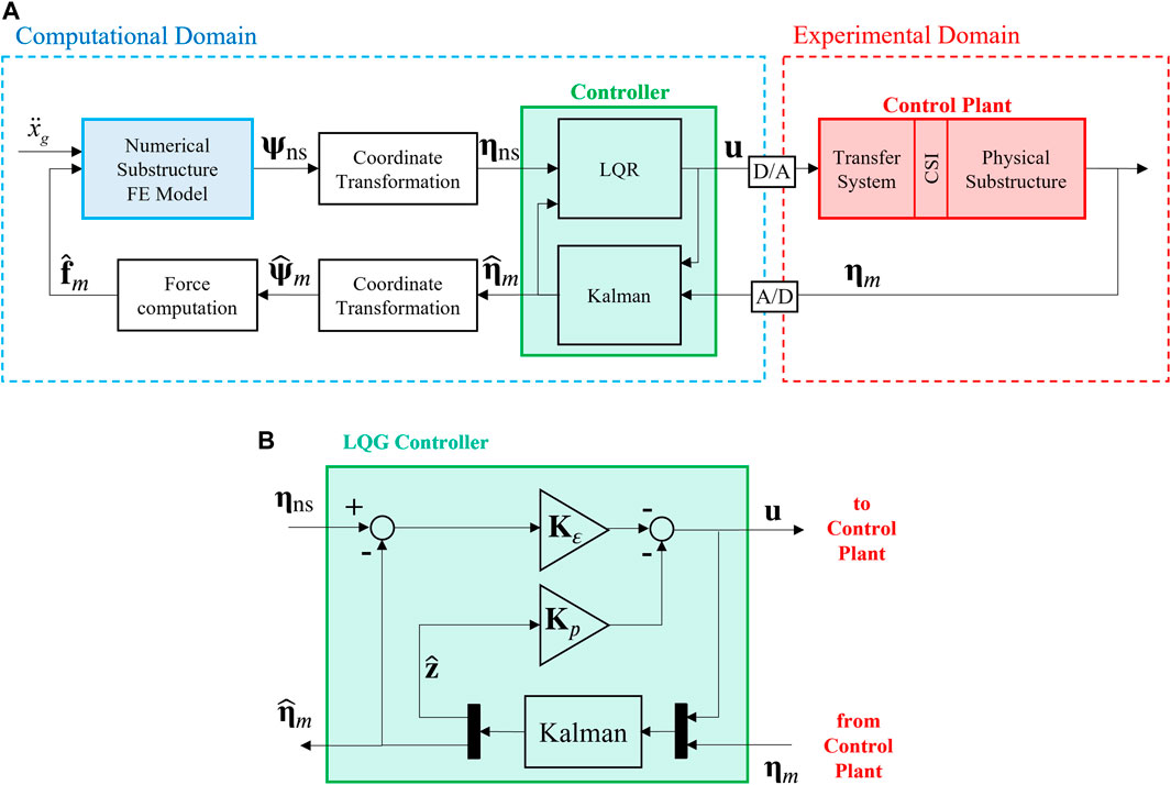
FIGURE 22. maRTHS and control approach implementation. (A) maRTHS implementation, (B) Tracking control and estimation scheme.

The code for this implementation is included in the companion package. Participants can use the identified model developed in this section, which is also available in the companion package, or choose another model based on a preferred methodology.

5.3 Control system: LQG

Among the vast variety of control methodologies feasible for RTHS, this sample is based on an optimal control strategy that is not intended to be competitive. This approach is selected here because it has acceptable performance and at the same time is simple enough to focus on the important features of this maRTHS while overcoming the control requirements and challenges from a hybrid simulation perspective. An LQG control scheme is chosen due to its versatility in introducing uncertainty in state-space form as added noise.

The LQG controller consists of two components in closed loop: (1) a deterministic LQR which assumes full state feedback, and (2) a Kalman filter that estimates the required states to be fed back to the LQR control law. The strategy for including the target signal ${\mathbf{\eta }}_{\text{ns}}$ is to incorporate the error $\mathbf{\epsilon }={\mathbf{\eta }}_{\text{ns}}-{\mathbf{\eta }}_m$ by augmenting and additional state ${\dot{\mathbf{z}}}_{err}=\mathbf{\epsilon }$, and find the optimal gain for the augmented plant, Eq. (32). The trade-off between performance and control effort is defined by selecting appropriate ratios for the weighting matrices Q and R, to minimize the cost function established by Eq. (34). Finally, one solves for the gains required to drive the error state to zero. Thus, the control law, u, is computed with Eq. (35). The MATLAB function ‘lqr’ with matrices ${\mathbf{A}}_a$, ${\mathbf{B}}_a$, Q, and R, provides the gains ${\mathbf{K}}_p$ and ${\mathbf{K}}_{\epsilon }$ to realize the control input u.

${\dot{\mathbf{z}}}_a={\mathbf{A}}_a{\mathbf{z}}_{\mathit{a}}+{\mathbf{B}}_a\mathbf{u}+\mathbf{H}{\mathbf{\eta }}_{\text{ns}},(32)$

where:

${\mathbf{z}}_a=\left[\begin{array}{c}\mathbf{z}\\ {\mathbf{z}}_{err}\end{array}\right],{\mathbf{A}}_a=\left[\begin{array}{cc}\mathbf{A}& \mathbf{0}\\ -\mathbf{C}& \mathbf{0}\end{array}\right],{\mathbf{B}}_a=\left[\begin{array}{c}\mathbf{B}\\ \mathbf{0}\end{array}\right],\mathbf{H}=\left[\begin{array}{c}\mathbf{0}\\ \mathbf{1}\end{array}\right](33)$

$J={\displaystyle \underset{0}{\overset{\infty }{\int }}}\left({\mathbf{z}}_a^T\cdot \mathbf{Q}\cdot {\mathbf{z}}_a+{\mathbf{u}}^T\cdot \mathbf{R}\cdot \mathbf{u}\right)(34)$

$\mathbf{u}=\left[\begin{array}{cc}-{\mathbf{K}}_p& -{\mathbf{K}}_{\epsilon }\end{array}\right]\left[\begin{array}{c}\mathbf{z}\\ \mathbf{\epsilon }\end{array}\right](35)$

However, in this maRTHS experiment the states, z, are not available, i.e., the only measurements available are the measured displacements of the actuators, ${\mathbf{\eta }}_m$. Therefore, estimation of states is necessary to feed them to the control law (Eq. (35)). A Kalman filter is used to overcome this limitation by providing estimated states $\widehat{\mathbf{z}}$ and filtered response ${\widehat{\mathbf{\eta }}}_m$ so that the control system is implemented as shown in Figure 22B. Considering that the process noise and measurement noise covariance matrices are additive with known distributions, Eq. (27) can be written as

$\dot{\mathbf{z}}=\mathbf{A}\cdot \mathbf{z}+\mathbf{B}\cdot \mathbf{u}+{\mathbf{w}}_k{\mathbf{\eta }}_m=\mathbf{C}\cdot \mathbf{z}+\mathbf{D}\cdot \mathbf{u}+{\mathbf{v}}_k(36)$

where the distribution of the process noise is assumed to be ${\mathbf{w}}_k\sim N\left(\mathbf{0},\mathbf{Q}\right)$, and the distribution of the measurement noise is assumed to be ${\mathbf{v}}_k\sim N\left(\mathbf{0},\mathbf{R}\right).$

The final values for Q, R and the Kalman estimator terms can be found in the companion package.

5.4 Experimental results and evaluation

The following figures and table present a qualitative and quantitative assessment of the performance of the sample LQG control system on the maRTHS based on experimental results. The input to the reference and hybrid system for this example is the El Centro earthquake historic record with a scaling factor of 0.40. See Section 4.5 for additional ground motion records. Figures 23–25 shows qualitatively the tracking and global RTHS performance of the interface node (node 4 in Figure 5), while Table 3 presents the metrics defined by the performance indices (see Section 3.7) which includes not only the interface node information, but also additional nodes at the upper stories of the frame for a more comprehensive evaluation of the RTHS.

FIGURE 23

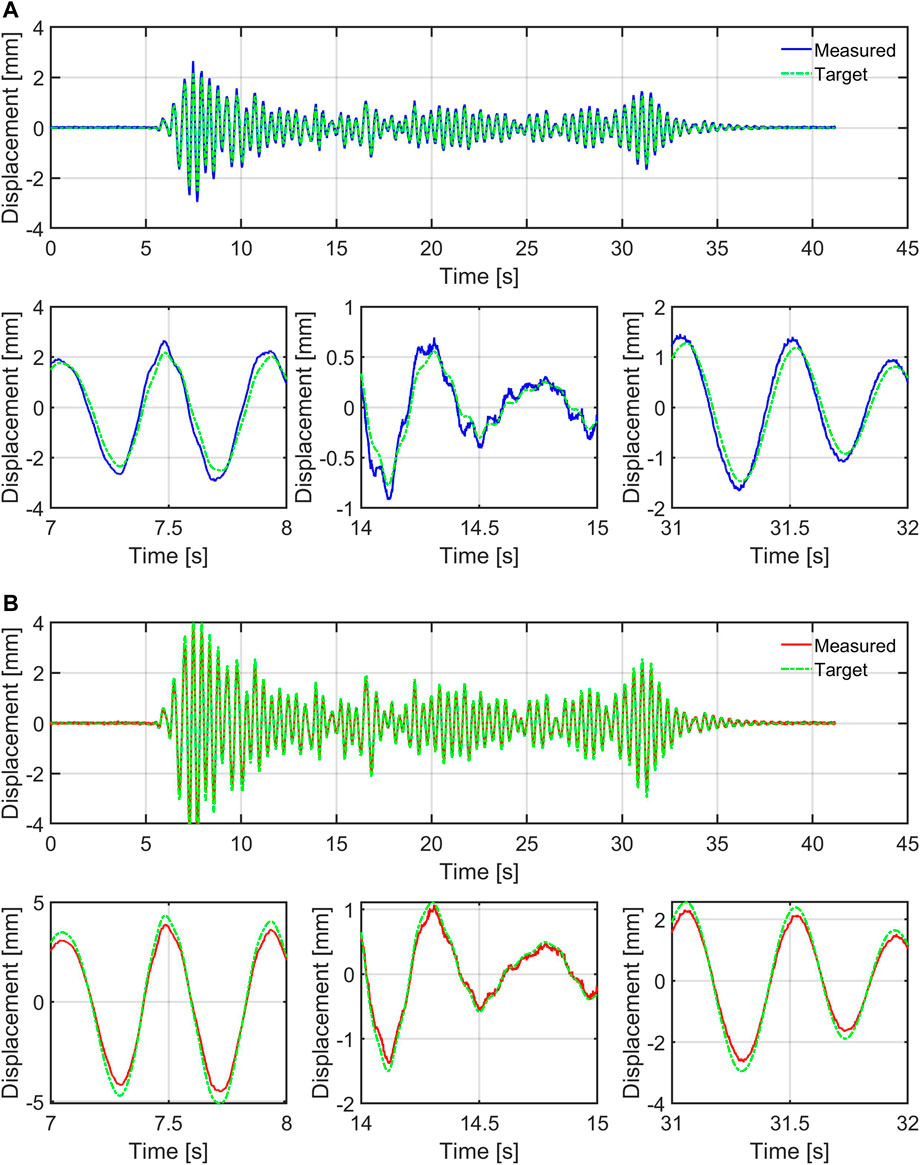
FIGURE 23. maRTHS tracking performance in actuator coordinates. (A) Tracking actuator 1: Target and measured actuator displacements, (B) Tracking actuator 2: Target and measured actuator displacements.

FIGURE 24

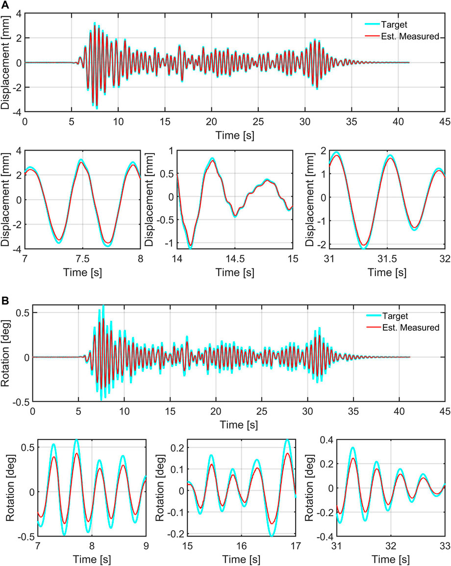
FIGURE 24. maRTHS tracking performance at the interface node (frame coordinates). (A) Tracking of translational DOF: Target numerical substructure vs estimated experimental responses, (B) Tracking of rotational DOF: Target numerical substructure vs estimated experimental responses.

FIGURE 25

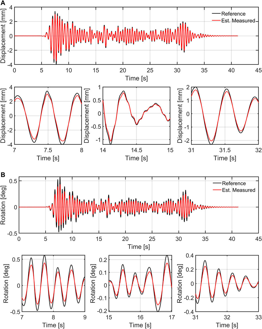
FIGURE 25. maRTHS global performance. (A) Translational DOF: Reference vs estimated experimental response (DOF ψ₄), (B) Rotational DOF: Reference vs estimated experimental response (DOF ψ₂₈).

TABLE 3

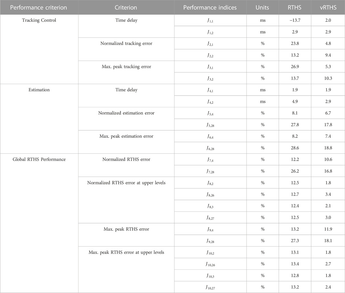
TABLE 3. RTHS and vRTHS evaluation indices.

Figure 23 shows the tracking performance by comparing the measured actuator displacements (${\mathbf{\eta }}_m$) and the target actuator displacements (${\mathbf{\eta }}_{\text{ns}}$) computed from the numerical substructure node displacements. The results show a NRMS error of 23.8% for actuator 1 (bottom) and 13.2% for actuator 2 (top). These results are in agreement with the mechanics explained in Section 3.6: Actuator 1 is counteracted by the deformed frame effect. Conversely, Actuator 2 is “helped” by the same frame effect. From a control perspective, the effort required by actuator 1 to drive the motion of the frame node is greater. This particular behavior of the plant requires the selection of larger Q/R ratios for actuator 1 in the sample LQG controller. If the estimated measured actuator displacements (${\widehat{\mathbf{\eta }}}_m$) are considered, the NRMS tracking errors are 3.2% and 13% for Actuator 1 and Actuator 2, respectively. This result shows the benefits of estimators to enhance the tracking control performance. Despite that the actuator displacements provides direct measurements for tracking assessment, a more realistic evaluation of tracking performance is achieved by considering frame coordinates, i.e., the frame node motion. Figure 24 illustrates a comparison between the transformed (estimated) measured displacement vector ${\widehat{\mathbf{\psi }}}_m$ and the target displacement vector ${\mathbf{\psi }}_{\text{ns}}$ at the interface node. The NRMS error for the translational and rotational DOF are 8.1% and 27.8%, respectively. The increased errors result from the assumptions described in Section 4.3, specifically, the effectiveness of the connection of the coupler to the joint frame, which demonstrates the challenges and limitation in enforcing rotational boundary conditions with the experimental setup.

Figure 25 provides a comparison between the reference response and the hybrid system (global performance) at the interface node. The NRMS error of the RTHS for the translational DOF at node 4 is 12.2% and for the rotational DOF at the same node is 26.2%. The fact that these errors are comparable to the errors based on the numerical substructure target signals (Figure 24) reveals that the partition is adequate even though the control approach is basic in this sample. Table 3 complements the global performance evaluation of the RTHS by providing the numerical values for the indices defined in Section 3.7 based on the average of three consecutive experiments.

6 Closing remarks

A multi-axial actuator benchmark control problem for studying maRTHS is developed for the RTHS research community. The objective of developing this problem statement is to provide the research community with a framework to systematically explore the limitations and capabilities of a variety of control methods on a realistic and challenging problem. With that goal in mind, a single-story frame is driven by two actuators, in a manner that reflects the fact that it is part of a more complex structure. The parameters, capabilities, and limitations of the experimental setup are thoroughly explained, a reference model is provided, as well as the necessary control constraints, evaluation criteria, and a sample controller, which is designed and evaluated as an example implementation. Participants are invited to tackle this problem statement with their own approaches to contribute to the knowledge base in RTHS.

Data availability statement

The datasets presented in this study can be found in online repositories. The names of the repository/repositories and accession number(s) can be found below: https://mechs.designsafe-ci.org/.

Author contributions

JC: Data curation, Formal Analysis, Investigation, Methodology, Resources, Software, Supervision, Validation, Visualization, Writing–original draft, Writing–review and editing, Project administration, Conceptualization. MS: Investigation, Methodology, Resources, Software, Validation, Writing–review and editing, Data curation, Formal Analysis, Visualization, Writing–original draft. EP: Data curation, Investigation, Methodology, Software, Writing–review and editing, Formal Analysis, Resources, Validation, Writing–original draft. HM: Investigation, Validation, Writing–review and editing, Conceptualization, Methodology, Resources, Formal Analysis. SD: Conceptualization, Methodology, Writing–review and editing, Funding acquisition, Project administration, Resources, Supervision, Validation. CS: Writing–review and editing, Formal Analysis, Methodology, Resources, Software, Validation, Visualization. AM: Conceptualization, Formal Analysis, Methodology, Resources, Supervision, Writing–original draft, Software. MN: Formal Analysis, Methodology, Resources, Software, Visualization, Writing–review and editing, Conceptualization. AM: Methodology, Resources, Software, Supervision, Validation, Writing–review and editing, Conceptualization.

Funding

The author(s) declare financial support was received for the research, authorship, and/or publication of this article. This work was supported by Purdue University through the John E. Goldberg Fellowship and through the Peruvian National Council of Science, Technology, and Technological Innovation (CONCYTEC) Fellowship Generación Científica: Becas de Doctorado en el Extranjero, the Research Coordination Network in Hybrid Simulation for Multi-hazard Engineering through NSF-CMMI 1661621, the Purdue University College of Engineering, and the Collaborative Research CPS Co-Designed Control and Scheduling Adaptation for Assured Cyber-Physical System Safety and Performance through NSF CNS-2229136.

Acknowledgments

The authors would like to thank Ge Ou from University of Florida for her valuable feedback on this benchmark control problem, and research assistant Piedad J. Miranda from Escuela Superior Politecnica del Litoral ESPOL for testing the companion code and providing important feedback.

Conflict of interest

The authors declare that the research was conducted in the absence of any commercial or financial relationships that could be construed as a potential conflict of interest.

Publisher’s note

All claims expressed in this article are solely those of the authors and do not necessarily represent those of their affiliated organizations, or those of the publisher, the editors and the reviewers. Any product that may be evaluated in this article, or claim that may be made by its manufacturer, is not guaranteed or endorsed by the publisher.

References

Abaqus Unified FEA. Mechanical simulation, (2023). Available at: https://www.3ds.com/products-services/simulia/products/abaqus/(Accessed February 20, 2023).

Google Scholar

Abbiati, G., Whyte, C. A., Dertimanis, V. K., and Stojadinovic, B. (2017). “Hybrid simulation of large-scale structures at ETH Zurich: the new multi-axial subassemblage testing (MAST) setup,” in 16th world conference on earthquake engineering. Available at: http://www.iitk.ac.in/nicee/wcee16/(Accessed February 21, 2023).

Google Scholar

Agrawal, A., Tan, P., Nagarajaiah, S., and Zhang, J. (2009). Benchmark structural control problem for a seismically excited highway bridge-Part I: phase I Problem definition. Struct. Control Health Monit. 16, 509–529. doi:10.1002/stc.301

CrossRef Full Text | Google Scholar

Bathe, K.-J. (2014). Finite element procedures. Editor K. J. Bathe (Watertown, MA. 2nd ed.

Google Scholar

Blakeborough, A., Williams, M. S., Darby, A. P., and Williams, D. M. (2001). The development of realtime substructure testing. Philosophical Trans. R. Soc. Lond. Ser. A Math. Phys. Eng. Sci. 359, 1869–1891. doi:10.1098/RSTA.2001.0877

CrossRef Full Text | Google Scholar

Bonnet, P. A., Lim, C. N., Williams, M. S., Blakeborough, A., Neild, S. A., Stoten, D. P., et al. (2007). Real-time hybrid experiments with Newmark integration, MCSmd outer-loop control and multi-tasking strategies. Earthq. Eng. Struct. Dyn. 36, 119–141. doi:10.1002/EQE.628

CrossRef Full Text | Google Scholar

Botelho, R. M., and Christenson, R. E. (2015). Robust stability and performance analysis for multi-actuator real-time hybrid substructuring. Conf. Proc. Soc. Exp. Mech. Ser. 4, 1–7. doi:10.1007/978-3-319-15209-7_1/FIGURES/4

CrossRef Full Text | Google Scholar

Botelho, R. M., Gao, X., Avci, M., and Christenson, R. (2022). A robust stability and performance analysis method for multi-actuator real-time hybrid simulation. Struct. Control Health Monit. 29, e3017. doi:10.1002/STC.3017

CrossRef Full Text | Google Scholar

Cao, L., Marullo, T., Al-Subaihawi, S., Kolay, C., Amer, A., Ricles, J., et al. (2020). NHERI lehigh experimental facility with large-scale multi-directional hybrid simulation testing capabilities. Front. Built Environ. 6, 107. doi:10.3389/fbuil.2020.00107

CrossRef Full Text | Google Scholar

Castaneda, N. (2012). Development and validation of a real-time computational framework for hybrid simulation of dynamically-excited steel frame structures, Order No. 3555230. Purdue University. Available at: http://www.purdue.edu/policies/pages/teach_res_outreach/c_22.html (Accessed February 20, 2023).

Google Scholar

Chae, Y., Ricles, J. M., and Sause, R. (2014). Large-scale real-time hybrid simulation of a three-story steel frame building with magneto-rheological dampers. Earthq. Eng. Struct. Dyn. 43, 1915–1933. doi:10.1002/EQE.2429

CrossRef Full Text | Google Scholar

Darby, A. P., Williams, M. S., and Blakeborough, A. (2002). Stability and delay compensation for real-time substructure testing. J. Eng. Mech. 128, 1276–1284. doi:10.1061/(ASCE)0733-9399(2002)128:12(1276)

CrossRef Full Text | Google Scholar

Dong, B., Sause, R., and Ricles, J. M. (2015). Accurate real-time hybrid earthquake simulations on large-scale MDOF steel structure with nonlinear viscous dampers. Earthq. Eng. Struct. Dyn. 44, 2035–2055. doi:10.1002/EQE.2572

CrossRef Full Text | Google Scholar

Dyke, S. J., SpencerJr, B. F., Quast, P., and Sain, M. K. (1995). Role of control-structure interaction in protective system design. J. Eng. Mech. 121, 322–338. doi:10.1061/(ASCE)0733-9399(1995)121:2(322)

CrossRef Full Text | Google Scholar

Elnashai, A. S., Spencer, B. F., Kuchma, D. A., Yang, G., Carrion Quan Gan, J., Kim, S. J., et al. (2006). THE MULTI-AXIAL FULL-SCALE SUB-STRUCTURED TESTING AND SIMULATION (MUST-SIM) FACILITY AT THE UNIVERSITY OF ILLINOIS AT URBANA-CHAMPAIGN. Adv. Earthq. Eng. Urban Risk Reduct., 245–260. doi:10.1007/1-4020-4571-9_16

CrossRef Full Text | Google Scholar

Fermandois, G. A. (2019). Application of model-based compensation methods to real-time hybrid simulation benchmark. Mech. Syst. Signal Process 131, 394–416. doi:10.1016/j.ymssp.2019.05.041

CrossRef Full Text | Google Scholar

Fermandois, G. A., and Spencer, B. F. (2017). Model-based framework for multi-axial real-time hybrid simulation testing. Earthq. Eng. Eng. Vib. 16, 671–691. doi:10.1007/s11803-017-0407-8

CrossRef Full Text | Google Scholar

Friedman, A., Dyke, S. J., Asce, A. M., Phillips, B., Ahn, R., Dong, B., et al. (2014). Large-scale real-time hybrid simulation for evaluation of advanced damping system performance. J. Struct. Eng. 141, 04014150. doi:10.1061/(ASCE)ST.1943-541X.0001093

CrossRef Full Text | Google Scholar

Gao, X., Castaneda, N., and Dyke, S. J. (2014). Experimental validation of a generalized procedure for MDOF real-time hybrid simulation. J. Eng. Mech. 140. doi:10.1061/(ASCE)EM.1943-7889.0000696--

CrossRef Full Text | Google Scholar

Gao, X., Castaneda, N., and Dyke, S. J. (2013). Real time hybrid simulation: from dynamic system, motion control to experimental error. Earthq. Eng. Struct. Dyn. 42, 815–832. doi:10.1002/EQE.2246

CrossRef Full Text | Google Scholar

Gao, X. (2012). Development of a robust framework for real-time hybrid simulation: from dynamical system, motion control to experimental error verification, Order No. 3556205. Purdue University. Available at: https://docs.lib.purdue.edu/dissertations/AAI3556206 (Accessed February 20, 2023).

Google Scholar

Gao, X. S., and You, S. (2019). Dynamical stability analysis of MDOF real-time hybrid system. Mech. Syst. Signal Process 133, 106261. doi:10.1016/j.ymssp.2019.106261

CrossRef Full Text | Google Scholar

Home (2023). DesignSafe-CI. Available at: https://mechs.designsafe-ci.org/(Accessed February 19, 2023).

Google Scholar

Hybrid Simulation for Multi-hazard Engineering A Research Agenda Year 1 (2018). Multihazard engineering collaboratory on hybrid simulation. Available at: https://mechs.designsafe-ci.org/(Accessed May 7, 2023).

Google Scholar

Hybrid Simulation for Multi-hazard Engineering A Research Agenda Year 2 (2019). Multihazard engineering collaboratory on hybrid simulation. Available at: https://mechs.designsafe-ci.org/(Accessed May 7, 2023).

Google Scholar

Jung, R. Y., Shing, P. B., Stauffer, E., and Thoen, B. (2007). Performance of a real-time pseudodynamic test system considering nonlinear structural response. Earthq. Eng. Struct. Dyn. 36, 1785–1809. doi:10.1002/EQE.722

CrossRef Full Text | Google Scholar

Li, H., Maghareh, A., Montoya, H., Condori Uribe, J. W., Dyke, S. J., and Xu, Z. (2021). Sliding mode control design for the benchmark problem in real-time hybrid simulation. Mech. Syst. Signal Process 151, 107364. doi:10.1016/J.YMSSP.2020.107364

CrossRef Full Text | Google Scholar

Li, N., Tang, J., Li, Z.-X., and Gao, X. (2022). Reinforcement learning control method for real-time hybrid simulation based on deep deterministic policy gradient algorithm. Struct. Control Health Monit. 29, e3035. doi:10.1002/STC.3035

CrossRef Full Text | Google Scholar

Liqiao, L., Jinting, W., Hao, D., and Fei, Z. (2022). Theoretical and experimental studies on critical time delay of multi-DOF real-time hybrid simulation. Earthq. Eng. Eng. Vib. 21, 117–134. doi:10.1007/s11803-021-2073-0

CrossRef Full Text | Google Scholar

Maghareh, A., Dyke, S. J., Prakash, A., and Bunting, G. B. (2014). Establishing a predictive performance indicator for real-time hybrid simulation. Earthq. Eng. Struct. Dyn. 43, 2299–2318. doi:10.1002/EQE.2448

CrossRef Full Text | Google Scholar

Maghareh, A., Dyke, S., Rabieniaharatbar, S., and Prakash, A. (2017). Predictive stability indicator: a novel approach to configuring a real-time hybrid simulation. Earthq. Eng. Struct. Dyn. 46, 95–116. doi:10.1002/EQE.2775

CrossRef Full Text | Google Scholar

Maghareh, A., Silva, C. E., and Dyke, S. J. (2018). Parametric model of servo-hydraulic actuator coupled with a nonlinear system: experimental validation. Mech. Syst. Signal Process 104, 663–672. doi:10.1016/J.YMSSP.2017.11.009

CrossRef Full Text | Google Scholar

MAST Laboratory (2023). mastlab. Available at: https://mastlab.umn.edu/(Accessed February 20, 2023).

Google Scholar

MATLAB (2023). MathWorks. Available at: https://www.mathworks.com/products/matlab.html (Accessed February 20, 2023).

Google Scholar

Na, O., Kim, S., and Kim, S. (2016). Multi-directional structural dynamic test using optimized real-time hybrid control system. Exp. Tech. 40, 441–452. doi:10.1007/s40799-016-0047-3

CrossRef Full Text | Google Scholar

Nagarajaiah, S., Narasimhan, S., Agrawal, A., and Tan, P. (2009). Benchmark structural control problem for a seismically excited highway bridge-Part III: phase II Sample controller for the fully base-isolated case. Struct. Control Health Monit. 16, 549–563. doi:10.1002/stc.293

CrossRef Full Text | Google Scholar

Nagarajaiah, S., Narasimhan, S., and Johnson, E. (2008). Structural control benchmark problem: phase II-Nonlinear smart base-isolated building subjected to near-fault earthquakes. Struct. Control Health Monit. 15, 653–656. doi:10.1002/stc.280

CrossRef Full Text | Google Scholar

Nagarajaiah, S., and Narasimhan, S. (2006). Smart base-isolated benchmark building. Part II: phase I sample controllers for linear isolation systems. Struct. Control Health Monit. 13, 589–604. doi:10.1002/stc.100

CrossRef Full Text | Google Scholar

Najafi, A., Fermandois, G. A., Dyke, S. J., and Spencer, B. F. (2023). Hybrid simulation with multiple actuators: a state-of-the-art review. Eng. Struct. 276, 115284. doi:10.1016/J.ENGSTRUCT.2022.115284

CrossRef Full Text | Google Scholar

Najafi, A., Fermandois, G. A., and Spencer, B. F. (2020). Decoupled model-based real-time hybrid simulation with multi-axial load and boundary condition boxes. Eng. Struct. 219, 110868. doi:10.1016/J.ENGSTRUCT.2020.110868

CrossRef Full Text | Google Scholar

Najafi, A., and Spencer, B. F. (2019). Adaptive model reference control method for real-time hybrid simulation. Mech. Syst. Signal Process 132, 183–193. doi:10.1016/j.ymssp.2019.06.023

CrossRef Full Text | Google Scholar

Najafi, A., and Spencer, B. F. (2021). Multiaxial real-time hybrid simulation for substructuring with multiple boundary points. J. Struct. Eng. 147. doi:10.1061/(ASCE)ST.1943-541X.0003138

CrossRef Full Text | Google Scholar

Nakata, N., Dyke, S. J., Zhang, J., Mosqueda, G., Shao, X., Mahmoud, H., et al. (2023). Hybrid simulation primer and dictionary.

Google Scholar

Nakata, N., Spencer, B. F., and Elnashai, A. S. (2007). Multi-dimensional mixed-mode hybrid simulation control and applications. Newmark Structural Engineering Laboratory Report Series 005. Available at: https://hdl.handle.net/2142/3628 (Accessed February 25, 2023).

Google Scholar

Nakata, N., SpencerJr, B. F., and Elnashai, A. S. (2010). Sensitivity-based external calibration of multiaxial loading system. J. Eng. Mech. 136, 189–198. doi:10.1061/(ASCE)0733-9399(2010)136:2(189)

CrossRef Full Text | Google Scholar

Narasimhan, S., Nagarajaiah, S., Johnson, E. A., and Gavin, H. P. (2006). Smart base-isolated benchmark building. Part I: problem definition. Struct. Control Health Monit. 13, 573–588. doi:10.1002/stc.99

CrossRef Full Text | Google Scholar

Narasimhan, S., Nagarajaiah, S., and Johnson, E. A. (2008). Smart base-isolated benchmark building part IV: phase II sample controllers for nonlinear isolation systems. Struct. Control Health Monit. 15, 657–672. doi:10.1002/stc.267

CrossRef Full Text | Google Scholar

Ning, X., Wang, Z., Zhou, H., Wu, B., Ding, Y., and Xu, B. (2019). Robust actuator dynamics compensation method for real-time hybrid simulation. Mech. Syst. Signal Process 131, 49–70. doi:10.1016/j.ymssp.2019.05.038

CrossRef Full Text | Google Scholar

Ohtori, Y., Christenson, R. E., Spencer, B. F., and Dyke, S. J. (2004). Benchmark control problems for seismically excited nonlinear buildings. J. Eng. Mech. 130, 366–385. doi:10.1061/(ASCE)0733-9399(2004)130:4(366)

CrossRef Full Text | Google Scholar

Ouyang, Y., Shi, W., Shan, J., and Spencer, B. F. (2019). Backstepping adaptive control for real-time hybrid simulation including servo-hydraulic dynamics. Mech. Syst. Signal Process 130, 732–754. doi:10.1016/j.ymssp.2019.05.042

CrossRef Full Text | Google Scholar

Palacio-Betancur, A., and Gutierrez Soto, M. (2019). Adaptive tracking control for real-time hybrid simulation of structures subjected to seismic loading. Mech. Syst. Signal Process 134, 106345. doi:10.1016/J.YMSSP.2019.106345

CrossRef Full Text | Google Scholar

Palacio-Betancur, A., and Gutierrez Soto, M. (2022). Recent advances in computational methodologies for real-time hybrid simulation of engineering structures. Archives Comput. Methods Eng. 30, 1637–1662. doi:10.1007/S11831-022-09848-Y

CrossRef Full Text | Google Scholar

Park, J., Ma, R., and Kwon, O. S. (2022). Model-based adaptive kinematic transformation method for accurate control of multi-DOF boundary conditions in conventional tests and hybrid simulations. Earthq. Eng. Struct. Dyn. 51, 1076–1095. doi:10.1002/EQE.3605

CrossRef Full Text | Google Scholar

Performance Real-Time Target Machine (2023). Speedgoat. Available at: https://www.speedgoat.com/products-services/real-time-target-machines/performance-real-time-target-machine (Accessed February 20, 2023).

Google Scholar

Phillips, B. M., Asce, A. M., Spencer, B. F., and Asce, F. (2013). Model-based multiactuator control for real-time hybrid simulation. J. Eng. Mech. 139, 219–228. doi:10.1061/(ASCE)EM.1943-7889.0000493

CrossRef Full Text | Google Scholar

Silva, C. E., Gomez, D., Maghareh, A., Dyke, S. J., and Spencer, B. F. (2020). Benchmark control problem for real-time hybrid simulation. Mech. Syst. Signal Process 135, 106381. doi:10.1016/J.YMSSP.2019.106381

CrossRef Full Text | Google Scholar

Spencer, B. F., Dyke, S. J., and Deoskar, H. S. (1998a). Benchmark problems in structural control: part II: active tendon system. Earthq. Eng. Struct. Dyn. 27, 1141–1147. doi:10.1002/(sici)1096-9845(1998110)27:11<1141::aid-eqe775>3.0.co;2-s

CrossRef Full Text | Google Scholar

Spencer, B. F., Dyke, S. J., and Deoskar, H. S. (1998b). Benchmark problems in structural control: part I-Active Mass Driver system. Earthq. Eng. Struct. Dyn. 27, 1127–1139. doi:10.1002/(SICI)1096-9845(1998110)27:11<1127::AID-EQE774>3.0.CO;2-F

CrossRef Full Text | Google Scholar

Sun, Z., Li, B., Dyke, S. J., Lu, C., and Linderman, L. (2016). Benchmark problem in active structural control with wireless sensor network. Struct. Control Health Monit. 23, 20–34. doi:10.1002/stc.1761

CrossRef Full Text | Google Scholar

Tan, P., and Agrawal, A. K. (2009). Benchmark structural control problem for a seismically excited highway bridge-Part II: phase I Sample control designs. Struct. Control Health Monit. 16, 530–548. doi:10.1002/stc.300

CrossRef Full Text | Google Scholar

Tao, J., and Mercan, O. (2019). A study on a benchmark control problem for real-time hybrid simulation with a tracking error-based adaptive compensator combined with a supplementary proportional-integral-derivative controller. Mech. Syst. Signal Process 134, 106346. doi:10.1016/J.YMSSP.2019.106346

CrossRef Full Text | Google Scholar

Tian, Y., Shao, X., Zhou, H., and Wang, T. (2020). Advances in real-time hybrid testing technology for shaking table substructure testing. Front. Built Environ. 6, 123. doi:10.3389/fbuil.2020.00123

CrossRef Full Text | Google Scholar

Verma, M., and Sivaselvan, M. V. (2019). Impedance matching control design for the benchmark problem in real-time hybrid simulation. Mech. Syst. Signal Process 134, 106343. doi:10.1016/j.ymssp.2019.106343

CrossRef Full Text | Google Scholar

Wallace, M. I., Wagg, D. J., and Neild, S. A. (2005). An adaptive polynomial based forward prediction algorithm for multi-actuator real-time dynamic substructuring. Proc. R. Soc. A Math. Phys. Eng. Sci. 461, 3807–3826. doi:10.1098/RSPA.2005.1532

CrossRef Full Text | Google Scholar

Wang, Z., Ning, X., Xu, G., Zhou, H., and Wu, B. (2019). High performance compensation using an adaptive strategy for real-time hybrid simulation. Mech. Syst. Signal Process 133, 106262. doi:10.1016/j.ymssp.2019.106262

CrossRef Full Text | Google Scholar

Xu, D., Zhou, H., Shao, X., and Wang, T. (2019a). Performance study of sliding mode controller with improved adaptive polynomial-based forward prediction. Mech. Syst. Signal Process 133, 106263. doi:10.1016/j.ymssp.2019.106263

CrossRef Full Text | Google Scholar

Xu, W., Chen, C., Guo, T., and Chen, M. (2019b). Evaluation of frequency evaluation index based compensation for benchmark study in real-time hybrid simulation. Mech. Syst. Signal Process 130, 649–663. doi:10.1016/j.ymssp.2019.05.039

CrossRef Full Text | Google Scholar

Yang, J. N., Agrawal, A. K., Samali, B., and Wu, J.-C. (2004). Benchmark problem for response control of wind-excited tall buildings. J. Eng. Mech. 130, 437–446. doi:10.1061/(ASCE)0733-9399(2004)130:4(437)

CrossRef Full Text | Google Scholar

Zhou, H., Xu, D., Shao, X., Ning, X., and Wang, T. (2019). A robust linear-quadratic-Gaussian controller for the real-time hybrid simulation on a benchmark problem. Mech. Syst. Signal Process 133, 106260. doi:10.1016/j.ymssp.2019.106260

CrossRef Full Text | Google Scholar