Efficient two-step procedure for parameter identification and uncertainty assessment in model updating problems

1 Introduction

In recent years, vibration-based monitoring methods have been widely used for the evaluation of the dynamic performance and damage assessment of a wide scenario of civil structures (Doeb et al., 1998; Zhang, 2007; Fan et al., 2010; Zheng et al., 2015). They represent powerful tools in the civil engineering field because they are able to provide real-time information on the structural health state during the structural life or after a catastrophic event (e.g., earthquake, hurricane). For this aim, it is evident that the numerical procedures used to obtain the possible damage state must be reliable and efficient in time-demand, especially for buildings that have strategic or relevant functions (such as hospitals and schools). Finite Element (FE) model updating techniques based on ambient or forced vibrations are tools able to identify and/or localize the damage as a change in the structural stiffness starting from the vibration response measurements (Teughels et al., 2002; Bursi et al., 2014; Bursi et al., 2018; Zarate and Caicedo, 2008). In the field of vibration-based dynamic identification procedures, several methodologies have been proposed for the evaluation of the unknown parameters in civil structures (Mottershead and Friswell, 1993; Teughels and De Roeck, 2004; Christodoulou and Papadimitriou, 2007; Caicedo and Yun, 2011; Vincenzi and Gambarelli, 2017; Ponsi et al., 2021). Typically, these methodologies use an iterative process to find the optimal parameters (i.e., the parameters providing the best fit between numerical and experimental quantities) which might lead to a considerable time-consuming rate even in problems with a limited number of parameters. The time needed to find the solution is important if the results and the damage assessment are to be obtained in real-time or almost real-time as for health monitoring systems adopted to evaluate the unsafe state of a building in the aftermath of a catastrophic event. Furthermore, the uncertainty assessment of the identified parameters is of significant relevance especially when the decision-maker has to decide to close a bridge or a building in order to prevent any effect of a possible collapse of the structure. In fact, the evaluation of the parameter uncertainty is essential to have information on the reliability of the updated parameters and the seriousness of the structural damage state and to avoid making awkward or improper decisions based on indicators affected by large uncertainties.

Recent interest has arisen in determining the uncertainty of the identified parameters of structural systems using the Bayesian probabilistic approach (Beck and Katafygiotis, 1998; Degrauwe et al., 2009; Goller and Schueller, 2011; Simoen et al., 2013; Nguyen et al., 2019; Ponsi et al., 2022). The parameter uncertainty can be quantified in the form of probability distribution in Bayesian inference and with the use of the likelihood function. The most likely vector of the parameters is obtained by maximizing the posterior probability density function (PDF) or by minimizing the objective function which is the negative logarithm of the posterior PDF. Its robustness in dealing with uncertainties is widely explored and it shows its applicability and feasibility for structural health monitoring (Nguyen et al., 2019; Ponsi et al., 2022). However, Bayesian model updating needs to solve multidimensional integration problems and it requires the solution of a nonlinear optimization problem (Ching and Beck, 2004; Vahedi et al., 2018). This often requires considerable computational time and could be unusable in real-time or near-real-time damage detection. Moreover, a priori probability of the structural state must be assumed. The priori probability is case dependent, must be evaluated by an expert and it can significantly change the results of the uncertainties evaluation (Goller and Schueller, 2011; Nguyen et al., 2019; Ponsi et al., 2022).

The present article presents the general frame of an efficient and fast procedure for the evaluation of unknown parameters and related uncertainties in the context of dynamic identification problems. Two main steps constitute the methodology. The first step finds a first estimate of the unknown parameters directly (i.e., without iterative procedures) from the eigenvalue problem, while the second step produces a refinement of the solution if the set of parameters obtained from the first step does not reach a prescribed tolerance. Moreover, by exploiting the error propagation theory, a direct procedure is presented for assessing the uncertainty of parameters starting from experimental data uncertainties. To test the reliability of the method as well as to prove its applicability to structural problems, the methodology is applied to two (numerical) case studies. These structures are expressly simple because the authors aimed to show perfectly controlled mechanical case studies where the exact solution is known, and the uncertainties of identified parameters can be also compared with those calculated via Monte Carlo simulation. Finally, to prove that the procedure can be applied to real cases, the procedure is applied for the damage assessment of a three-story building. The structure is a reinforced concrete (RC) framed building with masonry infill panels and was built in 1920 in El Centro (California, United States). The building was tested at three different damage levels, introduced by the destruction of some perimetral infills (Yousenfianmoghadam et al., 2015). The aim of the procedure is the identification of the progressive damage of the infills.

2 Two-step procedure for unknown parameters assessment

The two-step procedure adopts an updating algorithm in order to reach the solution with the desired precision level. The first step directly solves an inverse problem by means of the least squares method that minimizes residuals of the eigenvalue problem. The second step iteratively improves the solution, obtained in the first step, using a standard gradient-based algorithm. Figure 1 shows the flowchart of the two-step procedure. To apply the procedure, the stiffness matrix K_T of a system with m degrees of freedom is decomposed in the following way:

${\mathit{K}}_T={\mathit{K}}_0+{\displaystyle \sum _{s=1}^q}{a}_s{\mathit{K}}_s(1)$

where: q is the number of elements whose stiffnesses are to be identified; ${\mathit{K}}_s\in R^{m\times m}$ are the stiffness matrices providing the contribution to the global stiffness of the elements affected by damage; $a_s$ (with s = 1, 2, …, q) are the multipliers of the K_s matrices; ${\mathit{K}}_0\in R^{m\times m}$ is the stiffness matrix of the system, obtained excluding the contribution of the q elements before described. The decomposition performed in Eq. 1 is possible only if substructures can be considered as in parallel stiffnesses and each multiplier refers to an independent substructure.

FIGURE 1

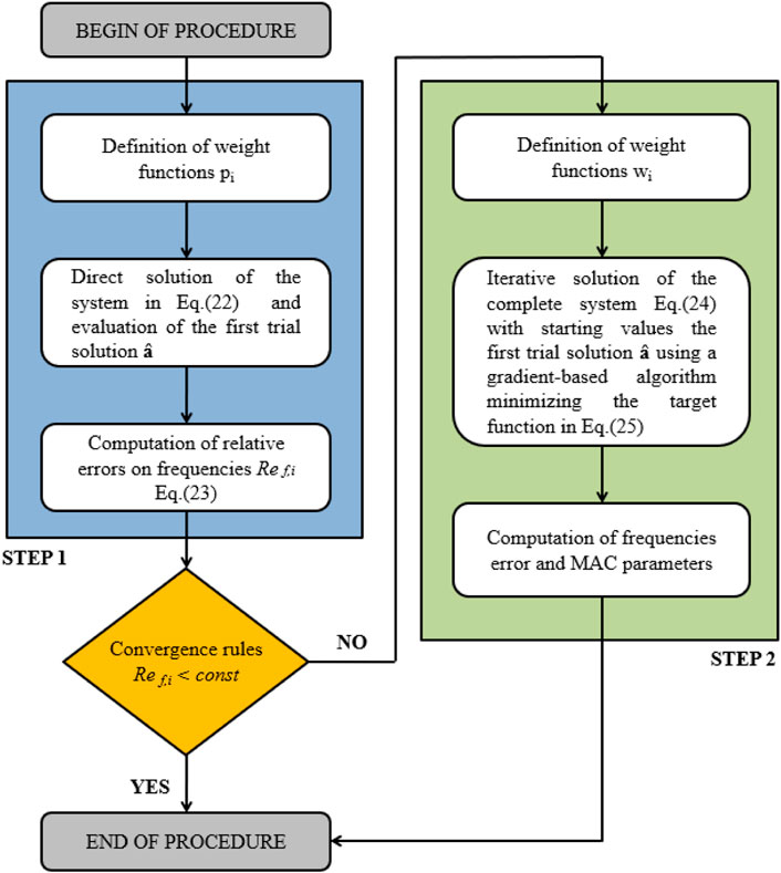
FIGURE 1. Flowchart of the two-step procedure proposed for the evaluation of unknown parameters in model updating problems.

Analogously, the mass matrix M_T of the whole system can be decomposed as:

${\mathit{M}}_T={\mathit{M}}_0+{\displaystyle \sum _{s=q+1}^N}{a}_s{\mathit{M}}_s(2)$

where: a_s (with s = q+1, q+2, …, N), are the parametric multipliers of the mass matrices ${\mathit{M}}_s\in R^{m\times m}$ and ${\mathit{M}}_0\in R^{m\times m}$ is the part of the mass matrix considered fixed (i.e., not updated) in the procedure.

2.1 First step

The standard dynamic eigenvalue problem (Clough et al., 1995) is written and a set of residuals ${\mathit{\nu }}_1,...,{\mathit{\nu }}_n$, to be minimized in a least squares problem, IS defined as:

$\left\{\begin{array}{c}{p}_1\left[{\mathit{K}}_0+{\displaystyle \sum _{s=1}^q}\left(a_s{\mathit{K}}_s\right)-{\omega }_1^2{\mathit{M}}_0-{\omega }_1^2{\displaystyle \sum _{s=q+1}^N}\left(a_s{\mathit{M}}_s\right)\right]{\mathit{\phi }}_1={\mathit{\nu }}_1\\ ⋮\\ p_i\left[{\mathit{K}}_0+{\displaystyle \sum _{s=1}^N}\left(a_s{\mathit{K}}_s\right)-{\omega }_i^2{\mathit{M}}_0-{\omega }_i^2{\displaystyle \sum _{s=q+1}^N}\left(a_s{\mathit{M}}_s\right)\right]{\mathit{\phi }}_i={\mathit{\nu }}_i\\ ⋮\\ p_n\left[{\mathit{K}}_0+{\displaystyle \sum _{s=1}^N}\left(a_s{\mathit{K}}_s\right)-{\omega }_n^2{\mathit{M}}_0-{\omega }_n^2{\displaystyle \sum _{s=q+1}^N}\left(a_s{\mathit{M}}_s\right)\right]{\mathit{\phi }}_n={\mathit{\nu }}_n\end{array}\right.(3)$

where: ω_i and ${\mathit{\phi }}_i$ are respectively the i-th experimentally identified circular frequency and mode shape; n is the number of considered modes; p_i are the weight coefficients. Each one of the n equations in Eq. 3 contains m scalar equations, where m is the degree-of-freedom number. These scalar equations are not linearly independent among them. For this reason, they constitute a redundant system. If the exact frequencies and mode shapes are introduced in Eq. 3, all the residuals are null vectors. Considering instead an experimental set of modal parameters identified from vibration records in an existing structure, typically the components of the residuals are not zero due to signal measurements noise and model errors (i.e., approximations introduced by numerical models). Therefore, the system of Eq. 3 is usually over-determined. The multiplier values $a_s$ can be calculated to obtain the best fit between experimental and numerical results.

Then, in the first step, the well-known linear least squares problem can be applied and the multiplier values are obtained by minimizing the objective function H(a_s):

$a_s=\arg \min \left(H\left(a_s\right)\right)$

with:

$H\left(a_s\right)={\displaystyle \sum _{i=1}^n}{‖{\mathit{v}}_i‖}^2(4)$

In Eq. 3, weight factors p_i have been introduced in order to drive the solution to a reliable mechanical interpretation taking into consideration the whole available experimental natural modes set (also including those having less influence in the definition of the global structural behavior). Furthermore, to improve the precision of numerical outcomes, mode shapes should be scaled to obtain residuals with the same order of magnitude among different vibrating modes. The scaling could be done, for instance, by using the mass-normalized mode shapes.

In order to achieve an explicit relation, the least squares problem is written as:

$\mathit{B}\mathit{a}=\mathit{c}(5)$

where a is the column vector of the unknown multipliers of dimensions N × 1:

$\mathit{a}={\left[a_1,...,a_s,...,a_N\right]}^T(6)$

c is a vector of dimensions n × 1:

$\mathit{c}=\left[\begin{array}{c}{p}_1\left({\omega }_1^2{\mathit{M}}_0-{\mathit{K}}_0\right){\mathit{\phi }}_1\\ ...\\ p_i\left({\omega }_i^2{\mathit{M}}_0-{\mathit{K}}_0\right){\mathit{\phi }}_i\\ ...\\ p_n\left({\omega }_n^2{\mathit{M}}_0-{\mathit{K}}_0\right){\mathit{\phi }}_n\end{array}\right](7)$

and B is the coefficient matrix of dimension n·m × N:

$\mathit{B}=\left[\mathit{Q},\mathit{R}\right](8)$

In Eq. 8 Q is an n∙m × q matrix, R is an n∙m × N-q matrix. They are respectively defined as:

$\mathit{Q}=\left[\begin{array}{ccccc}{p}_1{\mathit{K}}_1{\mathit{\phi }}_1& ...& p_1{\mathit{K}}_s{\mathit{\phi }}_1& ...& p_1{\mathit{K}}_q{\mathit{\phi }}_1\\ ...& ...& ...& ...& ...\\ p_i{\mathit{K}}_1{\mathit{\phi }}_i& ...& p_i{\mathit{K}}_s{\mathit{\phi }}_i& ...& p_i{\mathit{K}}_q{\mathit{\phi }}_i\\ ...& ...& ...& ...& ...\\ p_n{\mathit{K}}_1{\mathit{\phi }}_n& ...& p_n{\mathit{K}}_s{\mathit{\phi }}_n& ...& p_n{\mathit{K}}_q{\mathit{\phi }}_n\end{array}\right](9)$

$\mathit{R}=\left[\begin{array}{ccccc}-p_1{\omega }_1^2{\mathit{M}}_{q+1}{\mathit{\phi }}_1& ...& -p_1{\omega }_1^2{\mathit{M}}_s{\mathit{\phi }}_1& ...& -p_1{\omega }_1^2{\mathit{M}}_N{\mathit{\phi }}_1\\ ...& ...& ...& ...& ...\\ -p_i{\omega }_i^2{\mathit{M}}_{q+1}{\mathit{\phi }}_i& ...& -p_i{\omega }_i^2{\mathit{M}}_s{\mathit{\phi }}_i& ...& -p_i{\omega }_i^2{\mathit{M}}_N{\mathit{\phi }}_i\\ ...& ...& ...& ...& ...\\ -p_n{\omega }_n^2{\mathit{M}}_{q+1}{\mathit{\phi }}_n& ...& -p_n{\omega }_n^2{\mathit{M}}_s{\mathit{\phi }}_n& ...& -p_n{\omega }_n^2{\mathit{M}}_N{\mathit{\phi }}_n\end{array}\right](10)$

An estimate $\widehat{\mathit{a}}$ of the unknown multipliers a, is obtained by inverting the system in Eq. 5:

$\widehat{\mathit{a}}={\mathit{B}}^{+}\mathit{c}(11)$

in which ${\mathit{B}}^{+}$ is the pseudo-inverse of matrix B:

${\mathit{B}}^{+}={\left({\mathit{B}}^{\mathit{T}}\mathit{B}\right)}^{-\mathbf{1}}{\mathit{B}}^{\mathit{T}}(12)$

Regarding the validity of the solution of Eq. 11, the matters related to the well-posedness condition of the identification problem and the evaluation of the maximum number of identifiable parameters are discussed in Sections 2.3, 2.4.

Alternatively, the system in Eq. 3 can be conveniently reformulated in the following way:

$\stackrel{\sim }{\mathit{A}}\hspace{0.33em}\mathit{a}=\stackrel{\sim }{\mathit{b}}(13)$

where: $\stackrel{\sim }{\mathit{A}}$ is a $N\times N$ symmetric and positive-definite matrix and $\stackrel{\sim }{\mathit{b}}$ is a $N\times 1$ vector whose components are estimated by Eq. 14 and Eq. 15 respectively.

${\mathit{A}}_{s_1,s_2}=\left\{\begin{array}{cc}{\left({\stackrel{\sim }{\mathit{K}}}_{s_1}\stackrel{\sim }{\mathit{\phi }}\right)}^{\mathit{T}}\left({\stackrel{\sim }{\mathit{K}}}_{s_2}\stackrel{\sim }{\mathit{\phi }}\right)& \text{if}\hspace{0.33em}1\le s_1,s_2\le q\\ {\left({\stackrel{\sim }{\mathit{K}}}_{s_1}\stackrel{\sim }{\mathit{\phi }}\right)}^{\mathit{T}}\left({\stackrel{\sim }{\mathit{M}}}_{s_2}\stackrel{\sim }{\mathit{\phi }}\right)& \text{if}\hspace{0.33em}1\le s_1\le q\hspace{0.33em}\text{and}\hspace{0.33em}q+1\le s_2\le N\\ {\left({\stackrel{\sim }{\mathit{M}}}_{s_1}\stackrel{\sim }{\mathit{\phi }}\right)}^{\mathit{T}}\left({\stackrel{\sim }{\mathit{K}}}_{s_2}\stackrel{\sim }{\mathit{\phi }}\right)& \text{if}\hspace{0.33em}q+1\le s_1\le N\hspace{0.33em}\text{and}\hspace{0.33em}1\le s_2\le q\\ {\left({\stackrel{\sim }{\mathit{M}}}_{s_1}\stackrel{\sim }{\mathit{\phi }}\right)}^{\mathit{T}}\left({\stackrel{\sim }{\mathit{M}}}_{s_2}\stackrel{\sim }{\mathit{\phi }}\right)& \text{if}\hspace{0.33em}q+1\le s_1,s_2\le N\end{array}\right.(14)$

$b_s=\left\{\begin{array}{cc}{\left({\stackrel{\sim }{\mathit{K}}}_s\stackrel{\sim }{\mathit{\phi }}\right)}^{\mathit{T}}\stackrel{\sim }{\mathit{\psi }}& \text{if}\hspace{0.33em}1\le s\le q\\ {\left({\stackrel{\sim }{\mathit{M}}}_s\stackrel{\sim }{\mathit{\phi }}\right)}^{\mathit{T}}\stackrel{\sim }{\mathit{\psi }}& \text{if}\hspace{0.33em}q+1\le s\le N\end{array}\right.(15)$

Denoting with $\mathit{\Phi }\in R^{m\times n}$ the eigenvector matrix of the n experimentally identified vibrating modes, the vector $\stackrel{\sim }{\mathit{\phi }}$ can be defined as follows:

$\stackrel{\sim }{\mathit{\phi }}=vec\left(\mathit{\Phi }\right)(16)$

Moreover, the vector $\stackrel{\sim }{\mathit{\psi }}$ and the matrices ${\stackrel{\sim }{\mathit{K}}}_s$, ${\stackrel{\sim }{\mathit{K}}}_0$, ${\stackrel{\sim }{\mathit{M}}}_s$, ${\stackrel{\sim }{\mathit{M}}}_0$ are defined as:

$\stackrel{\sim }{\mathit{\psi }}=\stackrel{\sim }{\mathit{M}}\stackrel{\sim }{\mathit{\phi }}-{\stackrel{\sim }{\mathit{K}}}_0\stackrel{\sim }{\mathit{\phi }}(17)$

${\stackrel{\sim }{\mathit{K}}}_s=\text{diag}\left(p_i\right)\otimes {\mathit{K}}_s(18)$

${\stackrel{\sim }{\mathit{K}}}_0=\text{diag}\left(p_i\right)\otimes {\mathit{K}}_0(19)$

${\stackrel{\sim }{\mathit{M}}}_s=\text{diag}\left(-p_i{\omega }_i^2\right)\otimes {\mathit{M}}_s(20)$

${\stackrel{\sim }{\mathit{M}}}_0=\text{diag}\left(p_i{\omega }_i^2\right)\otimes {\mathit{M}}_0(21)$

The symbol “$\otimes$” indicates the Kronecker product and diag means a diagonal matrix with the i-th value equal to the argument ($p_i$ or $p_i{\omega }_i^2$). $\stackrel{\sim }{\mathit{A}}$ is symmetric and, for the uniqueness condition, it is a positive-definite matrix. More information about the derivation of Eqs 5–21 can be found in Tondi (Tondi, 2018). Finally, with the use of the new terms defined above, the assessment of the vector â, which contains the structural parameter multipliers a_s, is explicitly obtained as in the following:

$\widehat{\mathit{a}}={\stackrel{\sim }{\mathit{A}}}^{-\mathbf{1}}\stackrel{\sim }{\mathit{b}}(22)$

It is worth noting that Eqs 11, 22 directly provide the values of the unknown stiffness multipliers without the need for any iterative process. The solution of the system in Eq. 3 in common applications can provide a good fit with the experimental mode shapes, even in the case of noisy data. Nevertheless, it could assess the natural frequency values poorly.

2.2 Second step

Even though, in some applications, only the first step is needed, the second step improves the accuracy of the identified parameters in the case the natural frequencies are assessed with low precision or in general with an error higher than the required tolerance. In this study, if all the relative errors (RE) in terms of frequency values reach the prescribed tolerance, i.e.,:

$R{E}_{f,i}=\left|\frac{f_i-{\overline{f}}_i}{{\overline{f}}_i}\right|<cons{t}_i(23)$

the first step is considered satisfactory and then sufficient to reach a suitable assessment. In Eq. 23 $f_i$, and ${\overline{f}}_i$ are respectively the numerical and the experimental frequencies and const_i are the prescribed tolerance values. In the examples described in the following, const has been assumed constant for all frequencies and equal to 0.02.

If the relative errors do not satisfy Eq. 23, an improvement, i.e., the second step, is introduced in order to better fit the experimental frequency values. In the second step, a second block of equations is merged with the system in Eq. 3 as follows:

$\left\{\begin{array}{c}{p}_1\left[{\mathit{K}}_0+{\displaystyle \sum _{s=1}^N}\left(a_s{\mathit{K}}_s\right)-{\omega }_1^2{\mathit{M}}_0-{\omega }_1^2{\displaystyle \sum _{s=q+1}^N}\left(a_s{\mathit{M}}_s\right)\right]\cdot {\mathit{\phi }}_1={\mathit{\nu }}_1\\ ⋮\\ p_i\left[{\mathit{K}}_0+{\displaystyle \sum _{s=1}^N}\left(a_s{\mathit{K}}_s\right)-{\omega }_i^2{\mathit{M}}_0-{\omega }_i^2{\displaystyle \sum _{s=q+1}^N}\left(a_s{\mathit{M}}_s\right)\right]\cdot {\mathit{\phi }}_i={\mathit{\nu }}_i\\ ⋮\\ p_n\left[{\mathit{K}}_0+{\displaystyle \sum _{s=1}^N}\left(a_s{\mathit{K}}_s\right)-{\omega }_n^2{\mathit{M}}_0-{\omega }_n^2{\displaystyle \sum _{s=q+1}^N}\left(a_s{\mathit{M}}_s\right)\right]\cdot {\mathit{\phi }}_n={\mathit{\nu }}_n\\ \frac{p_1}{w_1}\mathit{det}\left[{\mathit{K}}_0+{\displaystyle \sum _{s=1}^N}\left(a_s{\mathit{K}}_s\right)-{\omega }_1^2{\mathit{M}}_0-{\omega }_1^2{\displaystyle \sum _{s=q+1}^N}\left(a_s{\mathit{M}}_s\right)\right]=r_1\\ ⋮\\ \frac{p_i}{w_i}\mathit{det}\left[{\mathit{K}}_0+{\displaystyle \sum _{s=1}^N}\left(a_s{\mathit{K}}_s\right)-{\omega }_i^2{\mathit{M}}_0-{\omega }_i^2{\displaystyle \sum _{s=q+1}^N}\left(a_s{\mathit{M}}_s\right)\right]=r_i\\ ⋮\\ \frac{p_n}{w_n}\mathit{det}\left[{\mathit{K}}_0+{\displaystyle \sum _{\mathit{s}=\mathbf{1}}^N}\left({\mathit{a}}_{\mathit{s}}{\mathit{K}}_s\right)-{\omega }_n^2{\mathit{M}}_0-{\omega }_n^2{\displaystyle \sum _{s=q+1}^{\mathit{N}}}\left(a_s{\mathit{M}}_s\right)\right]=r_n\end{array}\right.(24)$

The second equation block explicitly involves the null value of the determinants only if the exact eigenvalues are introduced. As a result, the system of Eq. 24 is even more redundant than the system of Eq. 3 and, consequently, mathematically more constrained. Due to the non-linearity introduced by the second block, it is not possible to obtain directly (i.e., explicitly) the improved solution, and then the second step introduces an iterative process.

It is worth noting that residuals from the eigenvalue equations block (i.e., the second block in Eq. 24) typically have values greater than those obtained from the eigenvector equations block (i.e., the first block in Eq. 24). As a consequence, a set of weight parameters $w_i$ (with i = 1, 2, …, n) is introduced in Eq. 24 to ensure that the first and second equation blocks provide residuals with analogous order of magnitude. They do not have a physical means, but their introduction allows to achieve the solution at a higher rate of speed.

In the second step, the objective function to minimize is thus defined as the sum between the second-norm of the residuals vector ${\mathit{\nu }}_i$ and the sum of squared residuals r_i:

$H\left(a_s\right)={\displaystyle \sum _{i=1}^n}\left({‖{\mathit{\nu }}_i‖}^2+{r_i}^2\right)(25)$

The solution of Eq. 25 is obtained in the present proposal by using a standard gradient-based optimization algorithm (Coleman and Li, 1996; Conn et al., 2000), for which the solution $\widehat{\mathit{a}}$ of Eq. 22, i.e., the solution obtained from the first step, is assumed as the initial value for the second step. The (iterative) solution of the complete system leads to an improvement in the assessment of the frequency values without affecting the accuracy of the estimated mode shapes. The two-step procedure described here has been introduced as a routine in the MATLAB (MathWorks, 2023) environment following the flowchart shown in Figure 1.

2.3 Maximum (theoretical) number of identifiable parameters

Starting from the dynamic eigenvalue/eigenvector problem, it is possible to prove that the maximum theoretical number (N_max) of identifiable parameters is:

$N_{\mathit{max}}=n\cdot \left(m+1\right)-{\displaystyle \sum _{i=1}^n}i(26)$

where n is the number of considered vibrating modes and m is the number of degrees of freedom. The proof and demonstration of Eq. 26 is reported in Appendix. This value provides important information because it represents the upper bound of the practical maximum number of unknowns identifiable with the available dataset.

2.4 Uniqueness of the solution

The uniqueness of the solution for the linear system in Eq. 13 is ensured if:

$\det \left(\stackrel{\sim }{\mathit{A}}\right)\ne 0(27)$

Reasoning on the contrary, for the sake of simplicity, the uniqueness of the solution is not guaranteed in the case that the determinant has a null value. After some trivial mathematical operations, the null value of the determinant can be achieved if there exists a set of parameters a = $\left({\alpha }_1,{\alpha }_2,\dots ,{\alpha }_N\right)∊R^N$ whereby:

${\alpha }_1{\stackrel{\sim }{\mathbf{K}}}_1\stackrel{\sim }{\mathbf{\phi }}+{\alpha }_2{\stackrel{\sim }{\mathbf{K}}}_2\stackrel{\sim }{\mathbf{\phi }}+\dots +{\alpha }_q{\stackrel{\sim }{\mathbf{K}}}_{\mathrm{q}}\stackrel{\sim }{\mathbf{\phi }}+{\alpha }_{q+1}{\stackrel{\sim }{\mathbf{M}}}_{\mathrm{q}+1}\stackrel{\sim }{\mathbf{\phi }}+\dots +{\alpha }_N{\stackrel{\sim }{\mathbf{M}}}_{\mathrm{N}}\stackrel{\sim }{\mathbf{\phi }}=\mathbf{0}(28)$

Equation 27 is therefore satisfied if and only if the vectors ${\stackrel{\sim }{\mathbf{K}}}_1\stackrel{\sim }{\mathbf{\phi }},{\stackrel{\sim }{\mathbf{K}}}_2\stackrel{\sim }{\mathbf{\phi }},\dots ,{\stackrel{\sim }{\mathbf{K}}}_{\mathrm{q}}\stackrel{\sim }{\mathbf{\phi }},{\stackrel{\sim }{\mathbf{M}}}_{\mathrm{q}+1}\stackrel{\sim }{\mathbf{\phi }},\dots ,{\stackrel{\sim }{\mathbf{M}}}_{\mathrm{N}}\stackrel{\sim }{\mathbf{\phi }}$ are linearly independent and if:

${\stackrel{\sim }{\mathbf{K}}}_{\mathrm{s}}\stackrel{\sim }{\mathbf{\phi }}\ne \mathbf{0}(29)$

for s = 1, 2, …, q, associated with:

${\stackrel{\sim }{\mathbf{M}}}_{\mathrm{t}}\stackrel{\sim }{\mathbf{\phi }}\ne \mathbf{0}(30)$

for t = q+1, q+2, …, N. These conditions are N + 1 in total. The reader could refer to Tondi (Tondi, 2018) for a detailed mathematical demonstration.

2.5 Definiteness of the Hessian matrix

Computing the second derivatives of the objective function H(a_s) (Eq. 4) with respect to the multipliers a_s, the Hessian matrix $\stackrel{\sim }{\mathbf{H}}$ of the problem can be computed. After some mathematical calculations, not reported here for the sake of brevity, the Hessian matrix can be expressed in the following way:

$\stackrel{\sim }{\mathbf{H}}=2\stackrel{\sim }{\mathbf{A}}(31)$

Exploiting the definition of definiteness itself, the following relation can be found:

$\left[x_1{x}_2\cdots x_n\right]\bullet \stackrel{\sim }{\mathit{H}}\bullet \left[\begin{array}{c}\begin{array}{c}{x}_1\\ x_2\end{array}\\ ⋮\\ x_n\end{array}\right]=2\bullet {‖x_1{\stackrel{\sim }{\mathbf{K}}}_1\stackrel{\sim }{\mathbf{\phi }}+x_2{\stackrel{\sim }{\mathbf{K}}}_2\stackrel{\sim }{\mathbf{\phi }}+\dots +x_n{\stackrel{\sim }{\mathbf{M}}}_{\mathrm{N}}\stackrel{\sim }{\mathit{\phi }}‖}^2\ge 0(32)$

$\forall x_1,x_2,\cdots ,x_N\in \mathfrak{R}$

Therefore, the Hessian matrix $\stackrel{\sim }{\mathbf{H}}$ as the coefficient matrix $\stackrel{\sim }{\mathbf{A}}$ are semi-positive definite. Since $\stackrel{\sim }{\mathbf{A}}$ is a semi-positive definite matrix, it has eigenvalues greater than, or at least equal to, zero. Therefore, it is possible to write:

$\det \left(\stackrel{\sim }{\mathbf{A}}\right)\ge \mathbf{0}(33)$

which is a generalization of the Cauchy-Schwarz inequality. Then, a unique stationary point associated with a positive DEFINITE Hessian matrix represents a global minimum point for the target function (Tondi, 2018).

3 Uncertainty assessment

Model updating problems are inverse problems based on the minimization of an objective function. In real case applications, due to the presence of both measurement and modeling errors, the unknown parameters are unavoidably affected by uncertainty. Then, the assessment of the unknown parameter uncertainty allows to establish the robustness of the decision-making process usually based on the updated model. If the uncertainties C_e of the modal characteristics, i.e., natural frequencies and mode shapes, are known [see for instance the procedure proposed by Reynders et al. (2008)] the procedure described in this subsection allows us to directly estimate the standard deviations of the structural parameters. The problem has been approached by using the error propagation theory (Taylor, 1997). Therefore, the covariance matrix C_a of the obtained structural multipliers a is evaluated by means of the equation:

${\mathbf{C}}_a={\mathbf{J}}_a{\mathbf{C}}_e{\mathbf{J}}_a^{\mathit{T}}(34)$

where J_a is the Jacobian matrix collecting the partial derivatives of the multipliers a₁–a_N, with respect to the natural frequencies ω₁–ω_n, and the mode shapes components φ₁₁–φ_mn:

${\mathbf{J}}_a=\left[\begin{array}{cccccccccc}\frac{\partial a_1}{\partial {\phi }_{11}}& \cdots & \frac{\partial a_1}{\partial {\phi }_{ji}}& \cdots & \frac{\partial a_1}{\partial {\phi }_{mn}}& \frac{\partial a_1}{\partial {\omega }_1^2}& \cdots & \frac{\partial a_1}{\partial {\omega }_i^2}& \cdots & \frac{\partial a_1}{\partial {\omega }_n^2}\\ ⋮& & ⋮& & ⋮& ⋮& & ⋮& & ⋮\\ \frac{\partial a_s}{\partial {\phi }_{11}},& \cdots & \frac{\partial a_s}{\partial {\phi }_{ji}},& \cdots & \frac{\partial a_s}{\partial {\phi }_{mn}},& \frac{\partial a_s}{\partial {\omega }_1^2}& \cdots & \frac{\partial a_s}{\partial {\omega }_i^2}& \cdots & \frac{\partial a_s}{\partial {\omega }_n^2}\\ ⋮& & ⋮& & ⋮& ⋮& & ⋮& & ⋮\\ \frac{\partial a_N}{\partial {\phi }_{11}},& \cdots & \frac{\partial a_N}{\partial {\phi }_{ji}},& \cdots & \frac{\partial a_N}{\partial {\phi }_{mn}},& \frac{\partial a_N}{\partial {\omega }_1^2}& \cdots & \frac{\partial a_N}{\partial {\omega }_i^2}& \cdots & \frac{\partial a_N}{\partial {\omega }_n^2}\end{array}\right](35)$

and C_e is the covariance matrix of experimental circular frequency squares ${\omega }_i^2$ and mode shape components ${\phi }_{ji}$:

${\mathbf{C}}_{\mathit{e}}=\left[\begin{array}{cccccccccc}{\mathrm{\sigma }}_{{\mathrm{\phi }}_{11}}^2& \cdots & cov\left({\mathrm{\phi }}_{11};{\mathrm{\phi }}_{\text{ji}}\right)& \cdots & cov\left({\mathrm{\phi }}_{11};{\mathrm{\phi }}_{mn}\right)& cov\left({\mathrm{\phi }}_{11};{\mathrm{\omega }}_1^2\right)& \cdots & cov\left({\mathrm{\phi }}_{11};{\mathrm{\omega }}_i^2\right)& \cdots & cov\left({\mathrm{\phi }}_{11};{\mathrm{\omega }}_n^2\right)\\ ⋮& ⋮& ⋮& ⋮& ⋮& ⋮& ⋮& ⋮& ⋮& ⋮\\ cov\left({\mathrm{\phi }}_{ji};{\mathrm{\phi }}_{11}\right)& \cdots & {\mathrm{\sigma }}_{{\mathrm{\phi }}_{ji}}^2& \cdots & cov\left({\mathrm{\phi }}_{ji};{\mathrm{\phi }}_{mn}\right)& cov\left({\mathrm{\phi }}_{ji};{\mathrm{\omega }}_1^2\right)& \cdots & cov\left({\mathrm{\phi }}_{ji};{\mathrm{\omega }}_i^2\right)& \cdots & cov\left({\mathrm{\phi }}_{ji};{\mathrm{\omega }}_n^2\right)\\ ⋮& ⋮& ⋮& \ddots & ⋮& ⋮& ⋮& ⋮& ⋮& ⋮\\ cov\left({\mathrm{\phi }}_{mn};{\mathrm{\phi }}_{11}\right)& \cdots & cov\left({\mathrm{\phi }}_{mn};{\mathrm{\phi }}_{ji}\right)& \cdots & {\mathrm{\sigma }}_{{\mathrm{\phi }}_{mn}}^2& cov\left({\mathrm{\phi }}_{mn};{\mathrm{\omega }}_1^2\right)& \cdots & cov\left({\mathrm{\phi }}_{mn};{\mathrm{\omega }}_i^2\right)& \cdots & cov\left({\mathrm{\phi }}_{mn};{\mathrm{\omega }}_n^2\right)\\ cov\left({\mathrm{\omega }}_1^2;{\mathrm{\phi }}_{11}\right)& \cdots & cov\left({\mathrm{\omega }}_1^2;{\mathrm{\phi }}_{ji}\right)& \cdots & cov\left({\mathrm{\omega }}_1^2;{\mathrm{\phi }}_{mn}\right)& {\mathrm{\sigma }}_{{\mathrm{\omega }}_1^2}^2& \cdots & cov\left({\mathrm{\omega }}_1^2;{\mathrm{\omega }}_i^2\right)& \cdots & cov\left({\mathrm{\omega }}_1^2;{\mathrm{\omega }}_n^2\right)\\ ⋮& ⋮& ⋮& ⋮& ⋮& ⋮& \ddots & ⋮& ⋮& ⋮\\ cov\left({\mathrm{\omega }}_i^2;{\mathrm{\phi }}_{11}\right)& \cdots & cov\left({\mathrm{\omega }}_i^2;{\mathrm{\phi }}_{ji}\right)& \cdots & cov\left({\mathrm{\omega }}_i^2;{\mathrm{\phi }}_{mn}\right)& cov\left({\mathrm{\omega }}_i^2;{\mathrm{\omega }}_1^2\right)& \cdots & {\mathrm{\sigma }}_{{\mathrm{\omega }}_{\mathrm{i}}^2}^2& \cdots & cov\left({\mathrm{\omega }}_i^2;{\mathrm{\omega }}_n^2\right)\\ ⋮& ⋮& ⋮& ⋮& ⋮& ⋮& ⋮& ⋮& \ddots & ⋮\\ cov\left({\mathrm{\omega }}_n^2;{\mathrm{\phi }}_{11}\right)& \cdots & cov\left({\mathrm{\omega }}_n^2;{\mathrm{\phi }}_{ji}\right)& \cdots & cov\left({\mathrm{\omega }}_n^2;{\mathrm{\phi }}_{mn}\right)& cov\left({\mathrm{\omega }}_n^2;{\mathrm{\omega }}_1^2\right)& \cdots & cov\left({\mathrm{\omega }}_n^2;{\mathrm{\omega }}_i^2\right)& \cdots & {\mathrm{\sigma }}_{{\mathrm{\omega }}_{\mathrm{n}}^2}^2\end{array}\right](36)$

Then, the standard deviation σ_a,s of each unknown parameter a_s can be computed using the following expression:

${\sigma }_{a,s}\cong \sqrt{\nabla {{\mathit{a}}_s}^T{\mathit{C}}_e\nabla {\mathit{a}}_s}(37)$

where s = 1, 2, …, N and:

$\nabla {\mathit{a}}_{\mathit{s}}={\left[\begin{array}{cccccc}\frac{\partial a_s}{\partial {\phi }_{11}},& ...,& \frac{\partial a_s}{\partial {\phi }_{mn}},& \frac{\partial a_s}{\partial {\omega }_1^2},& ...,& \frac{\partial a_s}{\partial {\omega }_n^2}\end{array}\right]}^T(38)$

The Jacobian matrix J_a has to be computed before calculating the covariance matrix C_a. The partial derivatives of the unknown parameters with respect to the experimental outcomes are denoted as:

$\frac{\partial \mathit{a}}{\partial {\phi }_{ji}}={\left[\begin{array}{cccccc}\frac{\partial a_1}{\partial {\phi }_{ji}},& ...,& \frac{\partial a_q}{\partial {\phi }_{ji}},& \frac{\partial a_{q+1}}{\partial {\phi }_{ji}},& ...,& \frac{\partial a_N}{\partial {\phi }_{ji}}\end{array}\right]}^T(39)$

$\frac{\partial \mathit{a}}{\partial {\omega }_i^2}={\left[\begin{array}{cccccc}\frac{\partial a_1}{\partial {\omega }_i^2},& ...,& \frac{\partial a_q}{\partial {\omega }_i^2},& \frac{\partial a_{q+1}}{\partial {\omega }_i^2},& ...,& \frac{\partial a_N}{\partial {\omega }_i^2}\end{array}\right]}^T(40)$

and after some mathematical calculations, it is possible to express the partial derivatives as:

$\stackrel{\sim }{\mathit{A}}\cdot \frac{\partial \mathit{a}}{\partial {\phi }_{ji}}={\stackrel{\sim }{\mathit{l}}}_{ji}(41)$

$\stackrel{\sim }{\mathit{A}}\cdot \frac{\partial \mathit{a}}{\partial {\omega }_i^2}={\stackrel{\sim }{\mathit{r}}}_i(42)$

where: i = 1, 2, …, n and j = 1, 2, …, m. Moreover, we can define the vectors:

${\stackrel{\sim }{\mathit{l}}}_{ji}={\left[\begin{array}{cccccc}{\stackrel{\sim }{l}}_{1,ji},& ...& {\stackrel{\sim }{l}}_{q,ji},& {\stackrel{\sim }{l}}_{q+1,ji},& ...& {\stackrel{\sim }{l}}_{N,ji}\end{array}\right]}^T(\mathrm{43a})$

and:

${\stackrel{\sim }{\mathit{r}}}_i={\left[\begin{array}{cccccc}{\stackrel{\sim }{r}}_{1,i},& ...& {\stackrel{\sim }{r}}_{q,i},& {\stackrel{\sim }{r}}_{q+1,i},& ...& {\stackrel{\sim }{r}}_{N,i}\end{array}\right]}^T(\mathrm{43b})$

both with dimensions N×1 and whose components are defined in the following way:

$\begin{array}{ll}\hfill {\stackrel{\sim }{l}}_{s,ji}& =-{\sum }_{k=1}^q{a}_k\left[{\left({\stackrel{\sim }{\mathit{K}}}_s^{\left(i-1\right)m+j}\right)}^T\left({\stackrel{\sim }{\mathit{K}}}_k\stackrel{\sim }{\mathit{\phi }}\right)+{\left({\stackrel{\sim }{\mathit{K}}}_k^{\left(i-1\right)m+j}\right)}^T\left({\stackrel{\sim }{\mathit{K}}}_s\stackrel{\sim }{\mathit{\phi }}\right)\right]\hfill \\ \hfill & -{\sum }_{k=q+1}^N{a}_k\left[{\left({\stackrel{\sim }{\mathit{K}}}_s^{\left(i-1\right)m+j}\right)}^T\left({\stackrel{\sim }{\mathit{M}}}_k\stackrel{\sim }{\mathit{\phi }}\right)+{\left({\stackrel{\sim }{\mathit{M}}}_k^{\left(i-1\right)m+j}\right)}^T\left({\stackrel{\sim }{\mathit{K}}}_s\stackrel{\sim }{\mathit{\phi }}\right)\right]\hfill \\ \hfill & +{\left({\stackrel{\sim }{\mathit{K}}}_s^{\left(i-1\right)m+j}\right)}^T\stackrel{\sim }{\mathit{\psi }}+{\left({\stackrel{\sim }{\mathit{M}}}_0^{\left(i-1\right)m+j}-{\stackrel{\sim }{\mathit{K}}}_0^{\left(i-1\right)m+j}\right)}^T\left({\stackrel{\sim }{\mathit{K}}}_s\stackrel{\sim }{\mathit{\phi }}\right)\hfill \end{array}(44)$

${\stackrel{\sim }{r}}_{s,i}=-{\displaystyle \sum _{k=q+1}^N}{a}_k{\left({\stackrel{\sim }{\mathit{K}}}_s\stackrel{\sim }{\mathit{\phi }}\right)}^T\left({\stackrel{\sim }{\mathit{M}}}_{k,i}\stackrel{\sim }{\mathit{\phi }}\right)+{\left({\stackrel{\sim }{\mathit{K}}}_s\stackrel{\sim }{\mathit{\phi }}\right)}^T\left({\stackrel{\sim }{\mathit{M}}}_{0,i}\stackrel{\sim }{\mathit{\phi }}\right)(45)$

for s = 1, 2, …, q and:

$\begin{array}{ll}\hfill {\stackrel{\sim }{l}}_{s,ji}& =-{\displaystyle \sum _{k=1}^q}{a}_k\left[{\left({\stackrel{\sim }{\mathit{M}}}_s^{\left(i-1\right)m+j}\right)}^T\left({\stackrel{\sim }{\mathit{K}}}_k\stackrel{\sim }{\mathit{\phi }}\right)+{\left({\stackrel{\sim }{\mathit{K}}}_k^{\left(i-1\right)m+j}\right)}^T\left({\stackrel{\sim }{\mathit{M}}}_s\stackrel{\sim }{\mathit{\phi }}\right)\right]\hfill \\ \hfill & -{\displaystyle \sum _{k=q+1}^N}{a}_k\left[{\left({\stackrel{\sim }{\mathit{M}}}_s^{\left(i-1\right)m+j}\right)}^T\left({\stackrel{\sim }{\mathit{M}}}_k\stackrel{\sim }{\mathit{\phi }}\right)+{\left({\stackrel{\sim }{\mathit{M}}}_k^{\left(i-1\right)m+j}\right)}^T\left({\stackrel{\sim }{\mathit{M}}}_s\stackrel{\sim }{\mathit{\phi }}\right)\right]\hfill \\ \hfill & +{\left({\stackrel{\sim }{\mathit{M}}}_s^{\left(i-1\right)m+j}\right)}^T\stackrel{\sim }{\mathit{\psi }}+{\left({\stackrel{\sim }{\mathit{M}}}_0^{\left(i-1\right)m+j}-{\stackrel{\sim }{\mathit{K}}}_0^{\left(i-1\right)m+j}\right)}^T\left({\stackrel{\sim }{\mathit{M}}}_s\stackrel{\sim }{\mathit{\phi }}\right)\hfill \end{array}(46)$

${\stackrel{\sim }{r}}_{s,i}=-{\displaystyle \sum _{k=1}^N}{a}_k{\left({\stackrel{\sim }{\mathit{K}}}_k\stackrel{\sim }{\mathit{\phi }}\right)}^T\left({\stackrel{\sim }{\mathit{M}}}_{s,i}\stackrel{\sim }{\mathit{\phi }}\right)-{\displaystyle \sum _{k=q+1}^N}{a}_k\left[{\left({\stackrel{\sim }{\mathit{M}}}_s\stackrel{\sim }{\mathit{\phi }}\right)}^T\left({\stackrel{\sim }{\mathit{M}}}_{k,i}\stackrel{\sim }{\mathit{\phi }}\right)+{\left({\stackrel{\sim }{\mathit{M}}}_k\stackrel{\sim }{\mathit{\phi }}\right)}^T\left({\stackrel{\sim }{\mathit{M}}}_{s,i}\stackrel{\sim }{\mathit{\phi }}\right)\right]+{\left({\stackrel{\sim }{\mathit{M}}}_{s,i}\stackrel{\sim }{\mathit{\phi }}\right)}^T\stackrel{\sim }{\mathit{\psi }}+{\left({\stackrel{\sim }{\mathit{M}}}_s\stackrel{\sim }{\mathit{\phi }}\right)}^T\left({\stackrel{\sim }{\mathit{M}}}_{0,i}\stackrel{\sim }{\mathit{\phi }}\right)(47)$

for s = q+1, q+2, …, N.

The superscript (i–1)m + j indicates the column of the matrix to be selected. Furthermore, ${\stackrel{\sim }{\mathit{M}}}_{s,i}$ and ${\stackrel{\sim }{\mathit{M}}}_{0,i}$ are block diagonal matrices defined as:

${\stackrel{\sim }{\mathit{M}}}_{s,i}=\left[\begin{array}{cccccc}\mathbf{0}& \mathbf{0}& \cdots & \mathbf{0}& \cdots & \mathbf{0}\\ \mathbf{0}& \mathbf{0}& \cdots & \mathbf{0}& \cdots & \mathbf{0}\\ ⋮& ⋮& \ddots & ⋮& \cdots & ⋮\\ \mathbf{0}& \mathbf{0}& \cdots & -p_i{\mathit{M}}_s& \cdots & \mathbf{0}\\ ⋮& ⋮& \cdots & ⋮& \ddots & ⋮\\ \mathbf{0}& \mathbf{0}& \cdots & \mathbf{0}& \cdots & \mathbf{0}\end{array}\right](48)$

${\stackrel{\sim }{\mathit{M}}}_{0,i}=\left[\begin{array}{cccccc}\mathbf{0}& \mathbf{0}& \cdots & \mathbf{0}& \cdots & \mathbf{0}\\ \mathbf{0}& \mathbf{0}& \cdots & \mathbf{0}& \cdots & \mathbf{0}\\ ⋮& ⋮& \ddots & ⋮& \cdots & ⋮\\ \mathbf{0}& \mathbf{0}& \cdots & p_i{\mathit{M}}_0& \cdots & \mathbf{0}\\ ⋮& ⋮& \cdots & ⋮& \ddots & ⋮\\ \mathbf{0}& \mathbf{0}& \cdots & \mathbf{0}& \cdots & \mathbf{0}\end{array}\right](49)$

Finally, the partial derivatives are achieved starting from Eqs 41, 42 by inverting $\stackrel{\sim }{\mathit{A}}$, so obtaining:

$\frac{\partial \mathit{a}}{\partial {\phi }_{ji}}={\stackrel{\sim }{\mathit{A}}}^{-1}\cdot {\stackrel{\sim }{\mathit{l}}}_{ji}(50)$

$\frac{\partial \mathit{a}}{\partial {\omega }_i^2}={\stackrel{\sim }{\mathit{A}}}^{-1}\cdot {\stackrel{\sim }{\mathit{r}}}_i(51)$

The diagonal terms of the C_a matrix represent the assessment of the variance of each unknown parameter.

The assessment of the unknown parameter uncertainty described in this subsection can be applied using both the first estimate of the unknown parameters (provided by the first step of the proposed procedure) or the refined solution (available after the application of the second step). In the example of the following section, the uncertainty evaluation is conducted on the final values of the identified parameters.

4 Numerical applications to test-bed case studies

The procedure proposed in this article has been tested by performing the assessment of the stiffness values of the 2D and 3D frames selected as test-bed case studies. It is worth noting that the selected case studies are particularly simple because the authors aimed at selecting case studies where the exact solutions are known, the mathematical processes are perfectly controllable and the uncertainties of the selected parameters can be compared with those coming from a Monte Carlo simulation. In Section 5, an application to a full-scale real building (i.e., more complex and affected by both modeling and measurement errors) will be reported.

4.1 Case study 1: 2D three-story frame

4.1.1 Evaluation of multipliers in the case of exact input data

The first test-bed case study is a 2D shear-type three-story frame with three degrees of freedom (DOFs) and with two mechanical parameters to estimate. The first and the second parameters to be identified are the stiffness of the columns of the first two stories and the stiffness of the columns of the third story respectively (see Figure 2). Only the first natural frequency and the associated mode shape are assumed as input in the procedure.

FIGURE 2

FIGURE 2. Case study 1: 2D frame with indication of the two unknown parameters a₁–a₂.

The numerical example is then performed by introducing the following three stiffness matrices:

${\mathit{K}}_0=\left[\begin{array}{ccc}2& -1& 0\\ -1& 2& -1\\ 0& -1& 1\end{array}\right];{\mathit{K}}_1=\left[\begin{array}{ccc}2& -1& 0\\ -1& 1& 0\\ 0& 0& 0\end{array}\right];{\mathit{K}}_2=\left[\begin{array}{ccc}0& 0& 0\\ 0& 1& -1\\ 0& -1& 1\end{array}\right]$

The mass matrix M0 is assumed known and the same value of mass M = 0.02 for each floor is considered, so obtaining:

${\mathit{M}}_0=\left[\begin{array}{ccc}0.02& 0& 0\\ 0& 0.02& 0\\ 0& 0& 0.02\end{array}\right]$

The reference (exact) values for the parameters in order to compute the first circular frequency and the corresponding mode shape are:

$a_{1,ref}=25,a_{2,ref}=15$

The reference circular frequency and mode shape are respectively:

${\omega }_{1,ref}=15.50\hspace{0.33em}\text{rad}/\mathbf{s}$

${\mathit{\phi }}_{1,ref}=\left[\begin{array}{c}2.130\\ 3.865\\ 5.525\end{array}\right]$

Now, it is supposed that multipliers a₁ and a₂ are unknown and the procedure described in Section 2 is applied to obtain their values. The comparison between the obtained values and the reference ones is then performed. First, the matrices ${\stackrel{\sim }{\mathit{K}}}_s$, ${\stackrel{\sim }{\mathit{K}}}_0$, ${\stackrel{\sim }{\mathit{M}}}_s$, ${\stackrel{\sim }{\mathit{M}}}_0$ and the vector $\stackrel{\sim }{\mathit{\phi }}$ are computed. In this particular case, with only one available mode, they are:

$\stackrel{\sim }{\mathit{\phi }}={\mathit{\phi }}_{1,ref};{\stackrel{\sim }{\mathit{K}}}_s={\mathit{K}}_s;{\stackrel{\sim }{\mathit{K}}}_0={\mathit{K}}_0;{\stackrel{\sim }{\mathit{M}}}_s=-{\omega }_{1,ref}^2{\mathit{M}}_s;{\stackrel{\sim }{\mathit{M}}}_0={\omega }_{1,ref}^2{\mathit{M}}_0$

Then, the vector $\stackrel{\sim }{\mathit{\psi }}$ is also evaluated:

$\stackrel{\sim }{\mathit{\psi }}=\stackrel{\sim }{\mathit{M}}\stackrel{\sim }{\mathit{\phi }}-{\stackrel{\sim }{\mathit{K}}}_0\stackrel{\sim }{\mathit{\phi }}={\omega }_1^2{\mathit{M}}_0{\mathit{\phi }}_{1,ref}-{\mathit{K}}_0{\mathit{\phi }}_{1,ref}=\left[\begin{array}{c}9.841\\ 18.50\\ 24.89\end{array}\right]$

The matrix $\stackrel{\sim }{\mathit{A}}$ and the vector $\stackrel{\sim }{\mathit{b}}$ are then computed according to Eqs 14, 15:

$\stackrel{\sim }{\mathit{A}}=\left[\begin{array}{cc}{\left({\mathit{K}}_1{\mathit{\phi }}_{1,ref}\right)}^T\left({\mathit{K}}_1{\mathit{\phi }}_{1,ref}\right)& {\left({\mathit{K}}_1{\mathit{\phi }}_{1,ref}\right)}^T\left({\mathit{K}}_2{\mathit{\phi }}_{1,ref}\right)\\ {\left({\mathit{K}}_2{\mathit{\phi }}_{1,ref}\right)}^T\left({\mathit{K}}_1{\mathit{\phi }}_{1,ref}\right)& {\left({\mathit{K}}_2{\mathit{\phi }}_{1,ref}\right)}^T\left({\mathit{K}}_2{\mathit{\phi }}_{1,ref}\right)\end{array}\right]=\left[\begin{array}{cc}3.168& -2.881\\ -2.881& 5.509\end{array}\right]$

$\stackrel{\sim }{\mathit{b}}=\left[\begin{array}{c}{\left({\mathit{K}}_1{\mathit{\phi }}_{1,ref}\right)}^T\mathit{\psi }\\ {\left({\mathit{K}}_2{\mathit{\phi }}_{1,ref}\right)}^T\mathit{\psi }\end{array}\right]=\left[\begin{array}{c}35.99\\ 10.61\end{array}\right]$

Finally, the unknown structural parameter multipliers can be obtained by means of Eq. 22:

$\widehat{\mathit{a}}={\stackrel{\sim }{\mathit{A}}}^{-1}\stackrel{\sim }{\mathit{b}}=\left[\begin{array}{c}25.00\\ 15.00\end{array}\right]$

By the comparison between values obtained by using the present procedure and reference values, it is possible to observe a perfect agreement between the two pairs of values. In the absence of errors (modeling errors, measurement errors, truncating errors, etc.), the first step of the procedure is sufficient to reach the reference exact value.

4.1.2 Evaluation of multipliers in the case of noisy input data

To evaluate the effects of noisy data on the procedure, the frame story stiffnesses have been identified starting from the so-called pseudo-experimental input data. The pseudo-experimental data are obtained by adding some statistical scattering to the “exact” values of the input data. In particular, they are obtained by multiplying the exact values of frequencies and mode shape components by uncorrelated coefficients extracted from a normal probability distribution with mean value equal to 1.0 and coefficient of variation (CoV) equal to 5%. Therefore, the new pseudo-experimental (identified in the following with the subscript “PS”) input data used for the calibration of the story stiffnesses are:

${\omega }_{1,ref,PS}=15.29\hspace{0.33em}rad/s$

${\mathit{\phi }}_{1,ref,PS}=\left[\begin{array}{c}2.183\\ 3.686\\ 5.626\end{array}\right]$

The procedure shown in Section 4.1.1 allows us to find the value of the multipliers:

$\widehat{\mathit{a}}=\left[\begin{array}{c}23.91\\ 10.98\end{array}\right]$

The parameters a₁ and a₂ are then introduced in the dynamic eigenvalue/eigenvector problem and the modal parameters are then estimated. The assessment of the circular frequency ${\widehat{\omega }}_1$ and the mode shape components are:

${\widehat{\omega }}_1=14.79\hspace{0.33em}rad/s$

${\widehat{\mathit{\phi }}}_1=\left[\begin{array}{c}1.994\\ 3.637\\ 5.727\end{array}\right]$

The first natural frequency result was about 3.3% lower than the reference value ${\omega }_{1,ref,PS}$ and so, according to the criterion reported in Eq. 23, the second step of the procedure must be performed. A standard gradient-based optimization algorithm is used and, after three iterations, the new multiplier vector has been obtained. It results in:

$\widehat{\mathit{a}}=\left[\begin{array}{c}25.70\\ 11.81\end{array}\right]$

The improved frequency value and mode shape components respectively are:

${\widehat{\omega }}_1=15.30\hspace{0.33em}rad/s$

${\widehat{\mathit{\phi }}}_1=\left[\begin{array}{c}1.999\\ 3.646\\ 5.719\end{array}\right]$

The final first natural frequency value, after the two steps, is practically equal to the reference value (i.e. 15.29 rad/s). This simple example shows that, in practical problems faced with input data affected by experimental errors, the second step is fundamental to reach a high level of accuracy for the frequency value.

4.1.3 Uncertainty assessment

In this subsection, the standard deviation of the unknown parameters, i.e., the structural multipliers, are computed following the procedure described in Section 3. A CoV equal to 5% was assumed for the frequency $f_1$ and for the mode shape components. Then, the variances of the four modal parameters are:

${\sigma }_{{\varphi }_{11}}^2=0.0113,{\sigma }_{{\varphi }_{21}}^2=0.0374,{\sigma }_{{\varphi }_{31}}^2=0.0763,{\sigma }_{{\omega }_1^2}^2=578{\text{rad}}^2/{\mathrm{s}}^2$

Firstly, the partial derivatives with respect to ${\phi }_{11}$, ${\phi }_{21}$, ${\phi }_{31}$ and ${\omega }_1^2$ are computed.

• Partial derivatives with respect to ${\varphi }_{11}$:

$\stackrel{\sim }{\mathit{A}}\left[\begin{array}{c}\frac{\partial a_1}{\partial {\phi }_{11}}\\ \frac{\partial a_2}{\partial {\phi }_{11}}\end{array}\right]=\left[\begin{array}{c}{\stackrel{\sim }{l}}_{\mathrm{1,11}}\\ {\stackrel{\sim }{l}}_{\mathrm{2,11}}\end{array}\right]$

with:

${\stackrel{\sim }{l}}_{\mathrm{1,11}}=-2a_1{\left({\mathit{K}}_1^1\right)}^T\left({\mathit{K}}_1\mathit{\varphi }\right)-a_2{\left({\mathit{K}}_1^1\right)}^T\left({\mathit{K}}_2\mathit{\varphi }\right)-a_2{\left({\mathit{K}}_2^1\right)}^T\left({\mathit{K}}_1\mathit{\varphi }\right)+{\left({\omega }_1^2{\mathit{M}}_0^1-{\mathit{K}}_0^1\right)}^T\left({\mathit{K}}_1\mathit{\varphi }\right)+{\mathit{\psi }}^T\left({\mathit{K}}_1^1\right)$

${\stackrel{\sim }{l}}_{\mathrm{2,11}}=-2a_2{\left({\mathit{K}}_2^1\right)}^T\left({\mathit{K}}_2\mathit{\varphi }\right)-a_1{\left({\mathit{K}}_1^1\right)}^T\left({\mathit{K}}_2\mathit{\varphi }\right)-a_1{\left({\mathit{K}}_2^1\right)}^T\left({\mathit{K}}_1\mathit{\varphi }\right)+{\left({\omega }_1^2{\mathit{M}}_0^1-{\mathit{K}}_0^1\right)}^T\left({\mathit{K}}_2\mathit{\varphi }\right)+{\mathit{\psi }}^T\left({\mathit{K}}_2^1\right)$

and where the superscript indicates the selected column of the matrix.

• Partial derivatives with respect to ${\varphi }_{21}$ :

$\stackrel{\sim }{\mathit{A}}\left[\begin{array}{c}\frac{\partial a_1}{\partial {\phi }_{21}}\\ \frac{\partial a_2}{\partial {\phi }_{21}}\end{array}\right]=\left[\begin{array}{c}{\stackrel{\sim }{l}}_{\mathrm{1,21}}\\ {\stackrel{\sim }{l}}_{\mathrm{2,21}}\end{array}\right]$

with:

${\stackrel{\sim }{l}}_{\mathrm{1,21}}=-2a_1{\left({\mathit{K}}_1^2\right)}^T\left({\mathit{K}}_1\mathit{\varphi }\right)-a_2{\left({\mathit{K}}_1^2\right)}^T\left({\mathit{K}}_2\mathit{\varphi }\right)-a_2{\left({\mathit{K}}_2^2\right)}^T\left({\mathit{K}}_1\mathit{\varphi }\right)+{\left({\omega }_1^2{\mathit{M}}_0^2-{\mathit{K}}_0^2\right)}^T\left({\mathit{K}}_1\mathit{\varphi }\right)+{\mathit{\psi }}^T\left({\mathit{K}}_1^2\right)$

${\stackrel{\sim }{l}}_{\mathrm{2,21}}=-2a_2{\left({\mathit{K}}_2^2\right)}^T\left({\mathit{K}}_2\mathit{\varphi }\right)-a_1{\left({\mathit{K}}_1^2\right)}^T\left({\mathit{K}}_2\mathit{\varphi }\right)-a_1{\left({\mathit{K}}_2^2\right)}^T\left({\mathit{K}}_1\mathit{\varphi }\right)+{\left({\omega }_1^2{\mathit{M}}_0^2-{\mathit{K}}_0^2\right)}^T\left({\mathit{K}}_2\mathit{\varphi }\right)+{\mathit{\psi }}^T\left({\mathit{K}}_2^2\right)$

• Partial derivatives with respect to ${\varphi }_{31}$:

$\stackrel{\sim }{A}\left[\begin{array}{c}\frac{\partial a_1}{\partial {\phi }_{31}}\\ \frac{\partial a_2}{\partial {\phi }_{31}}\end{array}\right]=\left[\begin{array}{c}{\stackrel{\sim }{l}}_{\mathrm{1,31}}\\ {\stackrel{\sim }{l}}_{\mathrm{2,31}}\end{array}\right]$

with:

${\stackrel{\sim }{l}}_{\mathrm{1,31}}=-2a_1{\left({\mathit{K}}_1^3\right)}^T\left({\mathit{K}}_1\mathit{\varphi }\right)-a_2{\left({\mathit{K}}_1^3\right)}^T\left({\mathit{K}}_2\mathit{\varphi }\right)-a_2{\left({\mathit{K}}_2^3\right)}^T\left({\mathit{K}}_1\mathit{\varphi }\right)+{\left({\omega }_1^2{\mathit{M}}_0^3-{\mathit{K}}_0^3\right)}^T\left({\mathit{K}}_1\mathit{\varphi }\right)+{\mathit{\psi }}^T\left({\mathit{K}}_1^3\right)$

${\stackrel{\sim }{l}}_{\mathrm{2,31}}=-2a_2{\left({\mathit{K}}_2^3\right)}^T\left({\mathit{K}}_2\mathit{\varphi }\right)-a_1{\left({\mathit{K}}_1^3\right)}^T\left({\mathit{K}}_2\mathit{\varphi }\right)-a_1{\left({\mathit{K}}_2^3\right)}^T\left({\mathit{K}}_1\mathit{\varphi }\right)+{\left({\omega }_1^2{\mathit{M}}_0^3-{\mathit{K}}_0^3\right)}^T\left({\mathit{K}}_2\mathit{\varphi }\right)+{\mathit{\psi }}^T\left({\mathit{K}}_2^3\right)$

• Partial derivatives with respect to ${\omega }_1^2$:

$\stackrel{\sim }{\mathit{A}}\left[\begin{array}{c}\frac{\partial a_1}{\partial {\omega }_1^2}\\ \frac{\partial a_2}{\partial {\omega }_1^2}\end{array}\right]=\left[\begin{array}{c}{\left({\mathit{K}}_1\mathit{\phi }\right)}^T\left({\mathit{M}}_0\mathit{\phi }\right)\\ {\left({\mathit{K}}_2\mathit{\phi }\right)}^T\left({\mathit{M}}_0\mathit{\phi }\right)\end{array}\right]$

The numerical values of the various partial derivative vectors of the multipliers are:

$\left[\begin{array}{c}\frac{\partial a_1}{\partial {\phi }_{11}}\\ \frac{\partial a_2}{\partial {\phi }_{11}}\end{array}\right]=\left[\begin{array}{c}2.400\\ -6.578\end{array}\right];\left[\begin{array}{c}\frac{\partial a_1}{\partial {\phi }_{21}}\\ \frac{\partial a_2}{\partial {\phi }_{21}}\end{array}\right]=\left[\begin{array}{c}-4.911\\ 13.46\end{array}\right];\left[\begin{array}{c}\frac{\partial a_1}{\partial {\phi }_{31}}\\ \frac{\partial a_2}{\partial {\phi }_{31}}\end{array}\right]=\left[\begin{array}{c}2.511\\ -6.880\end{array}\right];\left[\begin{array}{c}\frac{\partial a_1}{\partial {\omega }_1^2}\\ \frac{\partial a_2}{\partial {\omega }_1^2}\end{array}\right]=\left[\begin{array}{c}0.1082\\ 0.0666\end{array}\right]$

After the computation of the partial derivative vectors, and starting from the knowledge of the standard deviation for the modal parameters, the standard deviation of the unknown parameters is finally computed in the following way:

${\sigma }_{a_1}=\sqrt{{\left(\frac{\partial a_1}{\partial {\phi }_{11}}\right)}^2\cdot {\sigma }_{{\phi }_{11}}^2+{\left(\frac{\partial a_1}{\partial {\phi }_{21}}\right)}^2\cdot {\sigma }_{{\phi }_{21}}^2+{\left(\frac{\partial a_1}{\partial {\phi }_{31}}\right)}^2\cdot {\sigma }_{{\phi }_{31}}^2+{\left(\frac{\partial a_1}{\partial {\omega }_1^2}\right)}^2\cdot {\sigma }_{{\omega }_1^2}^2}=2.866$

${\sigma }_{a_2}=\sqrt{{\left(\frac{\partial a_2}{\partial {\phi }_{11}}\right)}^2\cdot {\sigma }_{{\phi }_{11}}^2+{\left(\frac{\partial a_2}{\partial {\phi }_{21}}\right)}^2\cdot {\sigma }_{{\phi }_{21}}^2+{\left(\frac{\partial a_2}{\partial {\phi }_{31}}\right)}^2\cdot {\sigma }_{{\phi }_{31}}^2+{\left(\frac{\partial a_2}{\partial {\omega }_1^2}\right)}^2\cdot {\sigma }_{{\omega }_1^2}^2}=3.665$

To verify the obtained values, a time-consuming statistical Monte Carlo simulation is performed, and a statistical analysis of the results is carried out. The Monte Carlo simulation is conducted by using the pseudo-experimental input data discussed in the previous subsection. The data are obtained by adding to the “exact” value of frequencies and mode shape components a scattering value that is statistically generated and simulating the possible experimental error measurements (Vincenzi and Simonini, 2017). A draw of 1,000 normally distributed scattering values is realized for each one of the four modal parameters (i.e., the first natural frequency and the three story-displacement components of the first mode shape), generating an input data set of 1,000 realizations. For each simulation, first, the unknown parameters are identified by using the procedure described in Section 2 and then the variance of each parameter is statistically evaluated. For comparison, the variance values obtained by means of both methods, i.e., the Monte Carlo simulation and the procedure proposed in this paper, are listed in Table 1. As far as the Monte Carlo simulation is concerned, the mean values of the parameters are reported. As expected, they are almost coincident with the “exact” parameter values. With reference to the results obtained by means of the procedure proposed here, both the outcomes after step #1 and step #2 are provided in the table. The results show, for both the parameters a₁ and a₂, an excellent agreement among the standard deviations resulting from the different procedures. Again, it is worth recalling that in the case of noisy data, step #2 is also required to obtain a reliable assessment of the parameter values.

TABLE 1

TABLE 1. Case study 1: comparison between values and standard deviations of the unknown parameters obtained by means of the procedure proposed here and Monte Carlo simulations.

4.2 Case study 2: uncertainty evaluation of a 3D building with infilled RC frames

The second case study is a 3D masonry-infilled reinforced concrete (RC) building. The structure is three stories high and it has one bay in both the two directions (denoted as X and Y in the following). The columns have a gross cross-section of 0.4 × 0.4 m², the beams are 0.4 × 0.5 m² (width × height), the interstory height is 3.0 m, and the spans in the X and Y directions are 5.0 and 6.0 m respectively. The Young modulus E for the RC is assumed equal to 30,000 MPa. A lumped mass equal to 5.25 t is applied at every corner node of each story. The columns are clamped at the base. A schematic view of the building, together with the parameters position assumed in the study, is shown in Figure 3. The i-th infill panel, between the columns, is introduced by means of equivalent truss elements with cross-section area equal to a_i × d_i × t_i (with: a_i = i-th unknown parameter to be identified; t_i = thickness of the i-th panel; d_i = diagonal length of the i-th panel). The panels’ thickness t is assumed equal to 0.30 m and with Young modulus equal to 3,000 MPa for all walls. The reference values assumed for the unknown parameters are collected in the vector a:

$\mathbf{a}={\left[0.30,0.28,0.25,0.20,0.18,0.13,0.15,0.10,0.21,0.26,0.08,0.11\right]}^{\mathrm{T}}$

FIGURE 3

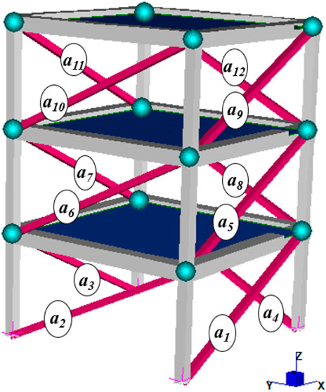
FIGURE 3. Case study 2: global view of the structure with indication of the position of the unknown parameters a₁–a₁₂.

The structure has been modeled by introducing the membrane rigid floor hypothesis for story slabs and, so, the structure has nine DOF (two translations in X and Y respectively and one rotation along the vertical axis Z for each story). The natural frequencies and the corresponding modal participating mass ratios of the building have been evaluated and summarized in Table 2.

TABLE 2

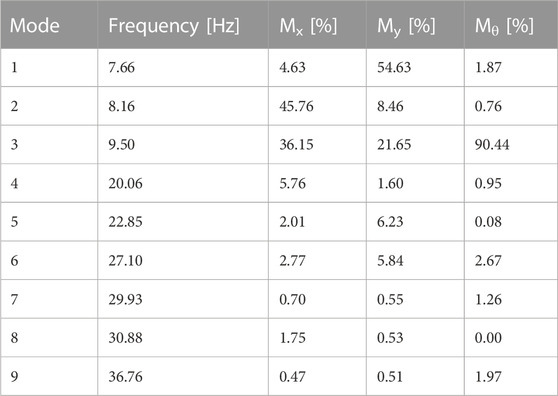
TABLE 2. Case study 2: natural frequencies and respective modal participating mass ratios.

Five different scenarios have been considered, assuming alternatively 12, 10, 8, 6, and 4 parameters to be evaluated. For all the scenarios, the model updating procedure is performed alternatively adopting 2, 3, 4, 5, or 9 natural frequencies and respective mode shapes, obtaining 25 cases in total. The CoV of frequencies and mode shape components is assumed equal to 5%, for all the vibrating modes. To validate the results obtained by means of the two-step procedure, the different CoVs are computed. For all the cases, a Monte Carlo simulation is performed by considering 500 realizations.

Figure 4 shows the CoV of the unknown multipliers a₁ and a₄ for different combinations of vibrating modes adopted in the procedure and the number of unknown parameters to identify. It is worth noting that the CoV of a parameter monotonically decreases if the number of adopted modes increases. Moreover, the uncertainty of a specific parameter is almost insensitive to the total number of parameters introduced in the procedure. The CoV of the unknown parameters is very high if a few modes (i.e. 2, 3) are selected, with values ranging from 20% to 80%. With a set of data considering more than 4 vibrating modes, the CoV is smaller than 20% for all the analyzed cases. Finally, considering 9 vibrating modes, the CoV of parameters reaches the minimum value of about 8%. It is worth highlighting that for some parameters, there is a negligible improvement in the uncertainty evaluation even if the number of considered vibrating modes is greater than 5 (see for instance the parameter a₄ in Figure 3). In any case, starting from a typical CoV value affecting the frequencies and the mode shape components (i.e. 5%), the CoV of unknown parameters was much higher, showing that structural parameters give, in general, more scattered results than the modal parameters adopted as input (frequencies and mode shape components). Consequently, when the procedure also aims to quantify structural mechanical parameter values, particular attention must be paid to the input dataset size, especially if low-sensitive parameter values are to be evaluated.

FIGURE 4

FIGURE 4. CoV for different combinations of adopted vibrating modes and unknown parameters: results for the parameters a₁ and a₄ for the scenarios considering 4, 6 and 12 unknown parameters.

Finally, Figure 5 shows the comparison between the values of CoV provided by the present procedure (solid line) and Monte Carlo (dashed line) simulation for the unknown parameter a₂. The figure confirms, also for this case study, the good agreement of the results coming from the two different methods and, for the case at hand, if the number of considered modes is greater than four, the two procedures provide the same CoV values. Similar trends are obtained for the other parameters (not shown in the figure).

FIGURE 5

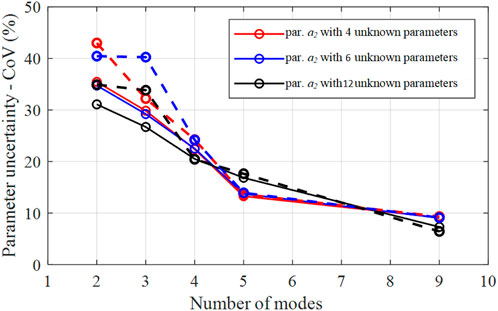
FIGURE 5. CoV for different combinations of adopted vibrating modes and unknown parameters: comparison between the results provided by the proposed procedure (solid line) and Monte Carlo simulation (dashed line) for unknown parameter a₂.

5 Damage assessment of a three-story real building

5.1 Description of structure, induced damage, tests, and instrumentation

The structure is an RC-framed building with masonry infill panels constructed in the 1920s in El Centro, California. The construction, named the “El Centro building” (see Figure 6A), included the basement, the ground floor, and the first floor, with plan dimensions of 27.0 m × 32.3 m. The structure had RC frames in the North-South direction connected by arch-type joists in the East-West direction. The structure was damaged by three major earthquakes striking the area in 1940, 1979, and 1987 and was retrofitted in the late 1980s. The retrofit focused on the strengthening of the masonry infills along the perimeter frames of the ground floor.

FIGURE 6

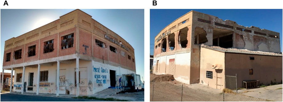
FIGURE 6. El Centro building (Yousenfianmoghadam et al., 2015). (A) Global view; (B) Picture of the building at the end of the tests after the demolition of four infill panels at the first floor.

During the 2010 Baja California Earthquake, the first-floor infills and the perimeter frames in the North, West, and South sides were severely damaged while the East side did not exhibit any visible crack or detriment. The building was tested in the nonlinear range of response using mobile shakers at three different damage levels, or damage states, labeled DS₂, DS₃, and DS₄, introduced by the additional destruction of some perimeter infills of the first floor: three on the West side and one on the South side (Yousenfianmoghadam et al., 2015). All three damaged states and the undamaged state (DS₁) are considered in this study. Figure 6B shows the building at the end of the tests after the demolition of four infill panels in the first story. The location and the sequence for wall removal are shown in Figure 7A. An array of 60 accelerometers was installed close to the four corners and at the center of the slab on each floor and measured accelerations in three directions at every location. The selected instrumentation allowed the identification of the translational and torsional vibrating modes of the building. The acceleration response of the building to ambient excitations was recorded for 120 h using a data logger, which could record accelerations between 0.1 mg and 2 g with a sampling rate of 200 Hz. More information about the tests on the structure, its design details, and in-depth details on the response to the testing sequence can be found in Yousenfianmoghadam et al. (2015).

FIGURE 7

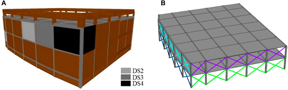
FIGURE 7. Global view of (A) infill removal sequence associated to the different damage states DS and (B) FE model adopted for the study of the El Centro building.

The two-step procedure proposed here was adopted to identify the in-plane stiffness of the infill panels, located on each side of the first story resulting in four unknown parameters to be updated.

The geometry and the material properties of structural and non-structural elements are assumed according to Yousenfianmoghadam et al. (2015). The numerical FE model adopted for the numerical simulation is depicted in Figure 7B and it is obtained with OpenSEES software (Opensees, 2016). The structural model of the RC frames is obtained by means of mono-dimensional beam elements. The slabs have been modeled by 4-node shell elements with the equivalent membrane and flexural thickness. To maintain simplicity in the numerical model as much as possible, the masonry infills between consecutive columns are introduced in the FE model by two equivalent diagonal truss elements following the modeling framework proposed in Bose et al. (2018). The parameters to identify a_i are multipliers of the axial rigidity S = a∙E·A of the equivalent diagonal struts of the first floor, arranged as illustrated in Figure 8 (where E: masonry Young modulus; A: equivalent strut cross-section area; a: multiplier to identify). The stiffness values of the infill panels at both the ground and underground stories are obtained by using the methodology proposed in Stavridis (2009). The estimated stiffness is reduced by means of two reduction factors to take into account the openings and existing damage in the infill panels, according to the damage detection realized before the experimental campaign (Song et al., 2018).

FIGURE 8

FIGURE 8. Plan view of the first floor of the El Centro building, showing the unknown parameters arrangement for the infill modelling.

To obtain the matrices ${\mathit{K}}_s$ defined in Eq. 1, the following difference is considered:

${\mathit{K}}_s={\overline{\mathit{K}}}_s-{\mathit{K}}_0(52)$

where: ${\overline{\mathbf{K}}}_s$ is the global stiffness matrix obtained assigning to the s-th parameter a unitary value and zero for the other parameters, and K₀ is the stiffness matrix with all parameters set equal to zero.

To perform the model updating procedure, the first two natural vibrating modes are considered in this study, with the weight parameters p₁ and p₂ set equal to 1.0. The mode shape components are statically condensed, introducing the rigid diaphragm assumption, into three components for each story, i.e., translation in X and Y direction and rotation around vertical axis Z, with axis reference system positioned at the story center of mass and with Y axis coincident with North direction. The assumption of a rigid diaphragm is justified by the high stiffness of the existent slabs with respect to the frame, and the low level of excitation reached during the ambient vibration tests.

The proposed two-step procedure is applied to the four states (DS₁-DS₄), allowing for the evaluation of the updated rigidity values S_i = a_i·E·A_i reported in Table 3. The comparison between experimental and numerical frequencies and mode shapes is reported in Table 4. The modal assurance criterion (MAC) (Clough et al., 1995) values for the different DS are higher than 0.97. That means that there exists an almost perfect correspondence between experimental and numerical mode shapes. Moreover, the relative errors in the frequency estimations were very low, proving the high reliability of the numerical procedure.

TABLE 3

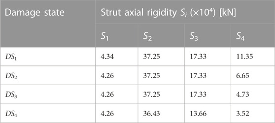
TABLE 3. El Centro building: axial rigidities S_i (with S = a∙E·A) of the equivalent struts simulating the infill panels, as identified by the two-step procedure for the different damage states DS₁–DS₄.

TABLE 4

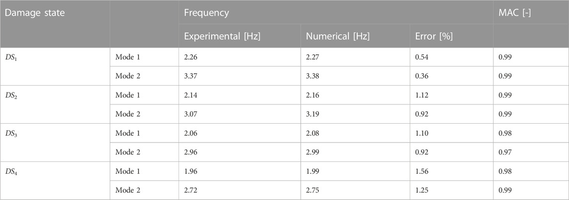
TABLE 4. El Centro building: experimental and numerical frequencies, frequency relative errors and MAC for the damage states DS₁ - DS₄.

To quantify the expected damage for the various infill panels, the Damage Index (Tondi et al., 2019) E_i has been defined as:

$E_i\left({DS}_j\right)=\frac{a_i\left({DS}_1\right)-a_i\left({DS}_j\right)}{a_i\left({DS}_1\right)}(53)$

where: a_i (DS_j) is the multiplier value identified for the i-th unknown parameter in the j-th damage state DS_j. With this definition, the damage index E_i ranges from 0.0 (for undamaged components) to 1.0 (for completely damaged members). The values of the Damage Index are reported in Table 5 for the different unknown parameters and for each damage state DS₂-DS₄.

TABLE 5

TABLE 5. Evaluation of the Damage Index for increasing damage levels (DS₂-DS₄) calculated for each unknown parameter.

The obtained damage indices established a numerical “virtual” scenario that matches very well with the actual scenario of degradation, for all the increasing damage levels, and shows the ability of the technique to properly identify the position of the damaged infills. The damage indices associated with multipliers $a_1$ and $a_2$ are close to zero for all the damage states which is consistent with the removal procedure since no wall was demolished on the North and East sides. Correctly, the damage index E₃ is close to zero in DS₂ and DS₃, and it increases in damage state DS₄ when one infill panel was demolished on the South side. Finally, the damage index E₄ of the multiplier a₄ properly represents the progressive removal on the West side where an infill panel has been removed at every damage state from DS₂ to DS₄.

5.2 Parameter uncertainty assessment

The procedure presented in Section 3 has been applied to assess the uncertainties related to the rigidity parameters S₁–S₄, identified for the different damage states. The procedure suggested by Reynders (Reynders et al., 2008) has been applied in order to calculate the covariance matrix of the experimental modal parameters. The experimental CoV of the frequencies is rather small, in the range of 3%–4%, while the CoV of the mode shapes components is higher, ranging from 10% to 40%. The main outcomes of the procedure, reported in terms of mean value, standard deviation, and CoV values of the strut axial rigidity containing the unknown parameters have been collected in Table 6. The results show a very high variability for the parameters, with CoV up to 202% in one particular case. The wide scattering of the identified parameters is mainly due to the large uncertainty values of mode shape components resulting from in-situ experimental tests. Ideally, if the uncertainty affecting the mode shape components could be reduced, the CoV of the unknown parameters should be strongly reduced. For instance, if we assume for the mode shape components an ideal CoV value equal to 8%, the new scenario would become the one shown in Table 7. In the ideal condition, the maximum CoV of the unknown parameters should be reduced from the original 202%–35%, and in general, the new ideal results show a moderate parameter variability with CoV in the range 9%–35%.

TABLE 6

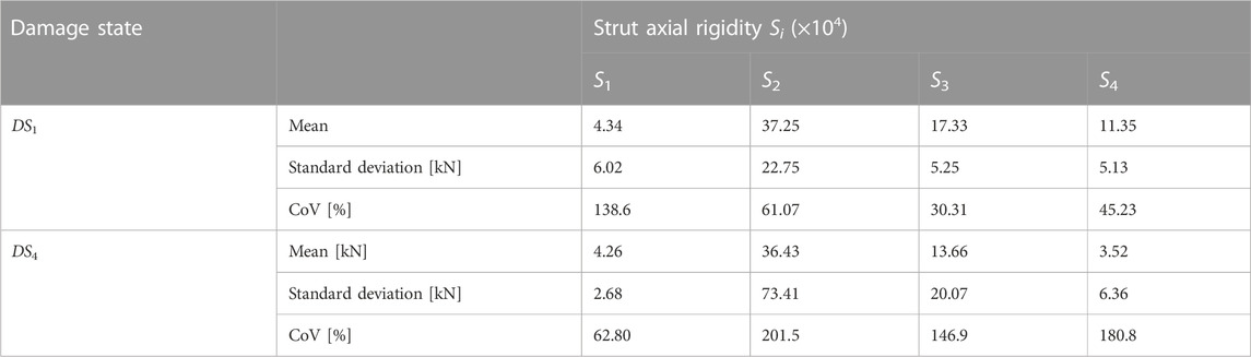
TABLE 6. Mean values, standard deviations, and CoVs of the four equivalent strut rigidities S₁-S₄ calculated for the El Centro building for damage states DS₁ and DS₄, starting from the experimental data available for the El Centro building.

TABLE 7

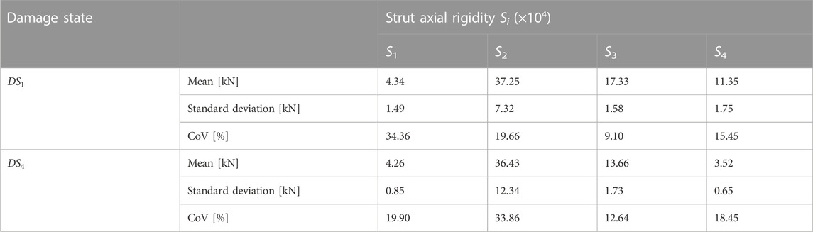
TABLE 7. Mean values, standard deviations, and CoVs of the four equivalent strut rigidities S₁–S₄ calculated for the El Centro building for damage states DS₁ and DS₄, starting from the experimental data of frequencies assuming a CoV value equal to 8% for the mode shape components.

Therefore, in the mechanical parameter uncertainty evaluation, great importance is attributed to the mode shape uncertainties. For the case investigated here, a little variation in a mode shape produces high modification to both in-plane and elevation story stiffness distribution and, therefore, a large variability of the strut rigidity values. This real case study confirms that the unknown parameters of a structure (i.e., the output of the procedure), governing the dynamic behavior of the building, are much more scattered than the considered modal parameters (i.e., the input in the procedure).

6 Conclusion

This article presents an efficient and fast two-step procedure for the evaluation of unknown parameters and their uncertainties in the context of dynamic model updating. In the first step, the least square problem is solved in order to obtain an estimate of the mechanical parameters governing the behavior of the structural system. The target function is composed of the residuals of the dynamic eigenvalues problem and the input parameters are the natural frequencies and mode shape components of the structures. A second iterative step improves the final solution if the first step does not achieve the prescribed desired tolerance. Moreover, by exploiting the error propagation theory, a direct procedure is also presented in order to assess the parameter uncertainty starting from the covariance matrix of the considered frequencies and mode shape components.

The computational effort needed to obtain a reliable numerical solution is important if the results and the damage assessment are required in real-time or quasi-real-time, as for health monitoring systems adopted to evaluate the unsafe/safe state of a structure during its service life or in the aftermath of a catastrophic event. Moreover, the assessment of the unknown parameter uncertainty has significant relevance especially if the decision-maker has to decide to close a bridge or a building to prevent human losses in case of structural collapse.

The first step of the proposed methodology allows one to immediately find a reliable estimate of the unknown parameters and the corresponding uncertainties so that the decision-maker can immediately have information on the structural health. Moreover, if needed, the second step produces a more refined solution in terms of both unknown parameters and corresponding uncertainty values.

The methodology was applied to two numerical examples to test the reliability of the method. Then the procedure was adopted for the damage assessment of a three-story full-scale existing building, experimentally tested by introducing progressive damage to the masonry infill panels. As expected, the results show that starting from a limited number of available vibrating modes, even if the COV of the modal parameters is low, the uncertainties of the mechanical/geometrical parameters to assess are much higher. The results highlight that the unknown structural parameters are much more scattered than the modal data used as input. Consequently, when the model updating procedure is aimed to quantify the parameter values governing the structural system, particular attention must be paid to the uncertainties in input data and especially to the mode shape components.

Data availability statement

All data reported in Section 4 will be made available by the authors, without undue reservation. The data analyzed in Section 5 was obtained from Yousenfianmoghadam et al. (2015). Requests to access these datasets should be directed to the authors.

Author contributions

MT: Conceptualization, Data curation, Software, Writing–original draft. MB: Conceptualization, Formal Analysis, Validation, Writing–review and editing. LV: Conceptualization, Supervision, Validation, Writing–review and editing.

Funding

The author(s) declare that no financial support was received for the research, authorship, and/or publication of this article.

Conflict of interest

Author MT was employed by IN20 s.r.l.

The remaining authors declare that the research was conducted in the absence of any commercial or financial relationships that could be construed as a potential conflict of interest.

Publisher’s note

All claims expressed in this article are solely those of the authors and do not necessarily represent those of their affiliated organizations, or those of the publisher, the editors and the reviewers. Any product that may be evaluated in this article, or claim that may be made by its manufacturer, is not guaranteed or endorsed by the publisher.

References

Beck, J., and Katafygiotis, L. (1998). Updating models and their uncertainties, I: bayesian statistical framework. ASCE J. Eng. Mech. 124 (4), 455–461. doi:10.1061/(asce)0733-9399(1998)124:4(455)

CrossRef Full Text | Google Scholar

Berger, M. (1987). Geometry I. Berlin, Germany: Springer-Verlag.

Google Scholar

Bose, S., Tempestti, J. M., and Stavridis, A., (June 2018) Framework for the nonlinear dynamic simulation of the seismic response of infilled RC frames. In: Proceedings of the 11th national conference on earthquake engineering. Los Angeles, California, United States.

Google Scholar

Bursi, O. S., Kumar, A., Abbiati, G., and Ceravolo, R. (2014). Identification, model updating, and validation of a steel twin deck curved cable-stayed footbridge. Comput-Aid Civ. Infrastruct. Eng. 29, 703–722. doi:10.1111/mice.12076

CrossRef Full Text | Google Scholar

Bursi, O. S., Zonta, D., Debiasi, E., and Trapani, D. (2018). Structural health monitoring for seismic protection of structure and infrastructure systems. Berlin, Germany: Springer, 339–358.

CrossRef Full Text | Google Scholar

Caicedo, J. M., and Yun, G. (2011). A novel evolutionary algorithm for identifying multiple alternative solutions in model updating. Struct. Health Monit. 10 (5), 491–501. doi:10.1177/1475921710381775

CrossRef Full Text | Google Scholar

Ching, J., and Beck, J. L. (2004). New bayesian model updating algorithm applied to a structural health monitoring benchmark. Struct. Health Monit. 3 (4), 313–332. doi:10.1177/1475921704047499

CrossRef Full Text | Google Scholar

Christodoulou, K., and Papadimitriou, C. (2007). Structural identification based on optimally weighted modal residuals. Mech. Syst. Signal Process. 21 (1), 4–23. doi:10.1016/j.ymssp.2006.05.011

CrossRef Full Text | Google Scholar

Clough, R. W., and Penzien, J. (1995). Dynamics of structures. Berkeley, CA, USA: Computers & Structures, Inc.

Google Scholar

Coleman, T. F., and Li, Y. (1996). An interior, trust region approach for nonlinear minimization subject to bounds. SIAM J.Optim. 6 (2), 418–445. doi:10.1137/0806023

CrossRef Full Text | Google Scholar

Conn, A. R., Gould, N. I. M., and Toint, P. L. (2000). Trust-region methods, MOS-SIAM series on optimization. Philadelphia, PA, USA: Society for Industrial and Applied Mathematics.

Google Scholar

Degrauwe, D., De Roeck, G., and Lombaert, G. (2009). Uncertainty quantification in the damage assessment of a cable-stayed bridge by means of fuzzy numbers. Comput. Struct. 87 (17-18), 1077–1084. doi:10.1016/j.compstruc.2009.03.004

CrossRef Full Text | Google Scholar

Doebling, S. W., Farrar, C. R., and Prime, M. B. (1998). A summary review of vibration-based damage identification methods. Shock Vib. Dig. 30 (2), 91–105. doi:10.1177/058310249803000201

CrossRef Full Text | Google Scholar

Fan, W., and Qiao, P. (2010). Vibration-based damage identification methods: a review and comparative study. Struct. Health Monit. 10 (1), 83–111. doi:10.1177/1475921710365419

CrossRef Full Text | Google Scholar

Goller, B., and Schueller, G. I. (2011). Investigation of model uncertainties in Bayesian structural model updating. J. sound Vib. 330 (25), 6122–6136. doi:10.1016/j.jsv.2011.07.036

PubMed Abstract | CrossRef Full Text | Google Scholar

Lang, S. (2002). Algebra. 3rd Edition. New York, NY, USA: Springer-Verlag.

Google Scholar

Lang, S. (2005). Undergraduate algebra. 3rd Edition. New York, NY, USA: Springer-Verlag.

Google Scholar

MathWorks, (2023). Matlab: high performance numeric computation and visualization software, User’s Guide. Natick, MA, USA: MathWorks Inc.

Google Scholar

Mottershead, J. E., and Friswell, M. I. (1993). Model updating in structural dynamics: a survey. J. Sound Vib. 167, 347–375. doi:10.1006/jsvi.1993.1340

CrossRef Full Text | Google Scholar

Nguyen, A., Kodikara, K. T. L., Chan, T. H., and Thambiratnam, D. P. (2019). Deterioration assessment of buildings using an improved hybrid model updating approach and long-term health monitoring data. Struct. Health Monit. 18 (1), 5–19. doi:10.1177/1475921718799984

CrossRef Full Text | Google Scholar

Opensees, (2016). OpenSEES. http://opensees.berkeley.edu (Accessed January 15, 2020).

Google Scholar

Ponsi, F., Bassoli, E., and Vincenzi, L. (2021). A multi-objective optimization approach for FE model updating based on a selection criterion of the preferred Pareto-optimal solution. Structures 33, 916–934. doi:10.1016/j.istruc.2021.04.084

CrossRef Full Text | Google Scholar

Ponsi, F., Bassoli, E., and Vincenzi, L. (2022). Bayesian and deterministic surrogate-assisted approaches for model updating of historical masonry towers. J. Civ. Struct. Health Monit. 12 (6), 1469–1492. doi:10.1007/s13349-022-00594-0

CrossRef Full Text | Google Scholar

Reynders, E., Pintelon, R., and De Roeck, G. (2008). Uncertainty bounds on modal parameters obtained from stochastic subspace identification. Mech. Syst. signal Process. 22 (4), 948–969. doi:10.1016/j.ymssp.2007.10.009

CrossRef Full Text | Google Scholar

Simoen, E., Papadimitriou, C., and Lombaert, G. (2013). On prediction error correlation in Bayesian model updating. J. Sound Vib. 332 (18), 4136–4152. doi:10.1016/j.jsv.2013.03.019

CrossRef Full Text | Google Scholar

Song, M., Yousefianmoghadam, S., Mohammadi, M. E., Moaveni, B., Stavridis, A., and Wood, R. L. (2018). An application of finite element model updating for damage assessment of a two-story reinforced concrete building and comparison with lidar. Struct. Health Monit. 17 (5), 1129–1150. doi:10.1177/1475921717737970

CrossRef Full Text | Google Scholar

Stavridis, A. (2009). Analytical and experimental seismic performance assessment of masonry-infilled RC frames. Ph.D. thesis. San Diego, CA, USA: University of California.

Google Scholar

Taylor, J. R. (1997). An introduction to error analysis: the study of uncertainties in physical measurements. Melville, NY, USA: University Science Books.

Google Scholar

Teughels, A., and De Roeck, G. (2004). Structural damage identification of the highway bridge Z24 by FE model updating. J. Sound Vib. 278 (3), 589–610. doi:10.1016/j.jsv.2003.10.041

CrossRef Full Text | Google Scholar

Teughels, A., Maeck, J., and De Roeck, G. (2002). Damage assessment by FE model updating using damage functions. Comput. Struct. 80 (25), 1869–1879. doi:10.1016/s0045-7949(02)00217-1

CrossRef Full Text | Google Scholar

Tondi, M. (2018). Innovative model updating procedure for dynamic identification and damage assessment of structures. PhD Thesis. Italy: University of Bologna.

Google Scholar

Tondi, M., Yousenfianmoghadam, S., Stavridis, A., Moaveni, B., and Bovo, M. (2019). “Model updating and damage assessment of RC structure using an iterative eigenvalue problem,” in Dynamics of Civil Structures, Volume 2. Conference Proceedings of the Society for Experimental Mechanics Series, Editor S. Pakzad, Springer, Cham. doi:10.1007/978-3-319-74421-6_47

CrossRef Full Text | Google Scholar

Vahedi, M., Khoshnoudian, F., and Hsu, T. Y. (2018). Application of Bayesian statistical method in sensitivity-based seismic damage identification of structures: numerical and experimental validation. Struct. Health Monit. 17 (5), 1255–1276. doi:10.1177/1475921718783360

CrossRef Full Text | Google Scholar

Vincenzi, L., and Gambarelli, P. (2017). A proper infill sampling strategy for improving the speed performance of a Surrogate-Assisted Evolutionary algorithm. Comput. Struct. 178, 58–70. doi:10.1016/j.compstruc.2016.10.004

CrossRef Full Text | Google Scholar

Vincenzi, L., and Simonini, L. (2017). Influence of model errors in optimal sensor placement. J. Sound Vib. 389, 119–133. doi:10.1016/j.jsv.2016.10.033

CrossRef Full Text | Google Scholar

Yousenfianmoghadam, S., Song, M., Stavridis, A., and Moaveni, B. (December 2015) System identification of a two-story infilled RC building in different damage states. In: Proceedings of the improving the seismic performance of existing buildings and other structures 2015, San Francisco, CA, USA.

Google Scholar

Zarate, B. A., and Caicedo, J. M. (2008). Finite element model updating: multiple alternatives. Eng. Struct. 30 (12), 3724–3730. doi:10.1016/j.engstruct.2008.06.012

CrossRef Full Text | Google Scholar

Zhang, Q. W. (2007). Statistical damage identification for bridges using ambient vibration data. Comput. Struct. 85 (7-8), 476–485. doi:10.1016/j.compstruc.2006.08.071

CrossRef Full Text | Google Scholar

Zheng, Z. D., Lu, Z. R., Chen, W. H., and Liu, J. K. (2015). Structural damage identification based on power spectral density sensitivity analysis of dynamic responses. Comput. Struct. 146, 176–184. doi:10.1016/j.compstruc.2014.10.011

CrossRef Full Text | Google Scholar

Appendix

In order to prove Eq. 26, the eigenvalues/eigenvectors dynamic problem is considered in its standard form:

$\left(\mathit{K}-{\omega }_i^2\mathit{M}\right){\mathit{\phi }}_i=\mathbf{0}(\mathrm{A1})$

with: $\mathit{K},\mathit{M}\in S^{mxm},D^{+}$ are symmetric and positive definite matrices, ${\omega }_i^2$ is the i-th square circular frequency (i.e., i-th eigenvalue) and ${\varphi }_i\in R^m$ is the i-th mode shape vector. The system Eq. A1 can be rewritten as follows:

$\left(\sqrt{\mathit{M}}\left[\sqrt{{\mathit{M}}^{-1}}\mathit{K}\sqrt{{\mathit{M}}^{-1}}-{\omega }_i^2{\mathit{I}}^{mxm}\right]\sqrt{\mathit{M}}\right){\mathit{\phi }}_i=\mathbf{0}\forall i(\mathrm{A2})$

where: ${\mathit{I}}^{mxm}$ is the identity matrix of order m. After:

$\left[\sqrt{{\mathit{M}}^{-1}}\mathit{K}\sqrt{{\mathit{M}}^{-1}}-{\omega }_i^2{\mathit{I}}^{mxm}\right]{\widehat{\mathit{\phi }}}_i=\mathbf{0}\forall i(\mathrm{A3})$

where: ${\widehat{\mathit{\phi }}}_i=\sqrt{\mathit{M}}{\mathit{\phi }}_i$. Then, it is stated that:

$\widehat{\mathit{K}}=\sqrt{{\mathit{M}}^{-1}}\mathit{K}\sqrt{{\mathit{M}}^{-1}}(\mathrm{A4})$

where: $\widehat{\mathit{K}}$ is a positive definite and symmetric matrix (Lang, 2002; Lang, 2005). Thus, the problem Eq. A1 can be rewritten as:

$\left[\widehat{\mathit{K}}-{\omega }_i^2{\mathit{I}}^{mxm}\right]{\widehat{\mathit{\phi }}}_i=\mathbf{0}\forall i(\mathrm{A5})$

Equation A5 represents a standard eigenvalues problem. Using the Spectral Theorem (Lang, 2002; Lang, 2005), the matrix $\widehat{\mathit{K}}$ can be decomposed using its eigenvectors and eigenvalues:

$\widehat{\mathit{K}}=\widehat{\mathit{P}}\mathit{\Lambda }{\widehat{\mathit{P}}}^{-1}(\mathrm{A6})$

in which: $\widehat{\mathit{P}}\in R^{mxm}$ is the matrix whose columns represent the eigenvectors ${\widehat{\mathit{\phi }}}_i$; $\mathit{\Lambda }\in R^{mxm}$ is a diagonal matrix collecting the eigenvalues in its leading diagonal:

$\mathit{\Lambda }=\left[\begin{array}{cccc}{\omega }_1^2& 0& \cdots & 0\\ 0& {\omega }_2^2& \cdots & 0\\ ⋮& ⋮& \ddots & 0\\ 0& 0& 0& {\omega }_m^2\end{array}\right](\mathrm{A7})$

The matrix $\widehat{\mathit{K}}$ is symmetric and, for the Spectral Theorem, the matrix $\widehat{\mathit{P}}\in O^{mxm}$ is an orthogonal matrix. Thus, it is possible to impose the following normalization:

${\widehat{\mathit{\phi }}}_i^T{\widehat{\mathit{\phi }}}_j={\mathit{\delta }}_{ij}(\mathrm{A8})$

where ${\delta }_{ij}$ is the Kronecker delta. Therefore, Equation A8 can be rewritten as:

${\left(\sqrt{\mathit{M}}{\mathit{\phi }}_j\right)}^T\left(\sqrt{\mathit{M}}{\mathit{\phi }}_j\right)={\delta }_{ij}(\mathrm{A9})$

with

$\left\{\sqrt{\mathit{M}}{\mathit{\phi }}_1\right.,\sqrt{\mathit{M}}{\mathit{\phi }}_2,\cdots ,\sqrt{\mathit{M}}\left.{\mathit{\phi }}_m\right\}(\mathrm{A10})$

representing a base of the subspace ${\mathfrak{R}}^m$. Then, from Equation A4, the stiffness matrix can be expressed in the following form:

$\mathit{K}=\sqrt{\mathit{M}}\widehat{\mathit{P}}\mathit{\Lambda }{\widehat{\mathit{P}}}^T\sqrt{\mathit{M}}(\mathrm{A11})$

Changing the notation with:

$\widehat{\mathit{P}}=\sqrt{\mathit{M}}\mathit{P}(\mathrm{A12})$

where: $\mathit{P}\in R^{mxm}$ is the matrix whose i-th column represents the eigenvector of the original generalized eigenvalues/eigenvectors problem, Equation A11 can be posed in the form:

$\mathit{K}=\mathit{M}\mathit{P}\mathit{\Lambda }{\left(\mathit{M}\mathit{P}\right)}^T(\mathrm{A13})$

From Eq. A13 it is possible to evaluate the maximum number of identifiable parameters for a problem having a size equal to m when n eigenvalues/eigenvectors are available. If only n pairs of eigenvalues and eigenvectors are available, with $1\le n\le m$:

$\left({\omega }_1^2,{\mathit{\phi }}_1\right);\cdots ;\left({\omega }_n^2,{\mathit{\phi }}_n\right)(\mathrm{A14})$

The quantity:

$\left\{\sqrt{\mathit{M}}{\mathit{\phi }}_1\right.,\sqrt{\mathit{M}}{\mathit{\phi }}_2,\cdots ,\sqrt{\mathit{M}}\left.{\mathit{\phi }}_n\right\}(\mathrm{A15})$

represents a base of the subspace ${\mathfrak{R}}^n$. In order to complete the base of the space of order m, a set of m-n vectors must be defined. This can be done in the following way:

$\left\{\sqrt{\mathit{M}}{\mathit{\phi }}_1,\sqrt{\mathit{M}}{\mathit{\phi }}_2,\cdots ,\sqrt{\mathit{M}}{\mathit{\phi }}_{\mathit{n}},\sqrt{\mathit{M}}{\mathit{\phi }}_{n+1}^{\prime },\cdots ,\sqrt{\mathit{M}}{\mathit{\phi }}_m^{\prime }\right\}$

Thus, the matrices $\widehat{\mathit{P}}$ and $\mathit{\Lambda }$ can be rewritten as:

$\widehat{\mathit{P}}=\left[\sqrt{\mathit{M}}{\mathit{\phi }}_1,\sqrt{\mathit{M}}{\mathit{\phi }}_2,\cdots ,\sqrt{\mathit{M}}\left.{\mathit{\phi }}_n\right|\sqrt{\mathit{M}}{\mathit{\phi }}_{n+1}^{\prime },\cdots ,\sqrt{\mathit{M}}{\mathit{\phi }}_m^{\prime }\right](\mathrm{A17})$

$\mathit{\Lambda }=\left[\begin{array}{cc}{\mathit{\Lambda }}_n& \mathbf{0}\\ \mathbf{0}& {\mathit{\Lambda }}_{m-n}^{\prime }\end{array}\right](\mathrm{A18})$

in which:

${\mathit{\Lambda }}_n=\left[\begin{array}{cccc}{\omega }_1^2& 0& \cdots & 0\\ 0& {\omega }_2^2& \cdots & 0\\ ⋮& ⋮& \ddots & 0\\ 0& 0& 0& {\omega }_n^2\end{array}\right](\mathrm{A19})$

${\mathit{\Lambda }}_{m-n}^{\prime }\in S^{\left(m-n\right)x\left(m-n\right)}$ is a positive definite symmetric matrix. The stiffness matrix $\mathit{K}$ can be expressed as:

$\mathit{K}=\sqrt{\mathit{M}}\widehat{\mathit{P}}\left[\begin{array}{cc}{\mathit{\Lambda }}_n& \mathbf{0}\\ \mathbf{0}& {\mathit{\Lambda }}_{m-n}^{\prime }\end{array}\right]{\widehat{\mathit{P}}}^T\sqrt{\mathit{M}}(\mathrm{A20})$

or, alternatively:

$\mathit{K}=\sqrt{\mathit{M}}\widehat{\mathit{P}}\left[\begin{array}{cc}{\mathit{\Lambda }}_n& \mathbf{0}\\ \mathbf{0}& \mathbf{0}\end{array}\right]{\widehat{\mathit{P}}}^T\sqrt{\mathit{M}}+\sqrt{\mathit{M}}\widehat{\mathit{P}}\left[\begin{array}{cc}\mathbf{0}& \mathbf{0}\\ \mathbf{0}& {\mathit{\Lambda }}_{m-n}^{\prime }\end{array}\right]{\widehat{\mathit{P}}}^T\sqrt{\mathit{M}}(\mathrm{A21})$

Therefore, $\mathit{K}$ represents an affine subspace having order o = $\frac{\left(m-n\right)\cdot \left(m-n+1\right)}{2}$, that is the same order of unknowns in matrix ${\mathit{\Lambda }}_{m-n}^{\prime }$. Following the procedure described in Section 2, matrix $\mathit{K}$ can be decomposed as follows:

$\mathit{K}={\mathit{K}}_0+{\displaystyle \sum _{s=1}^N}{a}_s{\mathit{K}}_s(\mathrm{A22})$

that is an affine subspace of order N. Introducing the theorem on affine spaces (Berger, 1987; Lang, 2002; Lang, 2005), the following relation between subspaces (Eqs A20, A21) can be set:

$N+\frac{\left(m-n\right)\cdot \left(m-n+1\right)}{2}-\frac{m\cdot \left(m+1\right)}{2}\left\{\begin{array}{cc}>0& \text{Infinite}\hspace{0.33em}\text{solutions}\\ =0& \text{Exact}\hspace{0.33em}\text{solution}\\ <0& \text{Optimal}\hspace{0.33em}\text{solution}\end{array}\right.(\mathrm{A23})$

where: $\frac{m\cdot \left(m+1\right)}{2}$ is the number of parameters in a symmetric matrix of order m. Therefore, the maximum number N of identifiable parameters is:

$N=\frac{m\cdot \left(m+1\right)}{2}-\frac{\left(m-n\right)\cdot \left(m-n+1\right)}{2}(\mathrm{A24})$

or:

$N=n\cdot \left(m+1\right)-{\displaystyle \sum _{i=1}^n}i(\mathrm{A25})$