Statistical assessment of the wave loads at walls through two-phase CFD modeling of the effects of air compressibility

1 Introduction

The accurate representation of the wave–structure interaction is fundamental to assess the design wave load and the performance of coastal defenses. However, it still represents a challenging task, due to the highly turbulent flow conditions, the non-linear dynamics, and the occurrence of wave breaking and of air entrainment (Aleixo et al., 2018; Raby et al., 2020; Stringari et al., 2021).

Many studies experimentally demonstrated the relevance of air pockets on the distribution and on the intensity of the wave pressures at seawalls consequent to wave impacts (a.o. Peregrine et al., 2005; Cuomo et al., 2010a; Plumerault et al., 2012a; Bredmose et al., 2015; Formentin et al., 2021a). Air bubbles can be entrapped beneath the breaker if the wave overturns just before the wall, whereas large quantities of air can be entrained in the water phase if the wave has already broken, determining a turbulent air–water mixture striking the wall. In both cases, the compressibility of the entrained air will affect the dynamics, and though it might reduce the maximum pressure due to a cushioning effect, it will also tend to distribute the impact pressures more widely so that the overall force on the wall may not be reduced (Peregrine et al., 2005) and the impulse may be increased due to rebound (Wood et al., 2000).

The experimental investigation of the air entrapment is complicated for both practical and economic reasons. The aeration induces non-negligible scale effects, that may introduce errors to various degrees during the scaling process from model to prototype conditions (Mitsuyasu, 1967; Takahashi et al., 1985; Cuomo et al., 2010a; Bredmose et al., 2015). On the other hand, large-scale experiments to avoid or reduce scale effects often cannot be pursued because of the unfeasible time and economic investment.

In such a context, numerical simulations represent a good alternative as they limit scale effects and do not introduce measurement errors (Liu et al., 2019). However, numerical models are affected by numerical errors, which depend on the numerical scheme, filters, grid resolution, turbulence model, time step, etc. (a.o. Toro, 2002; Rogers et al., 2002; Gullbrand and Katopodes Chow, 2003; Olsson, 2017; Wang et al., 2018; Lloyd et al., 2020). The choices of the modelers can lead, therefore, to more realistic and accurate results or can introduce systematic errors instead.

Within the phase-resolving class of wave models, those that resolve the vertical flow structure and solve the fully non-linear, time-averaged Navier–Stokes (NS) equations—often referred to as computational fluid dynamics (CFD) or depth-resolving models—have the least theoretical limitations and are generally considered the most accurate. CFD models, such as the mesh-based Eulerian approach OpenFOAM (Jasak et al., 2007) or mesh-less Lagrangian approach DualSPHysics (Crespo et al., 2015), are able to simulate complex processes including wave–structure interaction from deep to shallow water conditions. Plumerault et al. (2012a) and Ma et al. (2014) estimated the impact of plunging breakers against a vertical wall by means of a multi-fluid compressible Navier–Stokes model and in a low-filling depressurized sloshing tank. Liu et al. (2019) simulated breaking wave impacts on a vertical wall using a two-dimensional two-phase CFD model, where the air was considered an iso-entropic ideal gas and water was treated as an incompressible liquid. Simonetti et al. (2018) made use of a compressible two-phase CFD model in the OpenFOAM environment to simulate a fixed oscillating water column device to assess the scale effects associated to air compressibility. Boshi and Ketabdari (2021) introduced the cut-cell method to porous media, reducing the computational cost of modeling the sloped boundaries of structures to obtain a sensible comprehension of solitary wave interaction with an emerged porous breakwater. Saghi et al. (2022) numerically investigated the hydrodynamic efficiency of floating breakwaters by coupling the fast fictitious domain method with the classic volume of fluid method (FFD–VOF) to track the free surface in the numerical model and predict the motions of the floating breakwaters.

However, these CFD models require a significant amount of computational effort, limiting their application so far to very local phenomena and/or to a limited number of waves, while a statistical analysis is needed for the assessment of the design wave load (McKenna and Allsop, 1999). The only two available studies using hundreds of waves are by Jacobsen et al. (2018) and Altomare et al. (2021). Jacobsen et al. (2018) carried out CFD simulations of the wave loads at the crest wall on top of rubble mound structures, discussing the effects of air pockets but treating both the air and the liquid phases as incompressible fluids. Altomare et al. (2021) applied the weakly compressible SPH-based model DualSPHysics to study the random wave overtopping of dike-promenade layout in shallow water conditions.

In summary, the possibility to contemporarily

• model the complex interaction processes with a coastal defense structure,

• run a long train of irregular waves and provide statistical results, and

• reproduce the air entrainment and the air compressibility

would be extremely relevant for design purposes but was never attempted so far.

In this context, the OpenFOAM modeling suite (https://www.openfoam.com/) is nowadays benefitting from a large user community, working on the model development and cooperating on the model application to different problems; it is, therefore, constantly kept updated and modified to represent new modeling challenges.

Starting from these findings and following a similar approach to the work carried out by Simonetti et al. (2018), this contribution presents the combination of the two existing solvers of the OpenFOAM^® environment—waves2Foam (Jacobsen et al., 2012) and compressibleInterFoam—into a unique plug-in two-phase compressible solver to simulate a sufficiently long series of irregular waves (i.e. 400–500 waves, after Romano et al., 2014) in order to perform a statistical assessment of the hydraulic and structural performance of coastal defenses. For this purpose, such a combined solver—which was named IsoCompressibleWaveFoam (hereafter, CWF)—was applied to reproduce eight laboratory tests of wave overtopping and wave loads conducted against a smooth dike with a crown wall, and the numerical results were compared to the corresponding measurements from the laboratory and to the numerical results obtained from the incompressible solver waves2Foam (WF, hereinafter).

The paper is organized as follows: Section 2 recalls the theoretical formulations of the mathematical models on which the CWF plug-in solver is based and describes the main features of the CWF. Section 3 provides an overview of the laboratory tests of wave overtopping and wave loads used to validate the new solver and the description of the numerical setup of both WF and CWF solvers. Section 4 is dedicated to the validation of the results of CWF, including the comparison with the experiments and with the corresponding WF runs. Specifically, the hydraulic performance of the new plug-in is assessed by evaluating the values of the wave overtopping discharge and of the wave reflection coefficient from the breakwater. Section 5 aims at verifying the reliability of the CWF solver in the reproduction of the wave loads at the crown walls in terms of pressure distribution and total forces. The conclusions are finally drawn in Section 7.

2 Numerical model implementation

This section describes the numerical implementation of the combined CWF solver, which has been developed in the OpenFOAM^® (OF hereafter, version 300) environment by coupling the following two libraries: 1) the plug-in toolbox waves2Foam (WF), dealing with the generation and the absorption of water waves, and 2) compressibleInterFoam (CIF), managing the fluid compressibility. Sub-Section 2.1 discusses the reasons for choosing these solvers, while Sub-Section 2.2 presents the equations governing the WF and CIF. Sub-Section 2.3 describes the numerical setup necessary to run the compressible solver.

2.1 Reference solvers

Even though the OF corporation recently released a native toolbox considered accurate for the wave generation (version 5.0.0), Jin et al. (2019) demonstrated that WF is more accurate and efficient to represent both wave propagation and wave breaking. This result was confirmed by Conde (2019), who compared the performance of WF with that of the main available toolboxes capable of generating water waves in the OF environment, i.e., olaFlow, an open-source code for the generation and propagation of waves; IH-2FOAM, a commercial plug-in solver (Higuera et al., 2013a; 2013b); and groovyBC, a utility that imposes the velocity profiles and the free surface position at the offshore boundary. The analysis performed by Conde (2019) and the comparisons carried out by Jacobsen (2021) showed that WF does not introduce any spurious reflection in the numerical domain, allowing simulations of longer duration and ensuring the stability of the implemented wave conditions. Furthermore, it has been extensively validated and used for coastal engineering applications, such as water wave propagation and/or wave–structure interactions (El Safti and Oumeraci, 2013; Paulsen et al., 2014a; 2014b; Jensen et al., 2014; Chenari et al., 2015; Jacobsen et al., 2015). For these reasons, WF was preferred to the native OF’s solver to perform the wave generation in the new CWF code. Indeed, WF was recently extended with a boundary-type absorbing and generating boundary condition (Borsboom and Jacobsen, 2021); however, the improvements obtainable by this new version with the CWF model here described were not verified. As for the fluid compressibility, benchmark tests of wave impact events modeled with density-based numerical solvers exhibited strong non-physical pressure oscillations at the water/air interface (Bredmose et al., 2009; Plumerault et al., 2012a; Plumerault et al., 2012b; Bredmose et al., 2015), which is contrary to the phenomenon observed in experiments that the impact loads were quickly damped out (Lugni et al., 2010). Indeed, density-based methods were originally designed for high-speed compressible flows, where the continuity equation is used to obtain the density field, while the pressure field is determined from the equation of state. However, for low-speed flows, pressure is weakly coupled or even decoupled from density, causing convergence difficulties for density-based methods, so that these methods cannot represent both compressible and incompressible regions of plunging waves (Ma et al., 2016). On the contrary, the pressure-based models sequentially solve the momentum equations and the pressure correction equation in an iterative manner, capable of dealing with low-speed incompressible flows (Ma et al., 2016). For this reason, the combined solver CWF adopts the native OF package CIF, which solves two compressible, non-isothermal immiscible fluids using a VOF phase-fraction method to track the free surface. The CIF solver was validated for hydrodynamic wave impact problems regarding the efficacy and conservation properties by Ma et al. (2016).

2.2 Governing equations

The fundamental mathematical equations of the two-phase WF flow model consist of the laws of conservation of mass and momentum and a transfer equation for the water volume fraction. The fluid flow mixture consisting of water and air is assumed to be homogeneous–i.e., the two components are assumed to be in mechanical equilibrium with identical velocity and pressure. The CIF model involves the additional law of energy conservation to deal with compressible air and water free-surface flows and with the thermodynamics related to the changes of phase (liquid/gas). In the following Sub-Sections 2.2.1 and 2.2.2, the aforementioned governing equations are recalled.

2.2.1 Wave generation and absorption: WF

The plug-in multi-phase WF solver is a modification of the native solver interFoam (IF) capable of solving two incompressible, isothermal immiscible fluids using the volume of fluid (VOF) method, i.e., phase-fraction-based interface-capturing approach. The governing equations for the combined incompressible flow of air and water are given by the Reynolds-averaged Navier–Stokes (RANS) Eq. 1:

$\frac{\mathit{\partial }\mathit{\rho }{\mathit{u}}_{\mathit{i}}}{\mathit{\partial }\mathit{t}}+\frac{\mathit{\partial }\left(\mathit{\rho }{\mathit{u}}_{\mathit{i}}{\mathit{u}}_{\mathit{j}}\right)}{\mathit{\partial }{\mathit{x}}_{\mathit{j}}}=-\frac{\mathit{\partial }\mathit{p}}{\mathit{\partial }{\mathit{x}}_{\mathit{i}}}+\frac{\mathit{\partial }}{\mathit{\partial }{\mathit{x}}_{\mathit{j}}}\left[\left(\mathit{\mu }+{\mathit{\mu }}_{\mathit{t}}\right)\left(\frac{\mathit{\partial }{\mathit{u}}_{\mathit{i}}}{\mathit{\partial }{\mathit{x}}_{\mathit{j}}}+\frac{\mathit{\partial }{\mathit{u}}_{\mathit{j}}}{\mathit{\partial }{\mathit{x}}_{\mathit{i}}}\right)\right]+\mathit{\rho }{\mathit{g}}_{\mathit{i}}+{\mathit{\sigma }}_{\mathit{T}}{\mathit{\kappa }}_{\mathit{\alpha }}\frac{\mathit{\partial }\mathit{\alpha }}{\mathit{\partial }{\mathit{x}}_{\mathit{i}}},(1)$

and the continuity equation:

$\frac{\mathit{\partial }\mathit{\rho }}{\mathit{\partial }\mathit{t}}+\frac{\mathit{\partial }\left(\mathit{\rho }{\mathit{u}}_{\mathit{i}}\right)}{\mathit{\partial }{\mathit{x}}_{\mathit{i}}}=\mathbf{0},(2)$

and that for incompressible fluids would become

$\frac{\mathit{\partial }\left({\mathit{u}}_{\mathit{i}}\right)}{\mathit{\partial }{\mathit{x}}_{\mathit{i}}}=\mathbf{0}.(3)$

In Eq. 1, Eq. 2, and Eq. 3, u_i represents the ith component of the velocity field (u_x, u_y, u_z) in the Cartesian coordinates (x, y, z) of the flow domain; p is the total pressure defined as the sum of the excess pressure (p*) and the static pressure as p = p*+ρg_i∙x_i; ρ is the density that varies according to the fluid phase, where g_i is the gravitational acceleration; μ is the dynamic molecular viscosity, while μ_t = ρC_μk²/ε is the turbulent eddy viscosity, where k is the turbulent kinetic energy, ε is the turbulent eddy dissipation, and C_μ is an empirical constant that assumes different values according to the model employed. The repeated index j stands for the sum in j, according to Einstein’s notation. In situations where turbulence becomes important, e.g., wave breaking, different turbulence closure models, such as k-ε or k-ω, are available in OF, though their introduction remarkably increases the computational effort and the run time. In order to minimize the computational effort while keeping the accuracy of the results, all the simulations were run, disregarding any turbulence closure model. A fine mesh with cell sizes of ∼0.002 m was considered at specific locations of the domain to capture the flow fluctuations with higher resolution without introducing additional or artificial turbulence dissipation. No analysis of the different turbulence models was performed, though spurious generation of turbulence was observed when using traditional turbulence models in regions of nearly potential flow with finite strain (Larsen and Fuhrman, 2018). Note that in Eqs. 1,Eq. 2,and Eq. 3, p, ρ, and μ refer to the mixture fluid air/water defined through the VOF method described by Eq. 4, Eq. 5, and Eq. 6.

The surface tension at the water–air interface generates an additional pressure gradient resulting in a force, which is evaluated per unit volume using the continuum surface force (CSF) model (Brackbill et al., 1992). This model is accounted for in the last term of Eq. 1, where σ_T is the surface tension coefficient and κ_α is the mean curvature of the free surface. Despite Conde (2019) observing that the effects of the surface tension in coastal/ocean engineering applications are usually negligible when dealing with relatively long wavelengths, this effect was considered in the simulations performed.

In IF, Eq. 1 and Eq. 2 are simultaneously solved for the two immiscible fluids. The fluids are tracked by using the volume fraction scalar field α, which varies from 0 (air) to 1 (water). Any intermediate value of α represents a mixture of the two fluids. The free surface is assumed to be at α = 0.5. The governing advection equation for α is Eq. 4:

$\frac{\mathit{\partial }\mathit{\alpha }}{\mathit{\partial }\mathit{t}}+\frac{\mathit{\partial }\left({\mathit{u}}_{\mathit{i}}\mathit{\alpha }\right)}{\mathit{\partial }{\mathit{x}}_{\mathit{i}}}+\frac{\mathit{\partial }}{\mathit{\partial }{\mathit{x}}_{\mathit{i}}}\left({\mathit{u}}_{\mathit{r},\mathit{i}}\mathit{\alpha }\left(\mathbf{1}-\mathit{\alpha }\right)\right)=\mathbf{0},(4)$

where the last term on the left-hand side of Eq. 4 is a compression, anti-diffusion term aimed at sharpening the interface (Berberovič et al., 2009). This term

${\mathit{u}}_{\mathit{r},\mathit{i}}={\mathit{u}}_{\mathit{w}\mathit{a}\mathit{t}\mathit{e}\mathit{r},\mathit{i}}-{\mathit{u}}_{\mathit{a}\mathit{i}\mathit{r},\mathit{i}},(5)$

represents the ith component of the relative velocity, designated as the “compression velocity,” whose unique role is to “compress” the free surface toward a sharper one. It should be noted that the term “compression” represents just a denotation and does not relate to compressible flow.

The spatial variation in any fluid property Φ, such as ρ and μ, with the content of air/water in the computational cells, is obtained through the following weighting (Conde, 2019):

$\mathit{\Phi }=\mathit{\alpha }{\mathit{\Phi }}_{\mathit{w}\mathit{a}\mathit{t}\mathit{e}\mathit{r}}+\left(\mathbf{1}-\mathit{\alpha }\right){\mathit{\Phi }}_{\mathit{a}\mathit{i}\mathit{r}}.(6)$

The equations in WF, as well as in IF, are solved with the finite volume method approach (Versteeg and Malalasekera, 2007; Roenby et al., 2016). The solver uses the multidimensional universal limiter for explicit solution (MULES) method (Damiàn, 2013) to maintain the volume fraction limits independent of the numerical scheme and the mesh structure. It should be noticed that the more recent isoAdvector method (Roenby et al., 2016; Olsson, 2017) gives much better interface handling than the MULES method, which is known to be diffusive, and therefore the selection of the MULES method may be considered a shortcoming.

This solver adopts the Pressure-Implicit Method For Pressure-Linked Equations (PIMPLE) algorithm, which is a combination of the Pressure Implicit with Splitting of Operators (PISO) and Semi-Implicit Method for Pressure-Linked Equations (SIMPLE) algorithms (Jasak, 1996; Rusche, 2002). These algorithms are iterative procedures for coupling equations of momentum and mass conservation. PISO and PIMPLE have been used for transient problems, while SIMPLE has been used for steady-state. Their applications with the VOF method are extensively explained and discussed by Hernandez et al. (2008) and Roenby et al. (2018).

The solver also uses the “relaxation zone” technique, which was conceived and implemented by Jacobsen et al. (2012) to perform the wave generation/absorption by ensuring the convergence of all the equations at each time step and by avoiding reflection phenomena from the outlet boundary or obstacles toward the wave maker. This technique allows shrinking of the dimensions of the computational domain without compromising the performance of the numerical simulations. The relaxation function developed by Jacobsen et al. (2012) is an extension of the original formulation of Mayer et al. (1998). It reads as follows:

${\mathit{\alpha }}_{\mathit{R}}\left({\mathit{\chi }}_{\mathit{R}}\right)=\mathbf{1}-\frac{\mathit{exp}\left({\mathit{\chi }}_{\mathit{R}}^{\mathbf{3.5}}\right)-\mathbf{1}}{\mathit{exp}\left(\mathbf{1}\right)-\mathbf{1}},\mathit{f}\mathit{o}\mathit{r}\mathbf{0}\le {\mathit{\chi }}_{\mathit{R}}\le \mathbf{1},(7)$

which is applied inside the relaxation zones in the following way:

$\mathit{\Phi }={\mathit{\alpha }}_{\mathit{R}}{\mathit{\Phi }}_{\mathit{c}\mathit{o}\mathit{m}\mathit{p}\mathit{u}\mathit{t}\mathit{e}\mathit{d}}+\left(\mathbf{1}-{\mathit{\alpha }}_{\mathit{R}}\right){\mathit{\Phi }}_{\mathit{t}\mathit{a}\mathit{r}\mathit{g}\mathit{e}\mathit{t}}.(8)$

In Eq. 8, Φ could be either the velocity u_i or the fluid phase α. The definition of χ_R is such that the relaxation function α_R is always equal to 1 in correspondence with the boundary between the relaxation zone and the non-relaxed part of the inner computational domain. Further details on the relaxation function and the requirements it must fulfill in the context of discontinuous Galerkin’s methods can be found in Engsig-Karup (2006). The relaxation function with static exponential weight as in Eq. 7 gives approximately 4%–9% of wave reflection for regular waves (Miquel et al., 2018).

2.2.2 Fluid compressibility: compressibleInterFoam

The CIF and WF model solves the momentum (Eq. 1), the mass (Eq. 2), and the transport equation of the water volume fraction α (Eq. 5) together with the energy equation expressed in terms of temperature T. The specific heat capacities (c_v,water and c_v,air) at constant volume are considered for the water and air phases, respectively. For the new solver, isothermal compressibility is assumed. By involving thermodynamics, the CIF model rigorously correlates the density of air with the pressure p and the temperature T through the gas equation of state:

$\mathit{p}={\mathit{\rho }}_{\mathit{a}\mathit{i}\mathit{r}}{\mathit{R}}_{\mathit{a}\mathit{i}\mathit{r}}\mathit{T},(9)$

in which R_air = 287 J/(kg∙K) is the specific gas constant. Furthermore, water is treated as a barotropic fluid, governed by the following equation of state:

${\mathit{\rho }}_{\mathit{w}\mathit{a}\mathit{t}\mathit{e}\mathit{r}}={\mathit{\rho }}_{\mathbf{0},\mathit{w}\mathit{a}\mathit{t}\mathit{e}\mathit{r}}+\mathit{\psi }\left(\mathit{p}-{\mathit{p}}_{\mathbf{0}}\right),(10)$

where ρ_0,water is the initial density of water corresponding to the initial pressure p₀, ψ = 1/(R_waterT) is a coefficient of compressibility, and R_water is the specific water constant analogous to R_air.

2.3 Model coupling and setup of the combined solver CWF

The IsoCompressibleWaveFoam (CWF) solver consists in the coupling of the WF and CIF solvers. In order to perform the model coupling, the original CIF code was modified to include the wave generation/absorption inside the numerical domain. This operation was done in similarity to the procedure performed by Jacobsen et et al. (2012) to develop WF starting from the native IF, i.e., the corresponding incompressible solver of CIF.

To run the compressible solver, the new variables for compressible flows have to be set in the fvScheme and fvSolution dictionaries. The main modification was performed in the fvSolution. For WF, a preconditioned bi-conjugate gradient PBiCG was adopted, while the generalized method of geometric–algebraic multi-grid (GAMG) was preferred for the other solvers. The GAMG method uses the principle of generating a quick solution on a mesh with a small number of cells, mapping this solution onto a finer mesh, and using it as an initial guess to obtain an accurate solution on the fine mesh. GAMG is faster than standard methods because the increase in speed by solving first on coarser meshes outweighs the additional costs of mesh refinement and mapping of field data. Furthermore, the initial computational time step was reduced to the value of 10⁻⁴ s to improve the convergence of the first iterations within a reasonable computational time and further modified as a function of the Courant number (Co < 0.5).

Since WF deals with the dynamic component of the pressure p*, the total pressure p in CWF is obtained from p* through the addition of the hydrostatic pressure component. It is important to highlight that, despite that WF deals with relative pressures, the compressible OF native solvers need absolute pressure for reference. Therefore, to run the suite CWF involving CIF, the initialization of the pressure field must refer to the atmospheric value, i.e., p₀ = 1·10⁵ Pa.

It was assumed that both air and water fluids are isothermal; therefore, the temperature equation (Eq. 9) was not solved. Actually, temperature was proven to be almost constant in the numerical domain during wave impacts (Ma et al., 2016).

By performing the numerical simulations, it was possible to note that the computational cost is significantly more affected by the values of the output frequency f_output, instead by the number of wave components N. Here, the values of N = 100 and of f_output = 500 Hz for the numerical probes were defined for all the numerical simulations, leading to a very long duration of the simulations, especially for the compressible case (up to weeks) and to very large output files (≈10² Gb). Evaluation of the free surface considered wave gauges, based on native utilities from the WF.

To summarize, the plug-in multi-phase solver CWF is capable of handling two compressible, immiscible fluids together with the presence of water waves inside the numerical domain, considering the isothermal conditions and disregarding turbulence-related aspects.

3 Model coupling and setup of the combined solver CWF

This section presents the subset selected from the experimental setup adopted to validate the plug-in solver CWF. Section 3.1 describes the main features characterizing the experimental setup and presents the tested configurations considered, while the numerical setup is illustrated in Sub-Section 3.2.

3.1 Experimental setup and selected tests

The validation dataset consists of eight tests selected from the experimental process carried out at the Hydraulic Laboratory of the University of Bologna by Formentin et al. (2021b). The experiments consisted of 128 tests of wave overtopping and wave impacts against smooth impermeable dikes with a crown wall at the inshore edge of the berm. The selected dataset includes four different structure configurations, obtained by combining two dike slopes (cotα_d = 2 and 4) and two relative berm submergences (h_b/H_s = 0, h_b/H_s = −0.5) while keeping constant the berm elevation to the bottom (h_c = 0.35 m), the berm width (B = 0.30 m), and the height of the crown wall (h_w = 0.04 m). The schemes of the four configurations are shown Figure 1: according to the EurOtop (2018) convention for the symbols, the parameter h_b represents the berm submergence to the SWL, and it is assumed that h_b > 0 and h_b < 0 for the submerged and emerged berm, respectively. The position of the berm offshore edge—and so of the crown wall—has been kept constant for all the tests. The dike footprint depends on the cotαd values and so on the length of the sloping element of the dike, i.e., 1.44 m for cotα_d = 4 (configuration “c4” hereinafter) and 0.78 m for cotα_d = 2 (configuration “c2” hereinafter). The two values of cotαd were considered to verify the model against different breaker types. Specifically, considering the values assumed by the surf similarity parameter 1.23≤ξ_m-1,0 ≤ 4.0 (Battjes, 1975), the tested conditions present breaker types varying from breaking to non-breaking waves, with ξm-1,0 ≤ 2.0 and >2.0, respectively, where ξ_m-1,0 = tg(α_d)/(s_m-1,0)^0.5. Two values of hb were included to verify the robustness of the new solver to reproduce different wave run-up processes. All the tests consisted of irregular waves characterized by JONSWAP spectra, with a peak enhancement factor γ = 3.3. The variety of the tested conditions included two target values of the significant wave height (H_s = 0.05 and 0.06 m) and of the spectral wave steepness (s_m-1,0 = 0.03 and 0.04), obtained by varying the peak wave period Tp. The main parameters characterizing the eight tests and their IDs are summarized in Table 1.

FIGURE 1

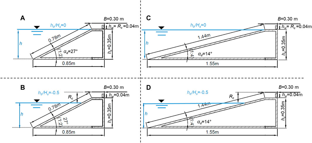
FIGURE 1. Schemes of 4 of the structure configurations and relative geometric parameters tested at the University of Bologna and selected to be reproduced with the numerical code.

TABLE 1

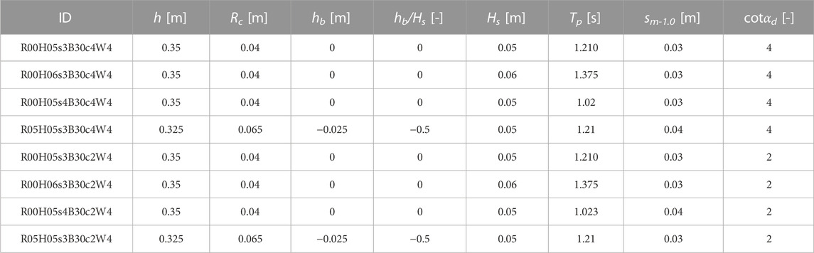
TABLE 1. Main parameters characterizing the eight tests of the validation dataset. B = 0.3 m and h_w = 0.04 m for all the tests. R_c is the structure total freeboard including the crown wall height. H_s and T_p refer to the target values set up in the laboratory.

The small-scale wave flume of the Hydraulic Laboratory of Bologna is 12 m long, 0.5 m wide, and 1.0 m deep, and it is equipped with a piston-type wave maker capable of generating irregular wave series. Both the wave flume and the structure were provided with several instruments to perform the measurements required to assess the hydraulic and structural performance of such structures. The incident and the reflected waves are measured by means of three wave gauges, placed at approximately 1.5∙times the spectral wavelength L_m-1,0 (≈3 m) from the structure toe, i.e., at ≈4.9 m, ≈5.03 m, and ≈5.14 m far from the wave maker. The surface elevations were recorded at a sample frequency of 100 Hz and were elaborated according to the methodology proposed by Zelt and Skjelbreia (1992) to separate the incident from the reflected waves in the wave flume. All the spectral wave parameters T_m-1,0 (wave period), L_m-1,0, s_m-1,0, and ξ_m-1,0 were calculated based on the incident wave spectra. The overtopping water was collected in a calibrated tank, located at the rear side of the structure, to estimate the mean overtopping discharge rate q with a precision of 1∙10^–5 m³/s (Formentin et al., 2019). The pressures acting along the crown wall were measured by means of three transducers (Figure 2), characterized by a sampling frequency of 1 kHz, a range of measurement from 70 mbar to 700 mbar, an accuracy of ±0.04% of the full scale, an external diameter of 25 mm, and an internal diameter of 3 mm. A full HD camera was placed outside the wave flume to the structure side and recorded the wave run-up and the overtopping processes. A recirculation system, composed by a recirculation conduit and a pump (placed in a chamber behind the wave maker), allowed keeping the water level difference within a range of ±4 mm for each test (Formentin et al., 2021a).

FIGURE 2

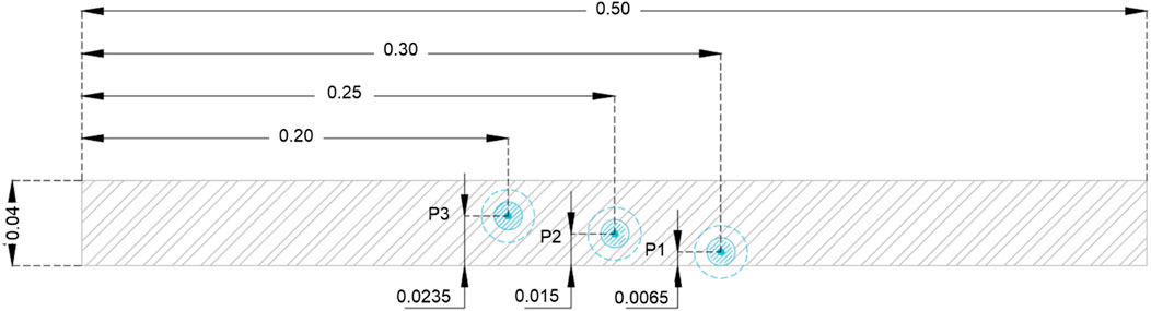
FIGURE 2. Position of the pressure transducers P1, P2 and P3 along the crown wall (hw = 0.04 m) during the laboratory investigation. Front-view cross-section. All the measures are in m.

3.2 Numerical setup and measurements

The numerical domain was built in the OF environment, and it is reproduced in Figure 3. In this figure, the length and the height of the channel are represented along the x-and the z-axis directions, respectively.

FIGURE 3

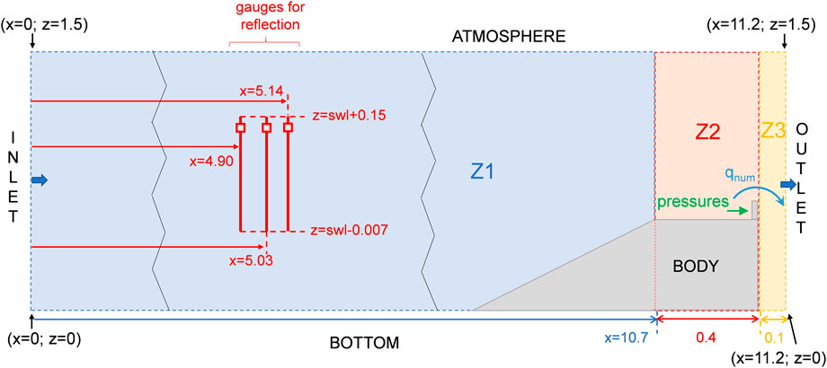
FIGURE 3. Scheme and dimensions of the 2D numerical domain, with reference to the position of the virtual gauges (red) and the quantities measured (overtopping discharge and pressures at the wall). The reference to the three zones of the mesh grid (Z1, Z2 and Z3) and to the domain boundary names is also provided. The “zig-zag” lines indicate where the domain length was cut to fit the Figure in the available space. All the measures are in m.

The numerical wave flume was designed to be 11.2 m long (x) to reproduce exactly the distance between the wave maker downstream edge and the dike inshore edge, which is 11.05 m in the laboratory channel (Formentin et al., 2021a), and an additional area of 0.10 m to realize the outlet relaxation zone for the wave absorption and correctly represent the wave overtopping behind the crown wall. The inlet relaxation zone for the wave generation was set to be 4.5 m long: this length was set up for as much length as possible to optimize the relaxation zone, while keeping a minimum distance between the end of the relaxation area and the dike offshore edge of approximately three times the maximum wavelength measured in the laboratory, L_m-1,0 = 2.24 m. No water was set at the rear side of the structure, as in the laboratory setup.

The height of the domain (z) was set to 1.5 m to provide enough space for air recirculation inside the system: several studies, using the IF package for wave generation by means of the plug-in WF, revealed, indeed, the presence of wiggles in the air–water interface and of spurious velocities in the low-density phase, up to 5–6 times the maximum horizontal velocity of the wave field (Jacobsen, 2012; Larsen et al., 2019). Larsen et al. (2019) demonstrated that this unbalanced behavior is due to the difference between the air and water density. Though Larsen et al. (2019) also demonstrated that such a phenomenon does not influence the wave kinematics, allowing long wave propagation without changing the shape of the wave front, the atmosphere patch was placed ≈20∙H_s (≈1.2 m) above the top of the structure to ensure a better recirculation of air.

The boundary conditions set up for the two solvers WF and CWF at the inlet, bottom, atmospheric, and outlet patches and at the structure (body) are reported in Table 2 and in Figure 3, where the terms follow the syntax of OF. The main variables to be initialized at each boundary are as follows: the VOF (α, in the OF syntax), the dynamic pressure (p_rgh), and the velocity field (U). For the compressible solver, it is necessary to also set up the temperature (T) and the total pressure p. The former was set equal to 300 K (≈27°) and constant for the whole simulation, while for the latter, the boundary conditions “calculated” and “zeroGradient” were, respectively, applied at the four patches of the numerical domain and at the structure.

TABLE 2

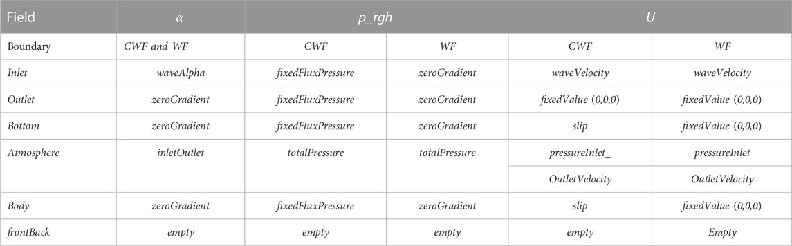
TABLE 2. Boundary conditions for the incompressible (WF) and compressible (CWF) solvers.

For both the WF and CWF solvers, the boundary conditions associated to the frontBack patches—i.e., the side faces of the numerical domain in the (x, z) plane—were set to “empty” because of the 2D nature of the numerical investigations.

The computational domain was discretized through a single hexahedral block mesh, where the origin (x = 0; z = 0) coincided with the bottom-left corner of the numerical domain. The mesh grading was performed both in the x and z directions, in order to obtain refined areas in correspondence of the structure and of the still water level (SWL hereafter), respectively. These refinements aim at improving the representation of the wave development and the resolution of the results in the area of the wave–structure interactions. As shown in Figure 3, the mesh was subdivided into three zones in the x-direction—Z1, Z2, and Z3—whose extension, cell size, and cell numbers are reported in Table 3. In the z-direction, the cell size varied from 0.01 m to 0.002 m from the bottom to the SWL and from 0.002 m to 0.05 m from the SWL to the atmosphere patch. The number of cells in the z-direction is not provided in Table 3 as it varied with the profile of the solid structure. Overall, the total number of cells of the computational domains was 117′182 and 112′762 for the tests at h_b/H_s = 0 in case of c2 and c4, respectively, and 115′518 and 109′516 for h_b/H_s = −0.5. As reported in Table 3, the number of cells per wave height varied between 5 and 25 in the wet area and between 25 and 1 in the air. In the part of the domain included within SWL±1.5H_s, the number of cells per wave was on average 20 and at minimum 18. These numbers are in line with the indications by Chen (2019), who obtained reasonable wave elevation profiles even for a coarser mesh size of six cells per wave height and who suggested anyway to adopt 18 cells per wave height to prevent spurious velocities due to high Courant numbers. Particular evaluation of the mesh size convergence for further applications of the numerical model could consider methods such as the grid convergence index (GCI) (Saghi and Parunov, 2023).

TABLE 3

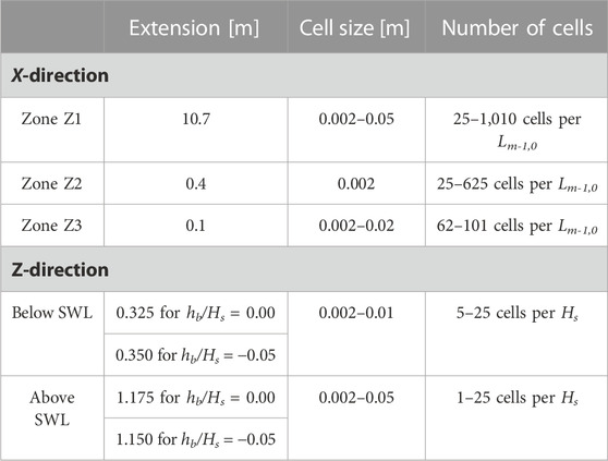
TABLE 3. Extension, cell size, and number of cells in the x (horizontal) and z (vertical) directions of the numerical domain.

The incident wave signals were forced at the inlet boundary by imposing the levels of the free surface elevation measured in the wave flume without the structure and the velocities at the wave paddle that did correspond to the measurements through FFT. Simple linear superposition of the first-order irregular theory implemented in WF for irregular waves was used but considering the amplitude of the ith component, wave number, frequency, and phases resulting from FFT. This element was essential to perform a time-domain comparison between numerical and laboratory models and to specifically compare the shape of wave pressure signals at the walls (Sub-Section 5.2).

The numerical free-surface signals did coincide perfectly in generation, whereas some differences were observed after ≈25–30 s of simulation, principally related to the wave reflection. Both the solvers slightly underestimate some of the laboratory data of H_s (−3% on average) and tend to overestimate the laboratory data of T_p (+16% on average). None of the simulations showed signs of numerical damping. Further comments on this topic are given in Section 4.1.

The computational domain was equipped with three numerical probes to define the surface elevation and so the incident wave. Their location—referenced in Figure 3—corresponds to the same positions as the resistive gauges installed in the wave flume of the laboratory. Another virtual gauge composed by 30 probes was placed at the rear side of the crown wall to calculate the numerical specific overtopping discharges (q_num, m³/(sm)): such quantity was obtained by integrating the horizontal components of the water velocity field, u_x, along the height of the overtopping layer, with a resolution of 0.005 m in the z-direction, see Figure 4. The thickness of the overtopping water layer was isolated by analyzing the values of the VOF (α) field in correspondence of the virtual gauge, step-by-step.

FIGURE 4

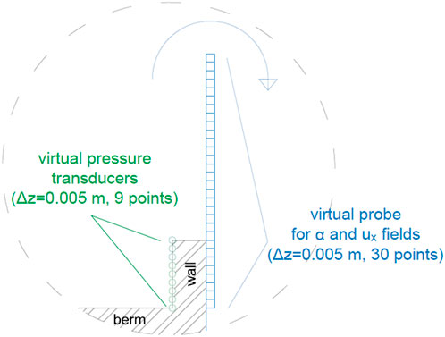
FIGURE 4. Particular of the berm and crown wall in the numerical domain and positions of the pressure transducers and virtual probes for the measurement of the wave pressures and of the wave overtopping discharge, respectively.

The same discretization of 0.005 m was adopted to set up the numerical pressure transducers along the crown wall, leading to nine measuring points (Figure 4). The selected output frequencies to evaluate both the values of q_num and of the wave pressures are, respectively, 20 and 500 Hz. The latter one is high enough to capture the wave impact frequencies, i.e., the frequencies between the maximum and average pressure peaks, which in the laboratory resulted in the range of 140–260 ms. The same frequency of 500 Hz was also adopted to extrapolate the VOF values in correspondence of the pressure transducers to reconstruct the percentages of the air phase Air% during the impact events. This analysis is the subject of ongoing research.

4 Verification of the stability of the compressible solver

This section presents the results of the CWF in terms of hydraulic performance, in order to check its numerical stability and adequacy to represent the wave–structure interaction processes. For this purpose, Sub-Section 4.1 proposes the comparison between numerical and laboratory results of the incident wave heights, peak wave periods, bulk reflection coefficients (K_r), and spectral wave energy associated with the eight tests listed in Table 1. Sub-Section 4.2 focuses on the analysis of the average wave overtopping discharge (q). The values of q were calculated behind the wall, while the values of K_r were estimated in front of the structure.

4.1 Wave generation and reflection

Despite the free-surface values obtained in the numerical channels perfectly coinciding with the laboratory values in generation, there is a slight difference in distribution of the spectral energy associated to the incident and reflected waves. As an example, Figures 5A,B show the spectra of, respectively, the incident and reflected waves, associated to the test R00H05s4B30c4W4. Both the numerical solvers overestimate the peak of the incident wave energy (Figure 5A) and present a shift of the peak wave frequency with respect to the laboratory values. Similarly, the two codes tend to also overestimate the peak of the reflected wave energy (Figure 5B), though in this case the WF code does not show any evident shift of the peak wave frequency, whereas the CWF code still presents a redistribution of the reflected wave energy toward lower frequency values with respect to the laboratory values. Overall, the CWF code presents ≈+25% of reflected wave energy with respect to the WF code and ≈+15% with respect to the laboratory values. Similar results are observed for all the other tests, with the exception of those carried out with emerged structure crest levels. For these tests, the results were exchanged: the WF code presented a higher amount of wave energy in correspondence of low-frequency values, whereas the CWF code did not.

FIGURE 5

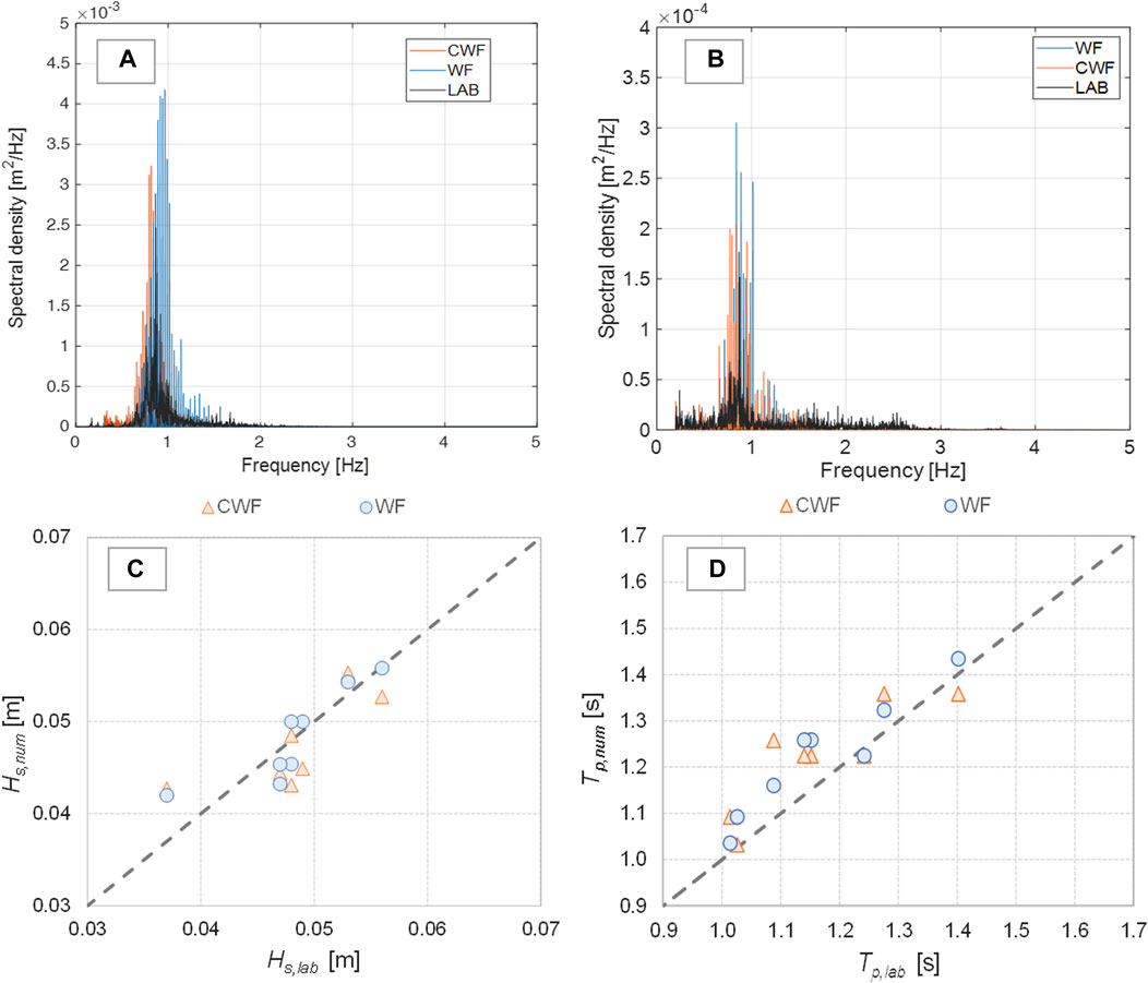
FIGURE 5. Panels (A) and (B): spectra of the incident (A) and reflected (B) waves associated to one example test (R00H05s3G30c4W4). Panels (C) and (D): comparison between the experimental and numerical values of H_s (C) and of T_p (D) obtained with CWF (triangles) and WF (circles).

The evidence of the spectral analysis does reflect into the values of the wave heights and periods measured in the numerical channels. Figures 5C,D, respectively, report the numerical values of H_s and T_p (H_s,num and T_p,num, hereinafter) in comparison to the corresponding experimental data (H_s,lab and T_p,lab) for the eight tests listed in Table 1. From these plots, we can observe that a slight underestimation of the H_s-values performed by the numerical codes occurs together with a slight overestimation of the T_p-values, particularly for CWF. This could be possibly related to effects from fluid compressibility; however, further comprehensive studies should be conducted to address these differences with focus on the fluid interphase interaction and wave propagation considering compressibility.

Finally, based on the qualitative comparison between the numerical (K_r,num) and laboratory (K_r,lab) values of the bulk wave reflection coefficients K_r provided in Figure 6, the two solvers show different results in the case of modest or strong reflection: up to K_r,lab≈0.5, the WF tends to underestimate, while the CWF tends to overestimate the experimental values; for K_r,lab≈0.5, the two codes present almost the same values of K_r,num, which are both very close to experimental values; for K_r,lab>0.6, CWF and WF invert the tendency shown for lower reflection values and, respectively, underestimate and overestimate the K_r,lab-values. On average, the mean relative errors (K_r,num- K_r,lab)/K_r,lab are equal to −8% and +15% for WF and CWF, respectively.

FIGURE 6

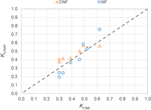
FIGURE 6. Comparison between laboratory (K_r,lab) and numerical (K_r,num) reflection coefficients.

4.2 Wave overtopping discharge

The instantaneous values of q associated to CWF and WF were calculated by integrating the instantaneous values of the cross-shore directed flow velocity (u_x) recorded at the first cell of the numerical domain behind the wall with the corresponding instantaneous overtopping layer thickness. The average values of the numerical overtopping discharge (q_num) were then obtained by time-averaging the instantaneous values of q. Similarly to the procedure adopted for the laboratory measurements, the numerical values of K_r (K_r,num) have been extracted through the separation of the incident and reflected waves (Zelt and Skjelbreia, 1992) from the free-surface elevation time series.

The comparison between the laboratory q_lab and numerical q_num values of q is reported in Figure 7 in terms of dimensionless quantities q/(gH_s³)^0.5, where H_s is the measured wave height. Figure 8 compares the same numerical and laboratory data to the predicting equations of q by EurOtop (2018) in case of smooth, composite structures with crown walls:

$\frac{\mathit{q}}{\sqrt{\mathit{g}{\mathit{H}}_{\mathit{m}\mathbf{0}}^{\mathbf{3}}}}=\frac{\mathbf{0.023}}{\sqrt{\mathit{tan}{\mathit{\alpha }}_{\mathit{d}}}}\bullet {\mathit{\xi }}_{\mathit{m}-\mathbf{1,0}}\bullet \mathit{exp}\left(-{\left(\mathbf{2.7}\bullet \frac{{\mathit{R}}_{\mathit{c}}}{{{\mathit{\xi }}_{\mathit{m}-\mathbf{1,0}}\bullet \mathit{H}}_{\mathit{s}}\bullet {\mathit{\gamma }}_{\mathit{G}\mathit{P}}^{*}}\right)}^{\mathbf{1.3}}\right),{\mathit{\xi }}_{\mathit{m}-\mathbf{1,0}}\le \mathbf{2},(\mathrm{11a})$

$\frac{\mathit{q}}{\sqrt{\mathit{g}{\mathit{H}}_{\mathit{m}\mathbf{0}}^{\mathbf{3}}}}=\mathbf{0.09}\bullet \mathit{exp}\left(-{\left(\mathbf{1.5}\bullet \frac{{\mathit{R}}_{\mathit{c}}}{{\mathit{H}}_{\mathit{s}}\bullet {\mathit{\gamma }}_{\mathit{G}\mathit{P}}^{*}}\right)}^{\mathbf{1.3}}\right),{\mathit{\xi }}_{\mathit{m}-\mathbf{1,0}}>\mathbf{2},(\mathrm{11b})$

where R_c is the structure’s total freeboard including the crown wall height and the reduction factor γ*_GP as derived by Formentin and Zanuttigh (2019) with the genetic programming technique and fitted on the available data (i.e., the database by Van Doorsaler et al., 2015 and the experimental and numerical data by Zanuttigh and Formentin, 2018). This coefficient reads

${\mathit{\gamma }}_{\mathit{G}\mathit{P}}^{*}=\left(\frac{\mathbf{0.93}}{\mathit{tanh}\left(\mathbf{1.5}\bullet {\mathit{\xi }}_{\mathit{m}-\mathbf{1,0}}\right)}\right)-\left(\mathbf{0.30}\bullet \mathit{tanh}\left(\frac{\mathit{B}}{{\mathit{L}}_{\mathit{m}-\mathbf{1,0}}}\right)\right)-\left(\mathbf{0.40}\bullet \mathit{tanh}\left(\frac{{\mathit{h}}_{\mathit{w}}}{{\mathit{R}}_{\mathit{c}}}\right)\right)\bullet -\left(\mathbf{0.15}\bullet {\mathit{\epsilon }}_{\mathit{r}\mathit{a}\mathit{d}}\right),(\mathrm{11c})$

where ε_rad is the angle of the parapet if present on the top of the crown wall. Eq.11a and (11b) are, respectively, valid for breaking and non-breaking waves, where the wave breaking is assumed to occur when ξ_m-1,0 ≤ 2 and is ξ_m-1,0 calculated at the toe of the structures. The two curves representing Eq. 11a and Eq. 11b are plotted as solid lines in Figures 8A,B, respectively, whereas the 90% confidence bands associated to the curves are reported in dashed lines. In the two charts of Figures 8A,B, the ordinates represent the dimensionless data of q divided by different parameters to match the form of Eq. 11A,B, and specifically: q/(gH_s³)^0.5∙(H_s/L_m-1,0∙tgα_d))^0.5 and q/(gH_s³)^0.5, respectively. In Figure 8A, all the tests refer to breaking wave conditions and are associated to the structure slope “c4”, i.e., cotα_d = 4, while in Figure 8B, all the tests represent non-breaking waves and are associated to the slope “c2”, i.e., cotα_d = 2.

FIGURE 7

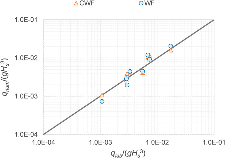
FIGURE 7. Comparison between the laboratory qlab and the numerical qnum average overtopping discharge rates [m²/s]. The continuous line represents the perfect agreement qnum=qlab.

FIGURE 8

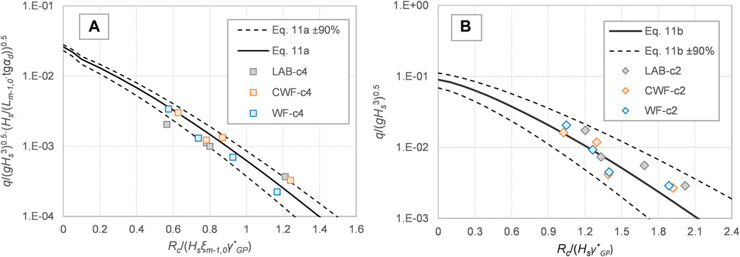
FIGURE 8. Comparison between laboratory and numerical dimensionless data of q (ordinate) and curves representing Eqs. (11a) and (11b) in the charts a and b, respectively.

In both Figure 7 and Figure 8, the q_num values calculated with CWF and WF are displayed in orange and blue colors, respectively. Both the CWF and the WF values of q_num show a good agreement with respect to the laboratory results q_lab (Figure 7), despite the different methodologies used to quantify the average overtopping discharge rates and the differences in the measured values of H_s and T_p (Sub-Section 4.1). Statistical errors have been computed to quantify the reliability of the two solvers. Specifically, the following indexes have been calculated and reported in Table 4: the relative errors (q_num-q_lab)/q_lab, the root mean square error (rmse), and the coefficient of correlation R². Figure 7 shows that both the WF and the CWF data are very similarly distributed around the line representing the perfect agreement, showing approximately the same level of agreement with the experimental measurements and the absence of bias (relative errors 9% and 16%, rmse = 2.35∙10⁻³ m³/(s∙m) and 2.13∙10⁻³ m³/(s∙m), respectively). Based on these results, it could be concluded that the slight underestimation of the H_s-values performed by the numerical codes (Sub-Section 4.1; Figure 5C) is balanced by the slight overestimation of the T_p-values (Figure 5D), resulting in an overall good representation of q.

TABLE 4

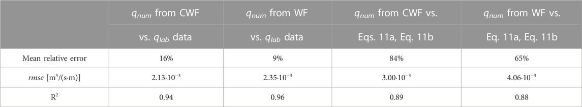
TABLE 4. Performance indexes of the agreement between laboratory and numerical data of q and numerical data of q and Eq. 11a, Eq. 11b.

The data of q calculated with the two solvers also fit similarly the EurOtop equations, as indicated by the performance indexes and by the charts of Figure 8. All the data fall within the 90% confidence bands associated to the formula (dashed lines in Figure 8), though in case of breaking waves (Figure 8A), the q-values resulting from the WF code are slightly but systematically below those given in the formula. Overall, the predictions of q obtained with CWF are at least as reliable as the ones derived with the existing solver.

5 Verification of wave pressures and forces

This section analyzes the results of the numerical simulations in terms of wave loads at the crown walls to verify the presence and relevance of the air entrainment and the capability of the CWF code to represent it. Sub-Section 5.1 presents a literature overview related to the wave impact dynamics and some considerations on the role of the air entrainment. Sub-Section 5.2 discusses, from a qualitative point of view, the reliability of the CWF solver to reproduce the different types of wave impacts observed during the laboratory campaign and illustrated in the literature review. Sub-Section 5.3 focuses on the statistical analysis of the pressure values. Finally, Sub-Section 5.4 presents and compares the values of the wave forces resulting from the simulations with WF and CWF and from the laboratory measurements.

5.1 Literature overview of the impact classification methods

Both the magnitude and the shape of the signal of the impact pressures are first determined by the position of the breaking point and second by the breaker type (Chan and Melville, 1988; Witte, 1988). A common result of the physical observations is the influence of the water–air mixtures on the shape and magnitude of the pressure signals associated to the wave impacts (see for a review Bullock et al., 2007). The pressure over time presents an impulsive component (maximum value), i.e., a very short duration shock pressure, followed by a quasi-hydrostatic component characterized by a lower, almost constant, value. Bagnold (1939) was the first to directly link the shock pressure to the presence of the air pocket, which is subjected to a compression/expansion process during the wave–structure interaction. This dynamic produces oscillations of the pressure signal, which are damped afterward due to the leakage of the trapped air and the disintegration of the air pocket into a bubbly flow (Bullock et al., 2012). This phenomenon was observed during small- and large-scale experimental campaigns (Schimdt et al., 1992; Hattori et al., 1994; Obhrai et al., 2004; Bullock et al., 2007; Formentin et al., 2021a). Several studies showed that the presence of the air pockets tends to decrease the magnitude of the peak pressures (Plumerault et al., 2012a), while Obhrai et al. (2004) noticed that the spatial extent and the duration of the high-pressure event increases with the air pockets, leading to larger forces against the wall. Furthermore, a series of statistical analysis of the wave load distributions (Schmidt et al., 1992; Hattori et al., 1994) highlighted that high-impact pressures were also registered in case of breakers including air pockets.

By linking the breaking point and the air content, Oumeraci et al. (1993) defined a classification of the wave impacts based on four breaker types: 1) slighting breaking waves, characterized by a turbulent, bore breaker generating the smallest impact pressures and forces; 2) well-developed plunging breakers, with large air cushions, generating relatively high impact loads; 3) plunging breakers with small air cushions, determining the most striking impact loads; 4) upward deflected breakers with no air entrapped, determined by quasi-standing waves and generating no sharp pressure peaks nor huge impact loads. The distance between the breaking point and the wall decreases from breaker types (1) to (4) mentioned previously.

Following this classification, Bullock et al. (2007) performed a specific laboratory campaign to introduce a more detailed classification of the impacts focusing on the air content. Combining visual observations with signal processing, this study identified two levels of aeration, i.e., the low- and the high-aerated impacts. Both broadly fall within the category of impact loads by Oumeraci et al. (1993), and the two impacts mainly differ in terms of the amount and the type of the air entrapped and in the characteristic trace generated in the pressure signal. The low-aeration impacts can be associated to a pressure “church spire” shape, and the aeration content is due to the presence of bubbles and/or entrapment of small air pockets. For the high-aeration impacts, the pressure trace is characterized by strong oscillations due to appreciable-sized air pockets, subjected to expansion/compression phases. Eventually, Bullock et al. (2007) classified the impacts as broken when the waves break before reaching the wall, involving significant quantities of air and relatively low-pressure spikes. Although this categorization could experience a degree of subjectivity due to the complexity of the phenomenon, it is possible to assert that the strong oscillations in the pressure trace are mostly associated to impacts characterized by significant air content. In this case of high-aerated signals, sub-atmospheric peaks, taking place after the main impact, were also observed (Oumeraci et al., 1999; Bullock et al., 2007; NAUE, 2012; Formentin et al., 2021a).

In summary, the literature proposes the following three main classification methods to describe the different wave impacts that may occur:

• The nature of wave impact (impact load, slightly breaking wave, and broken wave), developed by Oumeraci et al. (1993).

• The nature of the wave breaking (surging, plunging, and broken), based on the breaker parameter ξ_m-1,0.

• The air content associated to the wave impact (high-aeration, low-aeration, and broken), following Bullock et al. (2007).

These methods are summarized and matched together in Table 5.

TABLE 5

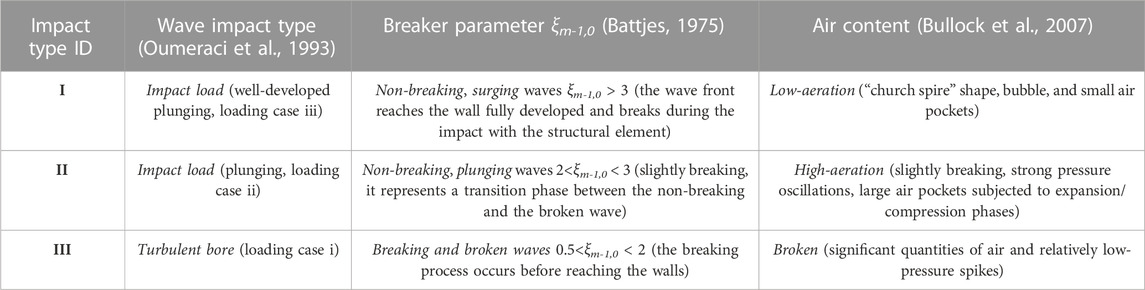
TABLE 5. Classification and description of the tested wave conditions according to the breaker parameter, the type of the wave impact, and the associated air content.

Figure 9 proposes a reference example to visualize the characteristic pressure trace associated to the different impact types recalled in Table 5. Indeed, in this plot—representing 4 s of the time signal of the wave pressure recorded at the transducer P2 during one of the laboratory experiments—all the three impacts are visible: a broken wave (impact type III, 0.5<ξ_m-1,0 < 2), a surging wave (impact type I, ξ_m-1,0 > 3), and a plunging wave (impact type II, 2<ξ_m-1,0 < 3), in time-sequential order. In agreement with Oumeraci et al. (1993) and Bullock et al. (2007), each wave impact shows two pressure peaks: the first peak leads to the maximum pressure value (p_max, hereinafter), and it is followed by a trace of different duration and various oscillation frequency and amplitude, based on the impact type; the second, lower peak comes after the pressure oscillations and represents the quasi-hydrostatic pressure value characterizing the wave impact (p_h,q, hereinafter).

FIGURE 9

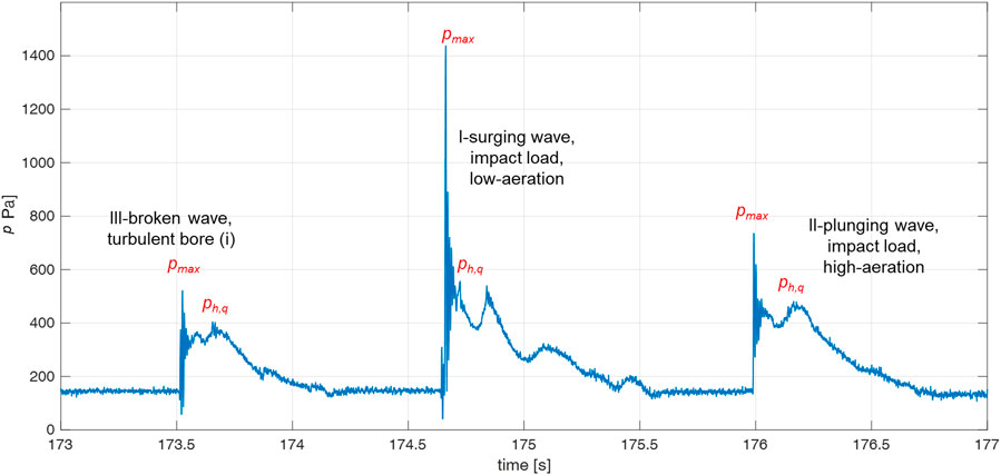
FIGURE 9. Example of pressure signals over time extracted from one laboratory record showing three different impact types: broken, surging, and plunging.

According to the PROVERBS project (Oumeraci et al., 1999), a specific range of values of the ratio p_max/p_h,q is associated to each breaker type: 1<p_max/p_h,q<2.5 for the plunging waves (II), p_max/p_h,q>2.5 for the surging waves (I), and p_max/p_h,q≈1 for the broken waves (III).

5.2 Characterization of the wave pressure signals over time

The laboratory and numerical tests (Sub-sections 3.1 and 3.2, respectively) were analyzed to characterize the resulting pressure signals in the literature framework. To this purpose, it was necessary to individuate the single-wave impacts from the pressure time series and to identify the p_max and p_h,q-values of each impact event.

The number of the wave impacts N_imp was calculated for each test and at each pressure transducer by adopting the methodology described in Formentin et al. (2021a). In brief, this methodology consists of a MATLAB procedure that finds the local maxima in the pressure signals based on the definition of a minimum threshold value of p to separate the real impacts from oscillations or noise in the signal. In Formentin et al. (2021a), such threshold was set equal to p₁₀₀/3 Pa, where p₁₀₀ was estimated as the average pressure impact value of the highest 1/100th overtopping waves. Each impact event is timely circumscribed by two consecutive down-crossing of the threshold p-value. Once defined an impact event, p_max was identified as the local maximum of the pressure trace included in the time-limits of the impact. p_h,q was calculated by adopting the second step of the procedure described in detail in Formentin et al. (2021a). Such a procedure is based on the definition of the minimum and maximum time delay that may occur between the maximum and the quasi-hydrostatic peaks. (Further details are given in Formentin et al., 2021a). Following this methodology, the values of p_max and p_h,q were calculated for each wave impact recorded at each pressure transducer of each laboratory and numerical test.

In the illustration of pressure signals within Figure 10, the threshold values of p are represented by orange triangles, whereas p_max and p_h,q are, respectively, represented as violet circles and yellow crosses.

FIGURE 10

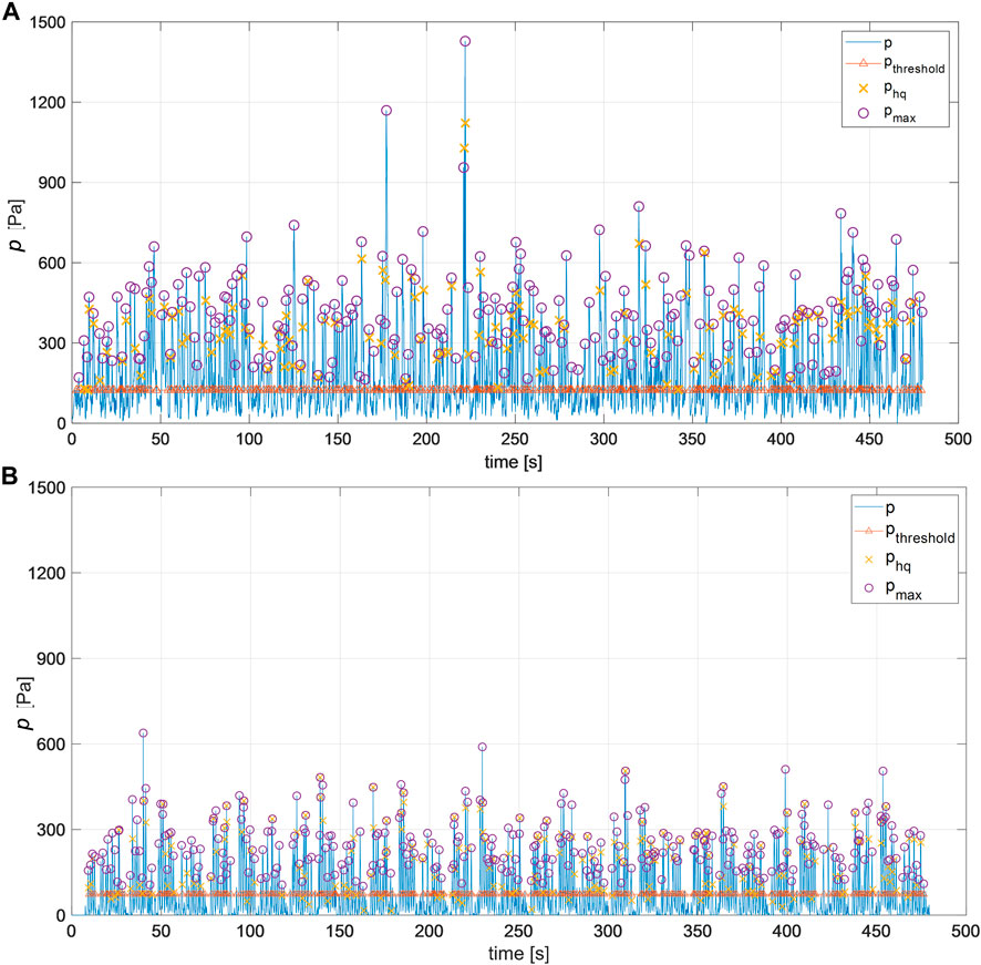
FIGURE 10. Comparison of the same pressure signal over time (0–500 s) resulting from the simulation of the test R00H06s3G30c2W4 with the CWF panel (A) and WF panel (B) solvers.

The results of the analyses of the p_max and p_h,q indicate that

• The laboratory tests involved all the three impact types summarized in Figure 9, with the following average occurrence rates: surging (I) 3%–8%, plunging (II) 80%–85%, and broken (III) 6%–16%.

• The same rates were approximately found for all the experiments reproduced with the numerical code CWF.

• Significant lower numbers of surging (I) waves were observed for the simulations run with the WF code (0.05%–0.5%), and consequently, larger percentages of plunging (II, ≈85%) and broken (III, ≈15%) cases were found.

An empirical explanation to the very low number of surging waves associated to the WF simulations can be found in Figure 10, which compares the two wave pressure signals recorded for the example test R00H05s3G30c2W4 reproduced with the CWF (panel a) and the WF (panel b) solvers. The signal in Figure 10B presents, indeed, a significant lower variability, being characterized by a standard deviation of σ = 121 Pa, whereas σ = 146 and 151 Pa for the CWF and the corresponding laboratory test, respectively. Furthermore, the WF code provides lower pressure values on average (the mean values of p are 126, 186, and 185 Pa for WF, CWF, and laboratory test, respectively) and lower peaks, which are approximately 500 Pa, where the occurrence of conditions with p_max/p_h,q>2.5 is extremely rare.

The WF code also prompted a limited number of p_max and p_h,q-values (precisely 294, represented, respectively, by violet circles and yellow crosses in Figure 10), with respect to the CWF code (372) and the laboratory values (351).

Focusing on the details of the pressure signals, Figure 11 proposes, as example, the time–pressure trace associated to the first impact event recorded in the laboratory (gray) and by the CWF (orange) and WF (blue) solvers for the test R00H05s3G30c4W4. According to Oumeraci et al. (1993); Bullock et al. (2007), the event recorded in the laboratory corresponds to a high-aeration impact of type II, being the ratio p_max/p_h,q≈2.5, considering the presence of a negative pressure peak of −200 Pa immediately after the maximum and of the subsequent pressure oscillations, and being the duration of the impact of ≈300 ms.

FIGURE 11

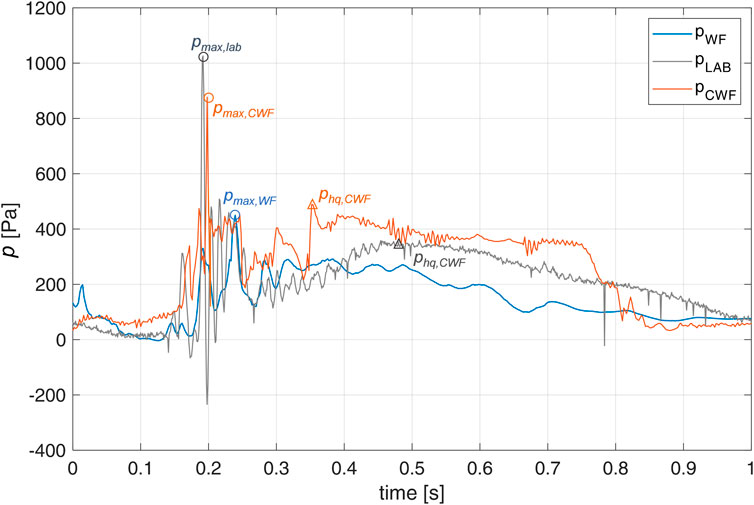
FIGURE 11. Comparison of the first impact event recorded at the transducer P2 during the run of the test R00H05s3G30c4W4 in the LAB (grey) and with the WF (blue) and CWF (orange) solvers.

Figure 11 shows that the signal associated to WF hardly presents the typical “church spire” trace expected from the literature and found indeed in the laboratory and CWF signals. The signal obtained with the WF appears smoothed and flattened, missing and severely underestimating the pressure peak of p_max≈1,020 Pa observed in the laboratory at approximately 0.2 s. The WF code also does not capture the oscillations subsequent to the maximum and corresponding to the expansion/compression phases associated to a high-aeration impact. On the contrary, the CWF gives a good estimation of the peak, with p_max≈870 Pa, and it also provides a more similar representation of the pressure trace subsequent to the maximum, reproducing accurately the “flat” part of the “church spire”.

5.3 Statistical analysis and vertical distribution of the wave pressures

The instantaneous p-values measured at the several pressure transducers—and in particular in correspondence of P1, P2, and P3—were treated as stochastic values to extract the following statistics over time: maximum, mean, and median (p_max, p_mean, and p_median) and the quantile 250 (p₂₅₀). Similar to p₁₀₀, this quantile was estimated as the average pressure of the highest N_ow/250 impact events, where N_ow is the number of waves overtopping the berm. The statistics were calculated at each pressure transducer for each of the tests presented in Table 1, performed in the laboratory simulated with the numerical codes. For the experimental tests, the statistics are, therefore, available in correspondence of P1, P2, and P3 only, while for the numerical tests, the statistics were calculated in correspondence of the nine virtual gauges (Figure 4), allowing a more complete and extended vertical profile of the wave pressures at the walls.

Following the common literature approach, which identifies p₂₅₀–or the wave force F₂₅₀—as an estimator of the extreme loads acting on the walls (Goda, 1985; Van Doorslaer et al., 2017) and as an estimator of the quasi-hydrostatic pressures p_h,q (Cuomo et al., 2010b), the analyses of the vertical profiles of the wave pressures are here presented in terms of p₂₅₀.

Figure 12 illustrates the vertical profiles of the p₂₅₀-values obtained from the processing of the laboratory and numerical data for the following four tests: R00H05s3G30c2W4, R05H05s3G30c2W4, R00H05s3G30c4W4, and R05H05s3G30c4W4, charted in the panels (a), (b), (c), and (d), respectively. The four tests differ in terms of the slope (c2 and c4) and the berm emergence (h_b/H_s = 0 and h_b/H_s = −0.5), and they all present H_s = 0.05 and s_m-1,0 = 0.03. The results obtained for the remaining four tests listed in Table 1, concerning different H_s- and s_m-1,0-values, are not shown for brevity, as the wave steepness and the wave height play a pure scale effect on the profiles.

FIGURE 12

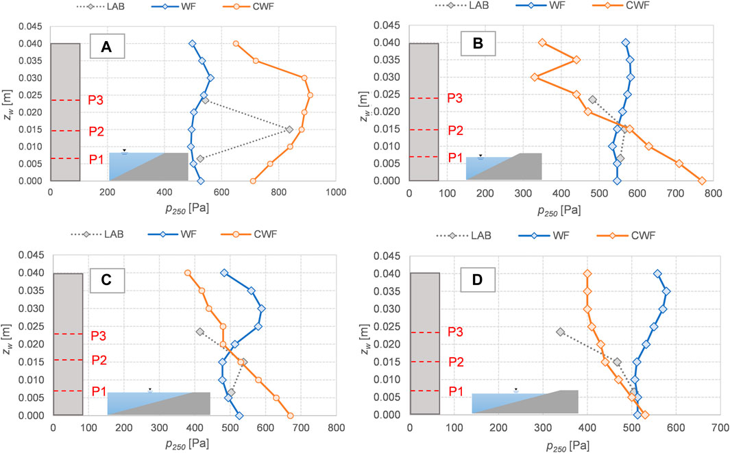
FIGURE 12. Vertical profiles of p250 calculated for four different tests run in the LAB (grey), with the WF (blue) and the CWF (orange) solvers. (A): test at cot(αd) = 2 and hb/Hs = 0; (B): test at cot(αd) = 2 and hb/Hs = −0.5; (C): test at cot(αd) = 4 and hb/Hs = 0; (D): test at cot(αd) = 4 and hb/Hs = −0.5. For all the tests: Hs = 0.05 m, sm−1,0 = 0.03, B = 0.3 m, hw = 0.04 m.

For all the tests, the experimental and numerical values of p₂₅₀ obtained with the CWF code at the pressure transducer P2 are basically identical. As for the other pressure transducers, the CWF code shows shapes of pressure profiles more similar to the experimental data with respect to WF for all the tests of panels b, c, and d. In panel a, both the solvers WF and CWF do not seem to capture the triangular shape of the pressure profile registered in the laboratory for this test. Here, the CWF code significantly overestimates the p₂₅₀-values at P1 and P3, showing a completely different profile with respect to the laboratory. In particular, CWF shows wave pressures almost constant along the vertical axis up to z_w = 0.025 m, while in the laboratory, the pressures almost reduce by half from P2 to P3. Incidentally, WF provides a good representation of p₂₅₀-values at P1 and P3 for the test in panel a, but it severely underestimates p₂₅₀ at P2 and shows regular, almost constant profiles of the wave pressures along the vertical axis here and for all the other values.

Overall, the analyses of the pressure signals in the time domain (Sub-section 5.2) and the statistical analysis of the extreme pressure values (this section) indicate that the WF cannot capture the peaks of the wave pressures and cannot adequately reproduce the shape of the pressure signals and profiles. On the contrary, the CWF always gives a cautious estimation of the extreme p-values and gives a more realistic representation of signals and profiles.

5.4 Design wave loads

The instantaneous p-values resulting from the laboratory and from the CWF and the WF solvers were integrated along the wall height to obtain the instantaneous hydrodynamic forces, F. The numerical and experimental F-values are derived, therefore, from integrating, respectively, the nine and the three pressure gauges, with the space-resolution of the p-values playing a significant role in the estimation of the F-values. The same statistics for the p-values were calculated for the F-values, and, in particular, the quantiles F₂₅₀, which are adopted to check the capability of the new and existing codes to reproduce the extreme wave loads in comparison to laboratory data and literature formula.

The experimental and the numerical dimensionless values F₂₅₀/ρgR_c² are hereinafter compared to the following reference formula by Van Doorslaer et al. (2017):

$\frac{{\mathit{F}}_{\mathbf{250}}}{\mathit{\rho }\mathit{g}{\mathit{R}}_{\mathit{c}}^{\mathbf{2}}}=\mathbf{7.8}\bullet \mathit{exp}\left(\mathit{b}\bullet \frac{{\mathit{R}}_{\mathit{c}}}{{\mathit{H}}_{\mathit{s}}}\right),(12)$

where g is the acceleration of gravity and R_c is the structure’s total freeboard including the wall height (R_c = h_w-h_b, Figure 1). This formula was developed based on three different experimental datasets, including tests of smooth dikes with sloping promenades and crown walls at different scale. For the present study, the value of b = −2.02 was chosen as for small-scale tests.

All the wave force values were made dimensionless with ρgR_c² by assuming the water default value of ρ = 1,000 kg/m³. Indeed, for the experimental tests and for the simulations run with the WF code, which disregards the fluid compressibility, it is impossible in practice to calculate the actual density of the fluid mixture air/water. For the CWF code, the mixture density value ρ is available for each cell of the numerical domain and at each time step. However, the instantaneous ρ-value depends also on the degree of wetting of the cells, which is unknown. Since the numerical pressure gauges at the wall are above the water free-surface for most of the simulation time, it is impossible to establish whether a cell value of ρ resulting <1,000 kg/m³ is due to a partial wetting of the cell and/or to an actual compression of the air density. In conclusion, to bypass this issue and to be consistent with the experimental data and the WF simulations, ρ was considered equal to 1,000 kg/m³ also for the CWF tests.

The comparison between data and Eq. 12 is qualitatively provided in Figure 13, where the formula is represented as a continuous line and referenced as “VD.” The agreement among the numerical results, the experimental data, and Eq. 12 is remarkable, with the relative differences (F_250,CWF-F_250,Eq.13)/F_250,Eq.13 = 9%, (F_250,WF-F_250,Eq.13)/F_250,Eq.13 = −8%, and (F_250,LAB-F_250,Eq.13)/F_250,Eq.13 = 10%, on average, where F_250,Eq.13, F_250,CWF, F_250,WF, and F_250,LAB are the F₂₅₀-values resulting from Eq. (13), the CWF code, the WF code, and the laboratory test, respectively. Half of the results of the CWF code fall instead above the curve. The laboratory data present a little greater scatter, which could be probably related to the higher level of uncertainty associated to the measurements. Overall, all the points are close to each other and do not show any evident bias.

FIGURE 13

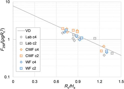
FIGURE 13. Comparison between the laboratory and the numerical (CWF and WF) statistical dimensionless values of F₂₅₀/ρgR_c² (Eq. 12, “VD”).

6 Conclusion

This paper presents the results of the numerical simulations for wave overtopping and wave impacts at crown walls obtained with the suite IsoCompressibleWaveFoam, CWF, developed in the openFOAM environment (Jasak et al., 2007) and consisting in the combination of the existing library waves2Foam (Jacobsen et al., 2012) with the native compressibleInterFoam. CWF is capable of solving two compressible, isothermal, immiscible fluids using a VOF (volume of fluid) phase-fraction approach to capture the interface between the two fluids. CWF was applied for the first time to simulate irregular wave series of at least 400–500 waves, in order to perform a statistical analysis of the hydraulic and structural performance of coastal defenses—accounting for the effects of the air entrainment and compressibility.

Specifically, the CWF suite was applied to reproduce a subset of eight experimental tests recently performed at the Hydraulic Laboratory of the University of Bologna (Formentin et al., 2021a). The tested cases involved a variety of structural configurations under both breaking and non-breaking wave conditions. The run of the eight simulations, which lasted 480 s each, did not show any problem related to the numerical instability and required a reasonable computational effort (a few weeks for each simulation) for a standard work-station PC. The turbulence closure models were not included to save computational time. The same eight tests were simulated also with the incompressible suite waves2Foam (WF), and the results obtained from the two codes were compared to each other and to the measurements from the physical tests and literature formulae.

Despite that turbulence plays a role in the wave breaking and wave transformation before impacting the wall, the results of the numerical simulations in terms of wave overtopping seem not to be significantly affected by the absence of the turbulence model. The values of the wave overtopping discharge q obtained with CWF show, indeed, the same accuracy of WF when compared to the experiments and to the literature formulae (relative errors 0.09 and 0.16, rmse = 2.35∙10⁻³ m³/(s∙m) and 2.13∙10⁻³ m³/(s∙m) for WF and CWF, respectively).

A different representation of the wave reflection was instead observed. CWF presented a redistribution of the reflected wave energy in correspondence with low-frequency values, which led anyway to values of K_r very similar to those obtained with the WF code and to the laboratory data. Calculations based on face fluxes in consistency of numerical volume fluxes could enhance the results of wave overtopping instead of considering average velocities and alpha field thickness as herein presented.

The capability of the CWF solver to represent the different breaker types observed during the experimental campaign, i.e., surging, plunging, and broken waves, and the consequent different wave impacts at the walls, was investigated in comparison to the incompressible suite WF. Overall, the analyses of the pressure signals in the time domain demonstrated that the compressible suite registered approximately the same occurrence rates of the different breakers observed in the laboratory, in line with the existing literature available for larger-scale tests (Oumeraci et al., 1999; Bullock et al., 2007). The WF solver instead significantly underestimated the numbers of surging waves, which are responsible for the most severe wave impacts. Furthermore, the CWF suite reproduced faithfully the shape, the variability, and the peaks of the time–pressure signals recorded in the laboratory, overcoming the limits of the incompressible solver WF, which provided unrealistic, flat signals, characterized by lower pressure values on average and lower peaks.

Similarly, the statistical analysis of the wave pressures suggested that CWF gives a more realistic and a more cautious estimation of the vertical profiles of the p₂₅₀-values along the crown walls for all the tests. On the contrary, the WF revealed to be inadequate to capture the peaks in the pressure profiles, providing almost uniform distribution of the p₂₅₀-values along the vertical.

The design wave forces F₂₅₀—which were calculated from the integration of the p₂₅₀-values along the crown wall height—present a similar agreement with the literature formula by Van Doorslaer et al. (2017), giving average errors of 9% and −8% for the CWF and the WF codes, respectively. The F₂₅₀ data resulting from the CWF and the WF codes are, respectively, slightly underestimated and overestimated by the theoretical trend.

In conclusion, based on the analyses carried out, the compressible solver CWF demonstrated to be at least as stable and as reliable as the incompressible solver WF to simulate hundreds of irregular waves and to reliably reproduce the wave–structure interaction processes for both slightly breaking and fully broken waves striking against a composite, smooth breakwater with a crown wall, under the hypothesis of isothermal conditions. When applied to represent the wave impact processes at the walls—where the role of the air entrainment becomes relevant—CWF outperformed the incompressible suite, reproducing realistically and accurately the pressure signals and values.

The introduction of the turbulence closure model, the application to larger-scale physical tests where even more relevant effects of the air entrainment are expected, and the application to a wider range of structure types represent the next steps to be performed. Further application of the CWF solver is indeed under way to test the compressible suite against a porous breakwater at prototype scale subjected to 3D overtopping waves, to investigate the potentialities of the new developed solver in case of permeable structures, and check possible scale effects.

Data availability statement

The raw data supporting the conclusion of this article will be made available by the authors, without undue reservation.

Author contributions

Conceptualization, BZ, SMF, and JCAH; formal analysis, SMF, GP, and JCAH; investigation, GP and SMF; data curation, GP and SMF; writing—original draft preparation, GP, SMF, and BZ; writing—review and editing, SMF, BZ, and JCAH; supervision, BZ and JCAH. All authors have read and agreed to the published version of the manuscript.

Conflict of interest

The authors declare that the research was conducted in the absence of any commercial or financial relationships that could be construed as a potential conflict of interest.

Publisher’s note

All claims expressed in this article are solely those of the authors and do not necessarily represent those of their affiliated organizations, or those of the publisher, the editors, and the reviewers. Any product that may be evaluated in this article, or claim that may be made by its manufacturer, is not guaranteed or endorsed by the publisher.

References

Aleixo, R., Soares-Frazão, S., and Zech, Y. (2018). Statistical analysis methods for transient flows–the dam-break case. J. Hydraul. Res. 57, 688–701. doi:10.1080/00221686.2018.1516700

CrossRef Full Text | Google Scholar

Altomare, C., Gironella, X., and Crespo, A. J. C. (2021). Simulation of random wave overtopping by a WCSPH model. Appl. Ocean Res. 116, 102888. doi:10.1016/j.apor.2021.102888

CrossRef Full Text | Google Scholar

Bagnold, R. A. (1939). Interim report on wave-pressure research. J. Inst. Civ. Eng. 12, 202–226. doi:10.1680/ijoti.1939.14539

CrossRef Full Text | Google Scholar

Battjes, J. A. (1975). Surf similarity. Coast. Eng., 466–480. doi:10.1061/9780872621138.029

CrossRef Full Text | Google Scholar

Berberović, E., van Hinsberg, N. P., Jakirlić, S., Roisman, I. V., and Tropea, C. (2009). Drop impact onto a liquid layer of finite thickness: dynamics of the cavity evolution. Phys. Rev. E 79 (3), 036306. doi:10.1103/PhysRevE.79.036306

CrossRef Full Text | Google Scholar

Booshi, S., and Ketabdari, M. J. (2021). Modeling of solitary wave interaction with emerged porous breakwater using PLIC-VOF method. Ocean. Eng. 241, 110041. doi:10.1016/j.oceaneng.2021.110041

CrossRef Full Text | Google Scholar

Borsboom, M., and Jacobsen, N. (2021). A generating-absorbing boundary condition for dispersive waves. Numer. methods Fluids 93, 2443–2467. doi:10.1002/fld.4982

CrossRef Full Text | Google Scholar

Brackbill, J. U., Kothe, D. B., and Zemach, C. (1992). A Continuum method for modeling surface tension. J. Comput. Phys. 100 (2), 335–354. doi:10.1016/0021-9991(92)90240-y

CrossRef Full Text | Google Scholar

Bredmose, H., Bullock, G., and Hogg, A. (2015). Violent breaking wave impacts. Part 3: effects of scale and aeration. J. Fluid Mech. 765, 82–113. doi:10.1017/jfm.2014.692

CrossRef Full Text | Google Scholar

Bredmose, H., Peregrine, D., and Bullock, G. (2009). Violent breaking wave impacts. Part 2: modelling the effect of air. J. Fluid Mech. 641 (1), 389–430. doi:10.1017/S0022112009991571

CrossRef Full Text | Google Scholar

Bullock, G. N., Obhrai, C., Peregrine, D. H., and Bredmose, H. (2007). Violent breaking wave impacts. Part 1: results from large – scale regular wave tests on vertical and sloping walls. Coast. Eng. 54 (8), 602–617. doi:10.1016/j.coastaleng.2006.12.002

CrossRef Full Text | Google Scholar

Chan, E. S., and Melville, W. K. (1988). Deep-water plunging pressures on a vertical plane wall London, England: Royal Society of London, 95–131.

Google Scholar

Chen, H. (2019). On the application of OpenFoam^® in gravity water wave generation and wave-structure interaction. J. Ship Res. 63 (02), 130–142. doi:10.5957/JOSR.08180041

CrossRef Full Text | Google Scholar

Chenari, B., Saadatian, S. S., and Ferreira, A. D. (2015). Numerical modelling of regular waves propagation and breaking using waves2foam. J. Clean Energy Technol. 3 (4), 276–281. doi:10.7763/JOCET.2015.V3.208

CrossRef Full Text | Google Scholar

Choi, Y.-M., Kim, J. K., Bouscasse, B., Seng, S., Gentaz, L., and Ferrant, P. (2020). Performance of different techniques of generation and absorption of free-surface waves in Computational Fluid Dynamics. Ocean. Eng. 214, 107575. doi:10.1016/j.oceaneng.2020.107575

CrossRef Full Text | Google Scholar

Conde, J. M. P. (2019). Comparison of different methods for generation and absorption of water waves. Rev. Eng. Térmica 18 (1), 71–77. doi:10.5380/reterm.v18i1.67053

CrossRef Full Text | Google Scholar

Crespo, A. J. C., Domínguez, J. M., Rogers, B. D., Gómez-Gesteira, M., Longshawb, S., Canelas, R., et al. (2015). DualSPHysics: open-source parallel CFD solver based on smoothed particle hydrodynamics (SPH). Comput. Phys. Commun. 187, 204–216. doi:10.1016/j.cpc.2014.10.004

CrossRef Full Text | Google Scholar

Cuomo, G., Allsop, W., Bruce, T., and Pearson, J. (2010b). Breaking wave loads at vertical seawalls and breakwaters. Coast. Eng. 57 (4), 424–439. doi:10.1016/j.coastaleng.2009.11.005

CrossRef Full Text | Google Scholar

Cuomo, G., Allsop, W., and Takahashi, S. (2010a). Scaling wave impact pressures on vertical walls. Coast. Eng. 57, 604–609. doi:10.1016/j.coastaleng.2010.01.004

CrossRef Full Text | Google Scholar

Damiàn, S. M. (2013). An extended mixture model for the simultaneous treatment of short and long scale interfaces. Ph.D. thesis. Santa Fe, Argentina: Universidad Nacional del Litoral.

Google Scholar

El Safti, H., and Oumeraci, H. (2013). “Modelling sand foundation behaviour underneath caisson breakwaters subject to breaking wave impact,” in Proceedings of the 32nd International Conference on Ocean, Offshore and Arctic Engineering, Nantes, France, June, 2013. doi:10.1115/OMAE2013-10281

CrossRef Full Text | Google Scholar

Engsig-Karup, A. P. (2006). Unstructured nodal DG-FEM solution of high-order Boussinesq-type equations. Ph.D. thesis. Denmark, Europe: Technical University of Denmark.

Google Scholar

EurOtop, (2018). Manual on wave overtopping of sea defences and related structures. An overtopping manual largely based on European research, but for worldwide application. www.overtopping-manual.com.

Google Scholar

Formentin, S. M., Gaeta, M. G., De Vecchis, R., Guerrero, M., and Zanuttigh, B. (2021b). Image-clustering analysis of the wave-structure interaction processes under breaking and non-breaking waves. Phys. Fluids 33, 105121. doi:10.1063/5.0065019

CrossRef Full Text | Google Scholar

Formentin, S. M., Gaeta, M. G., Palma, G., Zanuttigh, B., and Guerrero, M. (2019). Flow depths and velocities across a smooth dike crest. Water 11 (10), 2197. doi:10.3390/w11102197

CrossRef Full Text | Google Scholar

Formentin, S. M., Palma, G., and Zanuttigh, B. (2021a). Integrated assessment of the hydraulic and structural performance of crown walls on top of smooth berms. Coast. Eng. 168, 103951. doi:10.1016/j.coastaleng.2021.103951

CrossRef Full Text | Google Scholar

Formentin, S. M., and Zanuttigh, B. (2019). A Genetic Programming based formula for wave overtopping by crown walls and bullnoses. Coast. Eng. 152, 103529. doi:10.1016/j.coastaleng.2019.103529

CrossRef Full Text | Google Scholar

Goda, Y. (1985). Random seas and design of maritime structures. Tokyo, Japan: University of Tokyo, 433.

Google Scholar

Gullbrand, J., and Katopodes Chow, F. (2003). The effect of numerical errors and turbulence models in large-eddy simulations of channel flow, with and without explicit filtering. J. Fluid Mech. 495 (495), 323–341. doi:10.1017/S0022112003006268

CrossRef Full Text | Google Scholar

Hattori, M., Arami, A., and Yui, T. (1994). Wave impact pressure on vertical walls under breaking waves of various types. Coast. Eng. 22, 79–114. doi:10.1016/0378-3839(94)90049-3

CrossRef Full Text | Google Scholar

Hernandez, J., Lopez, J., Gomez, P., Zanzi, C., and Faura, F. (2008). A new volume of fluid method in three dimensions-part I: multidimensional advection method with face-matched flux polyhedra. Int. J. Numer. Methods Fluids 58 (8), 897–921. doi:10.1002/fld.1776

CrossRef Full Text | Google Scholar

Higuera, P., Lara, J. L., and Losada, I. J. (2013a). Realistic wave generation and active wave absorption for Navier–Stokes models: application to openFOAM. Coast. Eng. 71, 102–118. doi:10.1016/j.coastaleng.2012.07.002

CrossRef Full Text | Google Scholar

Higuera, P., Lara, J. L., and Losada, I. J. (2013b). Simulating coastal engineering processes with OpenFOAM. Coast. Eng. 71, 119–134. doi:10.1016/j.coastaleng.2012.06.002

CrossRef Full Text | Google Scholar

Jacobsen, N. G. (2021). Theoretical model of an absorbing wave boundary condition. Tech. Rep., doi:10.13140/RG.2.2.22360.62726

CrossRef Full Text | Google Scholar

Jacobsen, N. G., Fuhrman, D. R., and Fredsøe, J. (2012). A wave generation toolbox for the open-source CFD library: openfoam®. Int. J. Numer. methods fluids 70 (9), 1073–1088. doi:10.1002/fld.2726

CrossRef Full Text | Google Scholar

Jacobsen, N. G., van Gent, M. R., Capel, A., and Borsboom, M. (2018). Numerical prediction of integrated wave loads on crest walls on top of rubble mound structures. Coast. Eng. 142, 110–124. doi:10.1016/j.coastaleng.2018.10.004

CrossRef Full Text | Google Scholar

Jacobsen, N. G., van Gent, M. R., and Wolters, G. (2015). Numerical analysis of the interaction of irregular waves with two dimensional permeable coastal structures. Coast. Eng. 102, 13–29. doi:10.1016/j.coastaleng.2015.05.004

CrossRef Full Text | Google Scholar

Jasak, H. (1996). Error analysis and estimation for the finite volume method with applications to fluid flows. PhD Thesis. London: Imperial College of Science, Technology and Medicine.

Google Scholar

Jasak, H., Jemcov, A., and Tukovic, Z. (2007). “OpenFOAM: a C++ library for complex physics simulations,” in International workshop on coupled methods in numerical dynamics (Dubrovnik: IUC Dubrovnik Croatia), 1000, 1–20.

Google Scholar

Jensen, B., Jacobsen, N. G., and Christensen, E. D. (2014). Investigations on the porous media equations and resistance coefficients for coastal structures. Coast. Eng. 84, 56–72. doi:10.1016/j.coastaleng.2013.11.004

CrossRef Full Text | Google Scholar

Jin, Q., Hudson, D., and Temarel, P. (2019). “Simulation of non-breaking and breaking waves with OpenFOAM,” in Proceedings of the 21st Numerical Towing Tank Symposium (NuTTS 2018), Cortona, Italy, September, 2019, 88–93.

Google Scholar

Larsen, B. E., and Fuhrman, D. R. (2018). On the over-production of turbulence beneath surface waves in Reynolds-averaged Navier-Stokes Models. J. Fluid Mech. 853, 419–460. doi:10.1017/jfm.2018.577

CrossRef Full Text | Google Scholar

Larsen, B. E., Fuhrman, D. R., and Roenby, J. (2019). Performance of interFoam on the simulation of progressive waves. Coast. Eng. J. 61 (3), 380–400. doi:10.1080/21664250.2019.1609713

CrossRef Full Text | Google Scholar

Lashley, C. H., Zanuttigh, B., Bricker, J. D., van der Meer, J. W., Altomare, C., Suzuki, T., et al. (2020). Benchmarking of numerical models for wave overtopping at dikes with shallow mildly sloping foreshores: accuracy versus speed. Environ. Model. Softw. 130, 104740. doi:10.1016/j.envsoft.2020.104740

CrossRef Full Text | Google Scholar

Liu, S., Gatin, I., Obhrai, C., Ong, M. C., and Jasak, H. (2019). CFD simulations of violent breaking wave impacts on a vertical wall using a two-phase compressible solver. Coast. Eng. 154, 103564. doi:10.1016/j.coastaleng.2019.103564

CrossRef Full Text | Google Scholar

Lloyd, C. J., Peakall, J., Burns, A. D., Keevil, G. M., and Dorrell, R. M. (2020). Numerical errors at walls: on the sensitivity of RANS models to near-wall cell size. Int. J. Comput. Fluid Dyn. 34 (3), 204–225. doi:10.1080/10618562.2020.1732941

CrossRef Full Text | Google Scholar

Lugni, C., Brocchini, M., and Faltinsen, O. M. (2010). Evolution of the air cavity during a depressurized wave impact. II. The dynamic field. Phys. Fluids 22 (5), 056102. doi:10.1063/1.3409491

CrossRef Full Text | Google Scholar

Ma, Z. H., Causon, D. M., Qian, L., Mingham, C. G., and Ferrer, P. M. (2016). Numerical investigation of air enclosed wave impacts in a depressurised tank. Ocean. Eng. 123, 15–27. doi:10.1016/j.oceaneng.2016.06.044

CrossRef Full Text | Google Scholar

Ma, Z. H., Causon, D. M., Qian, L., Mingham, C. G., Gu, H. B., and Ferrer, P. M. (2014). A compressible multiphase flow model for violent aerated wave impact problems. Proc. R. Soc. A Math. Phys. Eng. Sci. 470 (2172), 20140542. doi:10.1098/rspa.2014.0542

CrossRef Full Text | Google Scholar

Mayer, S., Garapon, A., and Sørensen, L. S. (1998). A fractional step method for unsteady free-surface flow with applications to non-linear wave dynamics. Int. J. Numer. Methods Fluids 28 (2), 293–315. doi:10.1002/(SICI)1097-0363(19980815)28:2<293::AID-FLD719>3.0.CO;2-1

CrossRef Full Text | Google Scholar

McKenna, J., and Allsop, W. (1999). “Statistical distribution of horizontal wave forces on vertical breakwaters,” in Coastal engineering (Texas, TX, USA: Texas Digital Library), 2082–2095.

CrossRef Full Text | Google Scholar

Miquel, A. M., Kamath, A., Alagan Chella, M., Archetti, R., and Bihs, H. (2018). Analysis of different methods for wave generation and absorption in a CFD-based numerical wave tank. J. Mar. Sci. Eng. 6 (2), 73. doi:10.3390/jmse6020073

CrossRef Full Text | Google Scholar

Mitsuyasu, H. (1967). Shock pressure of breaking wave. Coast. Eng., 268–283. doi:10.9753/icce.v10.17

CrossRef Full Text | Google Scholar

NAUE (2012). Geotextile Filter und Kolkschutzmatten-Terrafix. Producktbeschreibung Nordrhein-Westfalen, Germany, NAUE GmbH & Co. KG.

Google Scholar

Obhrai, C., Bullock, G., Muller, G., Wolters, G., Peregrine, D., Bredmose, H., et al. (2004). “Violent wave impacts on vertical and inclined walls: large-scale model tests,” in Proc. 29th Int. Conf. on Coastal Engineering, Lisbon, Portugal, September, 2004.

Google Scholar

Olsson, E. (2017). A description of isoAdvector - a numerical method for improved surface sharpness in two-phase flows Gothenburg, Sweden: Chalmers University of Technology.

Google Scholar

Oumeraci, H., Allsop, N. W. H., De Groot, M. B., Crouch, R. S., and Vrijling, J. K. (1999). MAST III/PROVERBS Probabilistic design tools for vertical breakwaters. Brussels, Belgium: European Union.

Google Scholar

Oumeraci, H., Klammer, P., and Partenscky, H. W. (1993). Classification of breaking wave loads on vertical structures. J. Waterw. port, Coast. ocean Eng. 119 (4), 381–397. doi:10.1061/(asce)0733-950x(1993)119:4(381)

CrossRef Full Text | Google Scholar

Palma, G. (2020). Numerical modelling and structural optimization of multifunctional maritime structures aimed to protect harbours and produce energy Dissertation thesis. Bologna, Italy: Alma Mater Studiorum Università di Bologna. doi:10.48676/unibo/amsdottorato/9192

CrossRef Full Text | Google Scholar

Paulsen, B. T., Bredmose, H., and Bingham, H. B. (2014a). An efficient domain decomposition strategy for wave loads on surface piercing circular cylinders. Coast. Eng. 86, 57–76. doi:10.1016/j.coastaleng.2014.01.006

CrossRef Full Text | Google Scholar

Paulsen, B. T., Bredmose, H., Bingham, H. B., and Jacobsen, N. G. (2014b). Forcing of a bottom-mounted circular cylinder by steep regular water waves at finite depth. J. fluid Mech. 755, 1–34. doi:10.1017/jfm.2014.386

CrossRef Full Text | Google Scholar

Peregrine, D. H., Bredmose, H., Bullock, G., Obrhai, C., Müller, G., and Wolters, G. (2005). Water wave impact on walls and the role of air. Coast. Eng., 4005–4017. doi:10.1142/9789812701916_0323

CrossRef Full Text | Google Scholar

Plumerault, L. R., Astruc, D., and Maron, P. (2012a). The influence of air on the impact of a plunging breaking wave on a vertical wall using a multifluid model. Coast. Eng. 62, 62–74. doi:10.1016/j.coastaleng.2011.12.002

CrossRef Full Text | Google Scholar

Plumerault, L.-R., Astruc, D., Villedieu, P., and Maron, P. (2012b). A numerical model for aerated-water wave breaking. Int. J. Numer. Methods Fluids 69 (12), 1851–1871. doi:10.1002/fld.2667

CrossRef Full Text | Google Scholar

Raby, A., Jayaratne, R., Bredmose, H., and Bullock, G. (2020). Individual violent wave-overtopping events: behaviour and estimation. J. Hydraulic Res. 58, 34–46. doi:10.1080/00221686.2018.1555549

CrossRef Full Text | Google Scholar

Roenby, J., Bredmose, H., and Jasak, H. (2016). A computational method for sharp interface advection. R. Soc. Open Sci. 3 (11), 160405. doi:10.1098/rsos.160405

PubMed Abstract | CrossRef Full Text | Google Scholar

Roenby, J., Bredmose, H., and Jasak, H. (2019). “IsoAdvector: geometric VOF on general meshes,” in OpenFOAM®. Editors J. Nóbrega, and H. Jasak (Cham, Germany: Springer). doi:10.1007/978-3-319-60846-4_21

CrossRef Full Text | Google Scholar

Rogers, W. E., Kaihatu, J. M., Petit, H. A. H., Booij, N., and Holthuijsen, L. H. (2002). Diffusion reduction in an arbitrary scale third generation wind wave model. Ocean. Eng. 29, 1357–1390. doi:10.1016/S0029-8018(01)00080-4

CrossRef Full Text | Google Scholar

Romano, A., Bellotti, G., Briganti, R., and Franco, L. (2014). Uncertainties in the physical modelling of the wave overtopping over a rubble mound breakwater: the role of the seeding number and of the test duration. Coast. Eng. 103, 15–21. doi:10.1016/j.coastaleng.2015.05.005

CrossRef Full Text | Google Scholar

Rusche, H. (2002). Computational fluid dynamics of dispersed two-phase flows at high phase fractions. PhD Thesis. London: Imperial College of Science, Technology and Medicine.

Google Scholar

Saghi, H., Mikkola, T., and Hirdaris, S. (2022). A machine learning method for the evaluation of hydrodynamic performance of floating breakwaters in waves. Ships Offshore Struct. 17 (7), 1447–1461. doi:10.1080/17445302.2021.1927358

CrossRef Full Text | Google Scholar

Saghi, H., and Parunov, J. (2023). Hydrodynamic force of resistance of tourist underwater vehicle’s bare hull with different heads using OpenFOAM. NAŠE MORE znan. časopis za more i pomor. 70 (1), 11–22. doi:10.17818/NM/2023/1.3

CrossRef Full Text | Google Scholar

Schmidt, R., Oumeraci, H., and Partenscky, H. W. (1992). “Impact loads induced by plunging breakers on vertical structures,” in Proc. 23rd Int. Conf. Coastal Eng, Venice, 1545–1558.

Google Scholar

Simonetti, I., Cappietti, L., Elsafti, H., and Oumeraci, H. (2018). Evaluation of air compressibility effects on the performance of fixed OWC wave energy converters using CFD modelling. Renew. Energy 119, 741–753. doi:10.1016/j.renene.2017.12.027

CrossRef Full Text | Google Scholar

Stringari, C. E., Veras Guimarães, P., Filipot, J. F., Leckler, F., and Duarte, R. (2021). Deep neural networks for active wave breaking classification. Sci. Rep. 11, 3604. doi:10.1038/s41598-021-83188-y

PubMed Abstract | CrossRef Full Text | Google Scholar

Takahashi, S., Tanimoto, K., and Miyanaga, S. (1985). Uplift wave forces due to compression of enclosed air layer and their similitude law. Coast. Eng. Jpn. 28 (1), 191–206. doi:10.1080/05785634.1985.11924415

CrossRef Full Text | Google Scholar

Toro, E. F. (2002). Shock capturing methods for free surface shallow water flows. Berlin, Germany: Springer.

Google Scholar

Van Doorslaer, K., De Rouck, J., Audenaert, S., and Duquet, V. (2015). Crest modifications to reduce wave overtopping of non-breaking waves over a smooth dike slope. Coast. Eng. 101, 69–88. doi:10.1016/j.coastaleng.2015.02.004

CrossRef Full Text | Google Scholar

Van Doorslaer, K., Romano, A., De Rouck, J., and Kortenhaus, A. (2017). Impacts on a storm wall caused by non-breaking waves overtopping a smooth dike slope. Coast. Eng. 120, 93–111. doi:10.1016/j.coastaleng.2016.11.010

CrossRef Full Text | Google Scholar

Versteeg, H. K., and Malalasekera, W. (2007). An introduction to computational fluid dynamics: the finite volume method. London, United Kingdom: Pearson education.

Google Scholar

Wang, W., Wu, M., Palm, J., and Eskilsson, C. (2018). Estimation of numerical uncertainty in computational fluid dynamics simulations of a passively controlled wave energy converter. Proc. Institution Mech. Eng. Part M J. Eng. Marit. Environ. 232 (1), 71–84. doi:10.1177/1475090217726884

CrossRef Full Text | Google Scholar

Witte, H. H. (1988). Wave – induced impact loading in deterministic and stochastic reflection. Technische Universität Braunschweig: Leichtweiss Institut für Wasserbau, 1–227.

Google Scholar

Wood, D. J., Peregrine, D. H., and Bruce, T. (2000). Wave impact on a wall using pressure-impulse theory. I: trapped air. J. Waterw. Port, Coast. Ocean Eng. ASCE 126, 182–190. doi:10.1061/(asce)0733-950x(2000)126:4(182)

CrossRef Full Text | Google Scholar

Zanuttigh, B., Formentin, S. M., Palma, G., Gaeta, M. G., Guerrero, M., Van der Meer, J. W., et al. (2018). Reduction of the wave overtopping discharge at dikes in presence of crown walls with parapets. Coast. Eng. Proc. 1, 2. doi:10.9753/icce.v36.structures.2

CrossRef Full Text | Google Scholar

Zelt, J. A., and Skjelbreia, J. E. (1992). Estimating incident and reflected wave field using an arbitrary number of wave gauges. Coast. Eng. Proc. 1, 777–789. doi:10.9753/icce.v23.%25p

CrossRef Full Text | Google Scholar

Nomenclature