Adapting to climate change: snow load assessment of snow galleries on the Iron Ore Line in Northern Sweden

1 Introduction

Climate change and its associated extreme impacts on transportation networks are the most complex global problems which necessitate utilizing new technologies continues condition monitoring tools and anomaly detection utilizing e.g., IOT and AI to ease the complexity and help to understand the relationship between climatic factors and infrastructure health parameters (Stenström, 2012; Liljegren, 2018; Garmabaki, 2021).

Increased temperatures and frequency of extreme adverse weather event, such as floods, heatwaves, and heavy snowfall, create specific risks for operation and maintenance of railway infrastructure assets. Research has shown that adverse weather conditions are responsible for 5%–10% of total failures and 60% of delays on the railway infrastructure in northern Europe (Stipanovic et al., 2013; Ludvigsen and Klæboe, 2014).

Research studies have been performed to evaluate the impact of climate change on railway infrastructure assets including switches and crossing, track, snow galleries and bridges (Norrbin, 2016; Thaduri et al., 2021; Nemry and Demirel, 2012; IPCC6, 2022). They emphasized that future railway systems may lead to various types of vulnerabilities caused by changes in the climate conditions. Projected changes in climate, such as in precipitation patterns, temperature variations, severe snowfall, and sea level rise, are examples of extra pressures on the functioning of railway infrastructure assets (Ahmad et al., 2023). Comprehensive analyses of climate change impacts and vulnerabilities on railway infrastructure can be found un IPCC6 report published in 2022.

A snow gallery is a structure that protects roads, railways and their traffic from heavy snow and avalanches. The structural system used varies according to the gallery’s purpose; if the objective is to protect against both avalanches and drifting snow, then the structure needs to have two walls and resembles a tunnel for passengers. A snow gallery can be placed by itself or as an extension of a tunnel to prevent snow from blocking the entrance.

In Sweden, all snow galleries built after 1970 are composed of a steel frame with profiled steel sheeting; prefabricated concrete slabs can also be found in older galleries. The first railway in northernmost Sweden, connecting Riksgränsen to Gällivare, was constructed with timber elements between 1898 and 1902–before that, goods had to be transported by reindeers. Currently, this is part of the Iron Ore Line, a railway of about 500 km on the route Luleå-Gällivare-Kiruna-Riksgränsen in Sweden, down to the port of Narvik, in Norway (Figure 1). When electrification arrived at that part of the Iron Ore Line in 1910–1917, the design of the snow galleries had to be updated to fit the trains as well as the electric wires. Figure 2 shows both a drawing and a photograph of an early snow gallery from 1913.

FIGURE 1

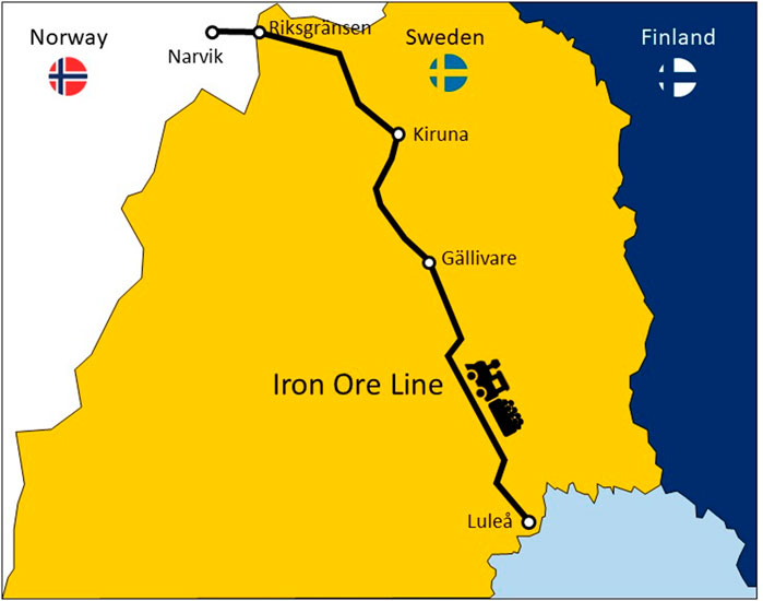
FIGURE 1. Illustration of the Iron Ore Line.

FIGURE 2

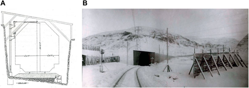
FIGURE 2. Drawing of an early snow gallery from 1913 (A), and picture of a snow gallery from 1913 (B) (Viklund, 2012).

Through this part of the railway, iron ore is transported from LKAB’s mines to the coast of Norway, therefore, it is one of Sweden’s most important transport routes for exporting goods. Delays on this route can be particularly costly, so the snow galleries should be fully functional - neither reparation work nor snow should affect train traffic. This study focuses on two of the sixteen snow galleries between Riksgränsen and Kiruna, built in the 1950s, namely: 9 and 13A.

When these galleries were built, the design snow load was lower than what is required by today’s standards (Swedish Standards Institute (SIS), 2009). Snow loads in Sweden are calculated based on snow depth and density; with time and technology, measuring these parameters became more frequent and accurate, which justifies the changes in calculation. Besides, snow loads are predicted to increase further in the future due to climate change, as higher temperatures will lead to more frequent precipitation in winter, which increases the snow density, and higher probability of extreme snowfalls.

Several snow galleries have been damaged over the years due to excessive snow loads; Sas et al. (2021) reported that the steel sheet and the secondary beams in all sixteen galleries have been damaged, while some of the main frames presented buckling or highly deformed beams (Figure 3). The investigation presented in this paper was then carried out by Luleå University of Technology (LTU) and Swedish Transport Administration (TRV), to prevent similar occurrences in the future.

FIGURE 3

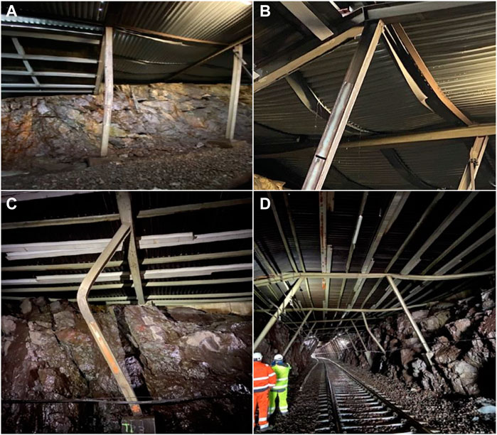
FIGURE 3. Failure of snow gallery 13A (A,B) and failure of snow gallery 9 (C,D) (Sas et al., 2021).

In the context of physical avalanche protection in Switzerland, defensive structures play the most significant role (SLF, 2023). In the Swiss Alps, the earliest evidence of these structures dates back to the 17th century, significantly expanding in the 19th century. A series of major disasters in the winter of 1950/51 prompted a readjustment of avalanche protections, and walls and terraces were replaced by lean and more effective structures made of steel, aluminum, wood, wire rope or concrete (SLF, 2023). Furthermore, the avalanche period of 1968 resulted in massive damage and loss of life, particularly in the region of Davos, to which authorities responded by issuing guidelines for improved hazard maps (SLF, 2023).

In this study, an investigation of snow loads was initially performed, from the history and evolution of snow load calculation in Sweden and other countries, until the prediction of a future overshadowed by climate change. Then, the two snow galleries that were evaluated are presented, as well as the instrumentation of the monitoring system and Finite Element (FE) models. The study proposes an analytical and numerical assessment of the maximum load, displacement and stress supported by galleries 9 and 13A before collapse, with the objective of evaluating how the critical snow load affects the galleries today and may affect them in the future. Analytical calculations were performed according to the Eurocodes and national annexes, and based on documents obtained from TRV’s database, i.e., Sweden’s Bridge and Tunnel Management System (BaTMan). Numerical analysis of the same parameters was performed with both 2D and 3D Finite Element (FE) models, created using AxisVM. The results were compared against live data obtained from the monitoring system installed on both galleries to measure stresses and displacements, as well as temperatures obtained from TRV’s measuring stations. The values obtained from the monitoring system were then correlated with the maximum loads obtained from calculations, and an initial snow load management system was activated. The system includes a warning load and a maximum load and an alert email that was automatically sent when the warning load was triggered.

This study presents originality in the realm of structural engineering and climate science as it delves into the historical evolution of snow load calculations in Sweden and other countries, offering a unique perspective on how these standards have changed over time. This is particularly relevant given the study’s focus on the future implications of climate change on snow loads, an emerging and critical area of research. The multi-disciplinary nature of the research, which integrates structural engineering, climatology, and data science, adds another layer of innovation.

2 Literature review: snow loads

Snow loads are mostly influenced by snow depth and density, which makes it challenging to accurately calculate them, since these parameters depend on factors like location, topography, and weather conditions. Calculation of snow loads in the codes has changed through the years to comply with the evolution of measurement methods of snow parameters, as well as to include other relevant aspects, such roof shape, thermal flow on roofs, and terrain exposure. This means that structures built according to outdated codes might now have lower capacities than what is required by current standards. Besides, actual snow loads are predicted to increase further in the future due to climate change. To better understand and analyze this load, the literature review presented in this section focuses on how snow load has been calculated historically, how it is calculated today, and how the codes may develop to calculate them in the future.

2.1 History of snow load measurements

Snow load in Sweden is calculated from snow depth and density. Snow depth has been systematically measured in Sweden since the beginning of the 19th century (Wern, 2015). The methods have evolved from hand to digital notes, and new measurement technologies have emerged, such as laser and ultrasound. However, none of the automatic stations currently uses them, so all measurements are made by hand in Sweden today. The manual way to measure snow depth consists of vertically inserting a ruler or snow stick into the snow, in a flat surface of about 10 × 10 m where no significant drift has occurred. The number of stations where snow depth is measured in Sweden has grown from about 100 in the 1950s to about 500–700 today. Since 1969, all observations have been registered digitally, and nowadays it is easy to access online the daily snow depth maps provided by the Swedish Meteorological and Hydrological Institute (Swedish Meteorological and Hydrological Institute, 2023).

2.2 Snow density

Snow density is not as widely measured as snow depth, so the local variations are adapted with snow depth measurements. Sweden is divided into three snow density zones, 230, 240 or 280 kg/m³; in northern Sweden, where the snow galleries are placed, the density is 230 kg/m³. Based on a report written by Taesler and Nord (1973) concerning the relation between snow density and depth, a nationwide equation for snow density was compiled (Eq. (1)). Equation (1) describes the mean value of the density of a snow cover ($d\left(t\right)$ in kg/m³), which occurs t days after a common reference date, November 11th.

$\mathit{d}\left(\mathit{t}\right)=\mathbf{0,7}\mathit{t}+\mathbf{155}(1)$

In a report published by Meløysund et al. (2007), six different variables and their influence on snow density were analyzed, namely: snow depth, atmospheric pressure, precipitation, air humidity, solar radiation, and high wind speed. The study found that the greatest effect on snow density was the relative air humidity while it is snowing. Furthermore, snow depth, atmospheric pressure, and precipitation were identified as factors that decrease snow density, while air humidity, solar radiation, and high wind speed increase the density. Still according to Meløysund et al. (2007), the mean bulk weight density of snow values given by SIS (2009) are overestimated, and the density formulas from International Organization for Standardization, 1998 are not applicable unless extremely rough estimates are to be made.

The current snow load map was calculated from a series of measurements of snow depth from measuring stations across the country (Boverket, 2020). A Gumbel distribution was used with assumptions of snow density at maximum snow depth, and an average return period of the loads of 50 years within the 98-percentile. The snow depth is measured at 148 stations and the map is adjusted with isolines between these stations, the snow load in a specific point is then taken as the mean value of two isolines. Johansson and Ericsson (2019) evaluated the accuracy of this method and the Gumbel distribution was deemed sufficient; however, if the proportion of variable load exceeds 60% of the total load, the probability of structural failure is higher than allowed by the regulations.

2.3 Snow cover

Snow cover refers to the area of the land covered by snow. Taesler and Nord, (1973) and Sturm (2020) discuss snow depth and density, which are the most fundamental characteristics of the seasonal snow cover. During a season, research shows that snow density increases linearly, except for the start and end of the season, where the density has slightly higher values. The product of the snow depth and density is the areal density, which is often referred to as the snow water equivalent (SWE) in kg/m². Historical information about snow depth is common, while measurement data on density and SWE is rare, which makes it difficult to perform statistical calculations today.

Taesler and Nord, (1973) also investigated how the maximum values for snow density and depth coincide during a season. In northern Sweden, both values increase during the winter and reach their maximum in the end of the season. On the other hand, maximum snow depth occurs before maximum density in reached in southern Sweden. This difference is due to precipitation: in the north, when snow depth is at its maximum, precipitation is low; however, in the south precipitation can occur when snow cover is at its maximum and increase its density over time.

Based on the findings reported by Taesler and Nord, (1973) and Sturm (2020), Table 1 summarizes the main processes that influence the properties of the snow cover.

TABLE 1

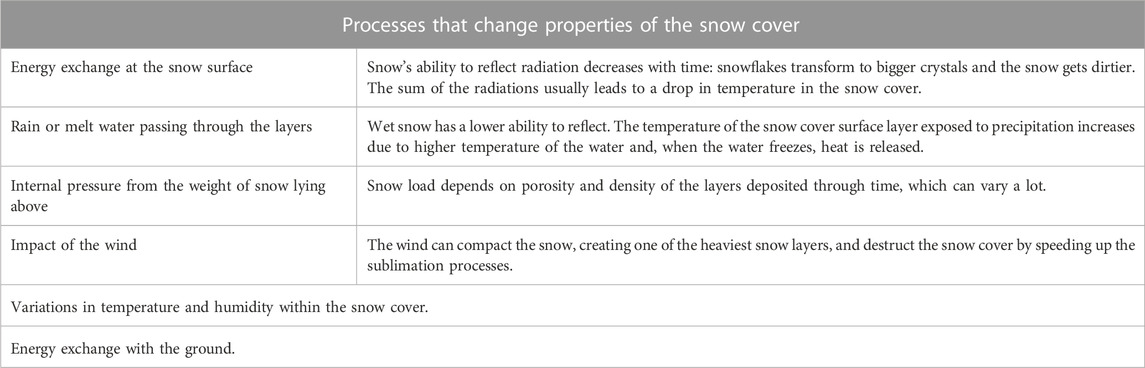
TABLE 1. Processes that change properties of the snow cover.

2.4 Evolution of snow loads in Swedish standards

The first national snow load code was established in Sweden in 1946 with the first BABS standard, BABS46 (Boverkets, 1946). In 1968, the BABS standards were replaced by the SBN standards (Boverket, 2023a) until 1989, when the NR standards (Boverket, 2023b) replaced those. In 1994, NR is then replaced with BBR and BKR (Boverket, 2023c), until 2007, when Eurocode regulations were introduced in Sweden. Exceptional snow loads were mentioned for the first time in national regulations when Sweden introduced the Eurocodes. When the national annexes were created, it was decided that exceptional snow loads would not be considered, since that weather phenomenon was not relevant to the Swedish climate. However, a note was included in the Swedish annex that if higher reliability is desired for a building in open terrain, where high wind strengths can arise, snow drift can be considered as an accidental load.

Figure 4 presents the evolution of the snow load codes in Sweden, accounting for the main changes from one code to the follower. Figure 4 references the snow load maps in Table 2, which presents the evolution of snow load maps in Sweden, numbered as I, II, III, IV and V. From the snow load maps, Table 3 presents the changes in the snow load calculated for a single pitch roof in Luleå, the starting point of the Iron Ore Line (Figure 1). When designing structures today, it is possible to access the SMHI’s (Swedish Meteorological and Hydrological Institute) real time snow load map online, under the website: https://vattenwebb.smhi.se/modelsnowload/client/.

FIGURE 4

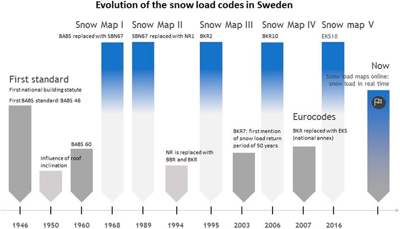
FIGURE 4. Evolution of snow load codes in Sweden.

TABLE 2

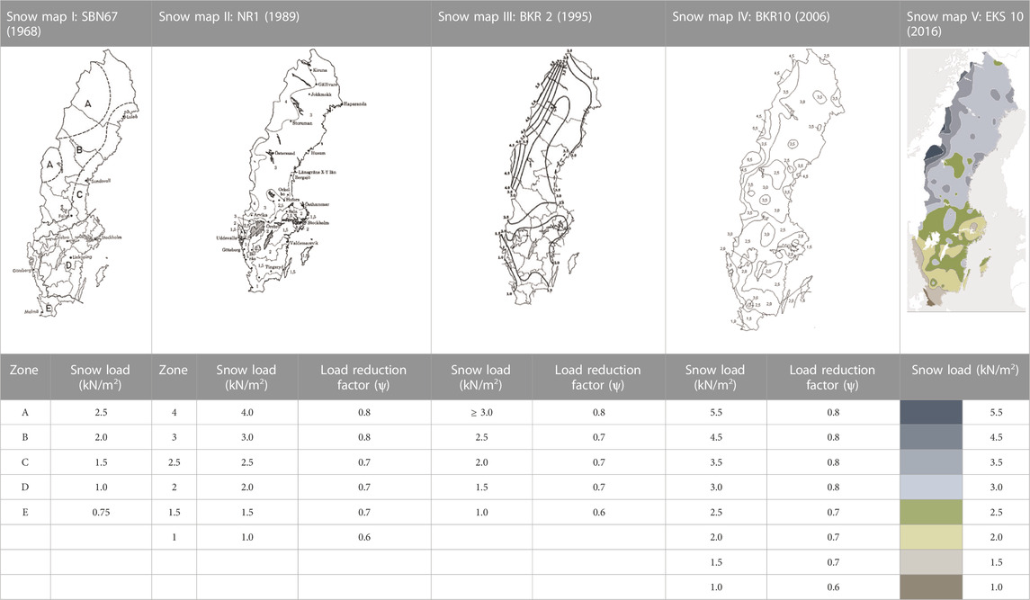
TABLE 2. Evolution of snow load maps in Sweden (Boverket, 1968; Boverket, 1988; Boverket, 1995; Boverket, 2006; Boverket, 2023d).

TABLE 3

TABLE 3. Changes in the snow load on a single pitch roof calculated according to the evolution of snow load maps.

2.5 Snow load calculation: Eurocode and the Swedish standard

Design snow loads on roofs and on the ground are currently calculated in Sweden from Eurocode 1–Actions on structures–Part 1–3: General actions–Snow loads and the National Standard SS-EN 1991-1-3/A1:2015 (Swedish Standards Institute, 2009a). Snow load is considered as a variable load, classified as a static action. For snow load on roofs, the design load is calculated according to Eq. 2.

${\mathit{s}}_{\mathit{d}}={\mathit{\mu }}_{\mathit{i}}\bullet {\mathit{C}}_{\mathit{e}}\bullet {\mathit{C}}_{\mathit{t}}\bullet {\mathit{s}}_{\mathit{k}}(2)$

Where $s_d$ is the design snow load on the roof; ${\mu }_i$ is the snow load shape coefficient; $C_e$ is the exposure coefficient; $C_t$ is the thermal coefficient; and $s_k$ is the characteristic value of snow load on the ground.

The exposure coefficient ($C_e$) depends on the topography of construction site: windswept ($C_e=\mathrm{0,8}$), normal ($C_e=\mathrm{1,0}$) or sheltered ($C_e=\mathrm{1,2}$). In windswept areas, nothing prevents the wind from affecting the building, while sheltered areas are surrounded by higher buildings or terrain that protect the building from the wind. The shape coefficient (${\mu }_i$) depends on whether the roof is monopitch or pitched, the inclination of the roof and the number of spans. Graphs and tables for different conditions are presented on both the Eurocode (European Committee for Standardization, 2003) and the National Annex (Swedish Standards Institute, 2009b). The thermal coefficient accounts for the reduction of snow loads due to melting on roofs with high thermal transmittance, in particular some glass covered roofs, but in all other cases: $C_t=\mathrm{1,0}$.

Regular characteristic ground snow load ($s_k$) is obtained from snow load maps, and, for special cases, Eurocode 1 recommends that the value is determined from statistical analysis of long records taken in an area near the site. The European Commission has divided Europe into different climate regions–the region corresponding to Sweden and Finland is presented in Table 4. For each region, the load is then calculated using Eq. 3, which considers the altitude (A) and the location represented by the zone number (Z).

${\mathit{s}}_{\mathit{k}}=\mathbf{0.790}\mathit{Z}+\mathbf{0.375}+\frac{\mathit{A}}{\mathbf{336}}(3)$

TABLE 4

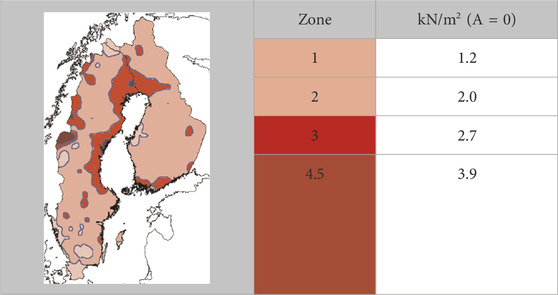
TABLE 4. Snow load at sea level: Sweden, Finland region. Adapted from SIS (2009).

Finally, the design loads are calculated from the Ultimate Limit State (ULS) combinations in SS-EN 1990 (Swedish Standards Institute, 2009c) presented in Table 5. In the equations, the number multiplied by load accounts for the possibility of unfavorable deviations of the load, and the γ_d coefficient accounts for the uncertainty of the load effect model. The design load is calculated from whichever combination generates the highest load.

TABLE 5

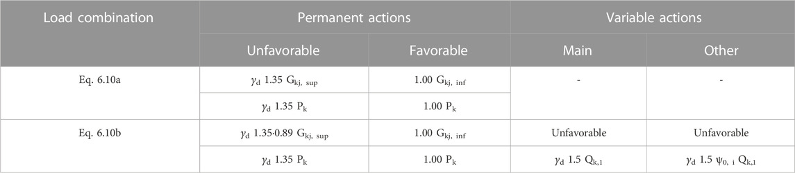
TABLE 5. Load combinations according to EKS 11 (2019).

2.6 Snow load calculation: other countries

In other regions of Europe covered by the Eurocodes, the snow load is calculated from snow maps similarly to Eq. 3. In the United States, the relationship between snow depth and snow load has been established through Eq. 4, which also considers that the maximum snow load and maximum snow depth do not occur on the same day.

${\mathit{s}}_{\mathbf{50}}=\mathbf{1,91}{\left({\mathit{d}}_{\mathbf{50}}\right)}^{\mathbf{1,33}}(4)$

Where $s_{50}$ is the ground snow load (in kPa) with a return period of 50 years; and $d_{50}$ is the snow depth (m) on the ground with a return period of 50 years.

Measurements of the water content in the snow should be used when determining the snow load. However, since this data is uncommon to measure, snow depth measurements can be used if the data is not sufficient. Therefore, methods to calculate snow density from snow depth have been developed, such as Eq. 5 (United States), Eq. 6 (Russia), Eq. 7 (Japan), and Eq. 8 (Germany).

$\mathit{\rho }=\left\{\begin{array}{c}\frac{\mathbf{270}}{\mathbf{1,2}-\mathbf{0,51}\mathit{d}};\mathit{d}<\mathbf{1,25}\mathit{m}\\ \mathbf{480};\mathit{d}\ge \mathbf{1,25}\mathit{m}\end{array}\right.(5)$

Where $\rho$ is the snow density (kg/m³); and $d$ is the snow depth (m).

$\mathit{\rho }=\left(\mathbf{90}+\mathbf{130}\sqrt{\mathit{d}}\right)\left(\mathbf{1,5}+\mathbf{0,17}{}^{\mathbf{3}}\sqrt{\mathit{T}}\right)\left(\mathbf{1}+\mathbf{0,1}\sqrt{\mathit{v}}\right)(6)$

Where $\rho$ is the snow density (kg/m³); $d$ is the snow depth (m); $T$ is the average temperature (°C) over the period of snow accumulation (not lower than −25°C); and $v$ is the average wind velocity (m/s) in the same period.

${\mathit{\rho }}_{\mathit{e}}=\mathbf{73}\sqrt{\raisebox{1ex}{$\mathit{d}$}\!\left/ \!\raisebox{-1ex}{${\mathit{d}}_{\mathit{r}\mathit{e}\mathit{f}}$}\right.}+\mathbf{240}(7)$

Where ${\rho }_e$ is the equivalent snow density (kg/m³); $d$ is the snow depth (m); and $d_{ref}$ is the reference snow depth of 1 m.

$\mathit{\rho }=\frac{{\mathit{\rho }}_{\mathit{\infty }}{\mathit{d}}_{\mathit{r}\mathit{e}\mathit{f}}}{\mathit{d}}\mathit{ln}\lceil \mathbf{1}+\frac{{\mathit{\rho }}_{\mathbf{0}}}{{\mathit{\rho }}_{\mathit{\infty }}}\left(\mathit{exp}\left(\frac{\mathit{d}}{{\mathit{d}}_{\mathit{r}\mathit{e}\mathit{f}}}\right)-\mathbf{1}\right)\rceil (8)$

Where ${\rho }_0$ is the density of snow at the surface (kg/m³); ${\rho }_{\infty }$ is the upper limiting value of the snow density; $d$ is the snow depth (m); and $d_{ref}$ is the reference snow depth of 1 m. For Germany, the snow density at the surface (${\rho }_0$) usually is in the range from 170 kg/m³ (dry climates) to 190 kg/m³ (wet climates), and the upper limiting value (${\rho }_{\infty }$) ranges from 400 kg/m³ (dry climates) to 600 kg/m³ (wet climates).

The International Organization for Standardization (ISO) (2013) states that a table, formula, or map based on statistical measurement results for the ground snow load should be available for each country in their national standards. They recommend against the use of isolines; instead, they recommend dividing the country into zones according to the height above sea level and to the distance to the coast, as these are factors of great influence to the snow load. In the newer standard, the updated equation for calculating snow load with a return period of 50 years is presented in Eq. 9, which represents an increase from the previous equation (Eq. 4).

${\mathit{s}}_{\mathbf{50}}=\mathbf{1,97}{\left({\mathit{d}}_{\mathbf{50}}\right)}^{\mathbf{1,36}}(9)$

Figure 5 presents a graph compiling snow density calculations using Eqs 5–8 from different countries. Two alternatives are shown for Eq. 6, from Russia: average temperature of −10°C and −20°C for a constant wind speed of 4 m/s. For Eq. 8, from Germany, two alternatives are also presented: dry climates (${\rho }_0$ = 170 kg/m³ and ${\rho }_{\infty }$ = 400 kg/m³) and wet climates (${\rho }_0$ = 190 kg/m³ and ${\rho }_{\infty }$ = 600 kg/m³).

FIGURE 5

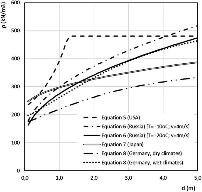
FIGURE 5. Snow density calculations from different countries. Adapted from International Organization for Standardization, 2013.

2.7 Impact of climate change

When calculating snow load zones, International Organization for Standardization, (2013) recommends considering the risk of the impact of climate change. Extreme values can be expected in both directions and adjustments should be made according to the trend in different scenarios. The Swedish Meteorological and Hydrological Institute has reported on the impact of climate change in Norrbotten, in northern Sweden (Swedish Metereological and Hydrological Institute, 2015). The reported scenarios are based on the greenhouse gas concentration trajectories, called Representative Concentration Pathways (RCP), adopted by the Intergovernmental Panel on Climate Change (IPCC). The RCP are four different pathways used for climate modeling and describing possible climate futures, varying with the volume of greenhouse gases emitted in the period considered in the analysis. The calculations in the report consider RCP4.5 and RCP8.5, which represent a possible range of radiative forcing values of 4.5 and 8.5 W/m², respectively.

Climate change effects and temperature rise are more frequent than before and might impact the future. Higher temperatures lead to an increase in water evaporation, which leads to more precipitation. The annual average precipitation is assumed to increase by 20% for RCP4.5, and by 40% for RCP8.5, with the largest increase occurring in the mountain areas. The maximum daily precipitation is also predicted to increase by 15%–25%, depending on the RCP scenario. Higher temperatures and more frequent precipitation can decrease the snow cover but elevate its weight. Besides, the extreme meteorological phenomena are also believed to increase in probability, which can imply more often extreme snowfalls, despite a decreased amount of snow in general (Strasser, 2008; Swedish Metereological and Hydrological Institute, 2015).

Croce et al. (2021) also performed similar simulations for Europe, considering scenarios RCP4.5 and RCP8.5, and their results indicated a reduction of the annual maxima and an increase on the standard deviation of snow loads. Locally, the results pointed to higher extreme values and showed that the snow load in the mountain ranges in Scandinavia will exceed current loads (Croce et al., 2021).

3 Case study and methodology

The snow that falls and builds on the cover of the snow galleries generates stress, strain, and deformation on the structural system. A monitoring system was installed on galleries 9 and 13A to measure loads and deformations, while temperatures were simultaneously obtained from nearby measuring stations. To determine the critical loads on the steel frames, calculations and numerical FE models were developed. A site visit was also conducted in March 2022, when the snow galleries were loaded with snow, to observe how the snow accumulates around the walls and on the roof of the galleries, due to local geometry and landscape layout. Figure 6 presents the methodology flowchart for the study, and this section presents the galleries, the monitoring system, the calculations, and models created to support the analysis in this study.

FIGURE 6

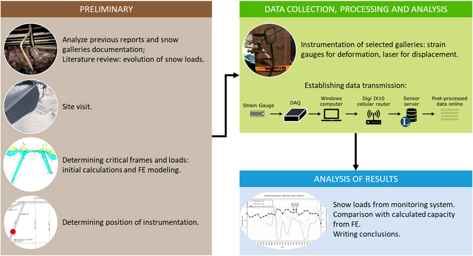
FIGURE 6. Methodology flowchart.

The limitations of this study are:

• Snow loads and snow density were calculated based only on theory and regulations.

• Imperfections of the frames were not considered.

• The models were based on the original drawings from The Swedish Transport Administration, structural changes and repairs performed throughout the years were not considered.

• Avalanche loads were neglected.

• The stabilizing effect of the steel sheet on the secondary beams was neglected.

3.1 The galleries

Two of the sixteen snow galleries between Riksgränsen and Kiruna were analyzed in this study, namely: SG9 and SG13A. The length of each gallery varies between 118 and 642m, and in total there are 3.9 km of snow galleries. From the original drawings, the galleries have two structural parts: a main frame composed of laminated steel profiles (types I, H, Z), and secondary elements, i.e., prefabricated concrete slabs or secondary beams covered by steel sheets. The bay spacing for the main frames is 5–6 m (SG13A) or 7.5 m (SG9), and their geometry mostly depends on the local landscape conditions. Throughout the years, the galleries have been strengthened or replaced without respective updates to the original drawings, so today there is no complete documentation of all the modifications performed in time.

SG13A is 225 m long, it is constructed with 54 frames, and it is located at the station in Vassijaure. The first part SG13A was built in 1952, and it has been extended in two directions on two different occasions. In 1955, SG13A was extended towards Riksgränsen, and in 2003 came a new extension towards Vassijaure. In 1979, covering was replaced with steel sheeting, placed on secondary beams (Z-beams, height: 200 mm) between the frames (concrete retained on the walls). Figure 7 presents the evolution of the extensions added to SG13A, including drawings of the main frame in the early structure and in the newest extension. The monitoring system was installed on frame +420, illustrated in Figure 7.

FIGURE 7

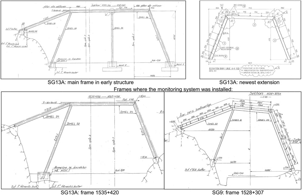
FIGURE 7. Original drawings from the snow galleries and frames on which the monitoring system was installed.

SG9 is 217 m long, it was constructed in 1954 with 29 frames every 7.5 m. At first, the frames were covered with Eternit plates, but after renovations the gallery is now covered with steel sheets and some secondary beams have been replaced. The monitoring system in SG9 is placed on frame +307 (Figure 7).

3.2 Finite Element modelling

A linear FE analysis was conducted using AxisVM, with both 2D and 3D finite element models. The 3D analysis was included with the main goal of evaluating the influence of the frames over each other because of the cobweb effect, which consists of the re-distribution of the stresses between the structural elements due to the tri-dimensional interaction. The FE models were created based on the original drawings and on direct observations. However, due to lack of information, some assumptions had to be made based on notes from the original drawings and on the report by Sas et al. (2021). All assumptions are presented in the following section, as well as the method and considerations applied to develop the FE models used in the analysis.

3.2.1 Materials, geometry, and boundary conditions

For the materials, structural steel S275 ($f_y$ = 275 MPa) was chosen for the main structural system and S235 ($f_y$ = 235 MPa) was assumed for the secondary structural system, based on the notes in the original plans. To create the models for the numerical analysis, the geometry of the frames was extracted from the original drawings from the 1950s.

For the boundary conditions, the nodal degree of freedom was set to a free node. For the 2D analysis, the program required some adjustments to run the model and extra nodal degrees of freedom had to be included to stabilize some of the frames, since the stabilizing effect of the secondary beams was neglected in the 2D analysis.

Two types of supports were established for the columns: a rigid support, in which the pillar is attached to the rock or plinth and cast in, and a hinge support, in which the pillar is only fastened with two bolts. The original drawings of the supports, a picture of each type on site, and the schematic representation are shown in Figure 8.

FIGURE 8

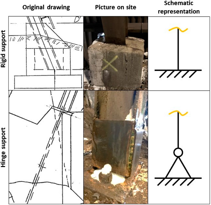
FIGURE 8. Supports: in the original drawings, on site and schematic representation.

For the primary beams, all the connections are welded and were therefore assumed to act like moment connections, which allow the transfer of bending moments between elements. The secondary beams are also welded on top of the main frames and were analyzed as simply supported beams, since the connections were deemed insufficient to handle bending moment. However, in SG13A there are indications that the cold formed secondary Z-beams overlap each other and are bolted together, and this connection to the main frames can be assumed as a moment connection, so calculations were performed for both scenarios.

The permanent loads considered were the self-weight from the main frame and the roof coverings. The self-weight of the main frame was automatically calculated in the program. There are two types of roof covering: for the steel sheet, the load was calculated according to Equation 10, and for the concrete slab, the load was calculated according to Equation 11. The distances used for the load calculations are illustrated in the example frame shown in Figure 9. The permanent loads were included in the program with the following parameters: ${\gamma }_{G,\mathit{sup}}$ = 1.35; ${\gamma }_{G,\mathit{inf}}$ = 1.00; and $\xi$ = 1.00.

${\mathit{g}}_{\mathit{k},\mathit{s}\mathit{t}\mathit{e}\mathit{e}\mathit{l}}=\mathit{a}*\mathit{w}\left({\mathit{g}}_{\mathit{b}\mathit{e}\mathit{a}\mathit{m}}+{\mathit{g}}_{\mathit{s}\mathit{h}\mathit{e}\mathit{e}\mathit{t}}*{\mathit{w}}_{\mathit{m}\mathit{e}\mathit{a}\mathit{n}}\right)(10)$

Where: $g_{k,steel}$ is the load from the steel sheet roof covering [kN]; $a$ is the gravitational acceleration [m/s²]; $w$ is the distance between the main frames [m]; $g_{beam}$ is the self-weight of the secondary beam [kg/m]; $g_{sheet}$ is the self-weight of the steel sheet, assumed as 20 kg/m²; $w_{mean}$ is the mean distance between the secondary beams [m].

${\mathit{g}}_{\mathit{k},\mathit{c}\mathit{o}\mathit{n}\mathit{c}}=\mathit{\rho }*\mathit{t}*\mathit{w}(11)$

Where $g_{k,conc}$ is load from the concrete slabs [kN/m]; $\rho$ is the density of reinforced concrete [kN/m³]; $t$ is the thickness of the concrete slab, given in the original drawings as 0.065 m; and $w$ is the distance between the main frames [m].

FIGURE 9

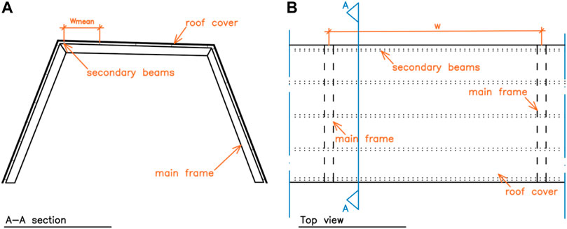
FIGURE 9. Example frame with distances for load calculations, section view (A) and top view (B).

The variable loads considered were wind and snow loads. Upon analysis, the wind load contributed mostly as suction force, which acted as a favorable load in combination with the snow load, so it was neglected in the evaluation. The snow loads were calculated according to Eq. 2, from Eurocode, considering the inclination of the beams. The following variable load parameters from Eurocode for the regions of Sweden, Finland, Norway, and Iceland were used: ${\gamma }_Q$ = 1.5 (EN 1990 Annex A.1, Table A1.2); ${\psi }_0$ = 0.7, ${\psi }_1$ = 0.5, ${\psi }_2$ = 0.2 (EN 1990 Annex A.1, Table A1.1). The safety coefficient (${\gamma }_Q$ = 1.5) was adjusted to 1,0 to compare the snow loads with the characteristic values obtained from the monitoring system. Table 6 presents a summary of the considered parameters.

TABLE 6

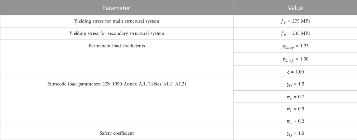
TABLE 6. Summary of considered parameters.

Table 7 presents the load combinations put together by AxisVM, used for the load calculations. The most critical combination was selected to analyze all the frames. Then, for each snow gallery, analyses were performed for the most critical frame, selected based on the degree of utilization, as well as the frame in which the monitoring system was installed. For these two frames, further analyses were conducted to draw conclusions on the maximum capacity and establish the critical snow loads. The normal force on the columns was calculated only for the snow load to enable the comparison with the values obtained from the monitoring system, since the system was calibrated when the column was loaded with self-weight.

TABLE 7

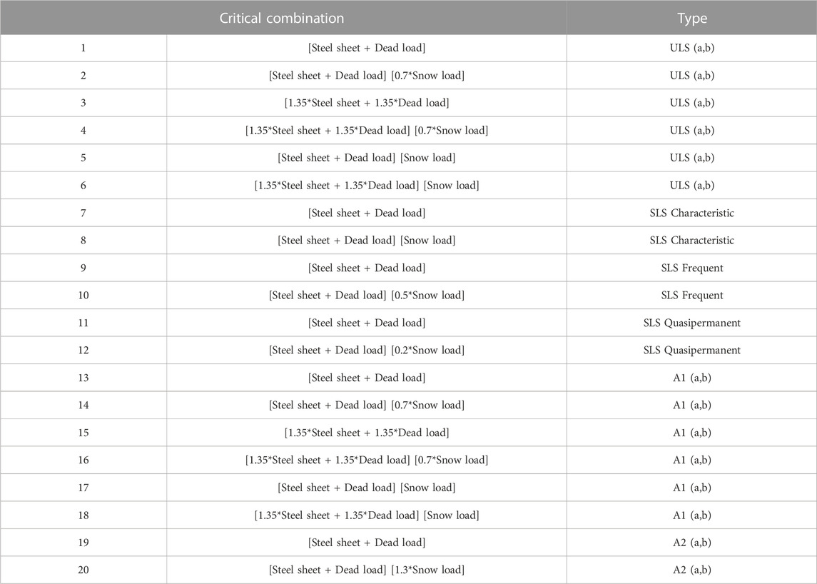
TABLE 7. Load combinations with safety factor of 1,0 for snow load.

3.3 Monitoring system

The monitoring equipment for each gallery consisted of strain gauges, a laser beam to measure deflection, and temperature information was also obtained from nearby measuring stations. Permanent electrical connection was provided on site to enable continuous measurements–in case of power fail, a backup battery can sustain for a short period. Frame +420 was instrumented in SG13A, and frame +307 was instrumented in SG9.

The laser beam was installed directed towards the roof beam on both galleries to measure deflection. Two strain gauges were attached with resistance spot welding to the monitored column on each gallery, one in the x direction and one in the y direction. Before installing the strain gauges, the surface was polished with an angle grinder, a belt sander and polishing paper. To calibrate the strain gauges, two load cells and two hydraulic jacks were used on each side of the DIMEL-column, equally loaded on both sides. The beam was first loaded with up to 5,000 kg, when the load was measured, then it was increased to 10,000 kg, when the load was measured again. After that, the load and the loading equipment were removed. For accurate interpretation of load measurements by the system, the calibration loads must exceed the anticipated snow loads the system will measure.

To determine the maximum stress sections for the optimal position for the laser beam and strain gauges, FE analyses were performed using AxisVM for both galleries. On both frames, strain is measured on the center column and deflection is measured on the left column. Figure 10 presents the displacement and stress FE analysis as well as the position of the laser beam and strain gauges for both galleries. Figure 11 presents a picture of the placement of the strain gauges, the putty protection cover, and the laser beam directed to the roof beam.

FIGURE 10

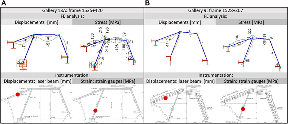
FIGURE 10. Instrumentation on SG13A (A) and 9 (B): FE analysis, position of laser beam and strain gauges (red dot).

FIGURE 11

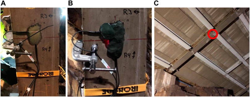
FIGURE 11. Placement of strain gauges (A), covered with putty (B), and laser to measure deflection (C).

The output from the system consists in absolute values for deflection, column stress and ambient temperature, all available through an online permanent access link. The column load is calculated from the strain measured by the strain gauges, and if its value reaches a limit value of 80kN, a warning message was triggered, and an email was sent to an assigned maintenance team.

The setup for the system comprises a Windows-based computer linked to the HBM Spider8 data acquisition (DAQ) unit. The HBM Spider8 is a real-time data acquisition solution with analog and digital input channels, facilitating connections to various sensors. A Digi IX10 cellular router establishes the mobile network connection for data transfer. One hundred samples are collected every 10 min and exported to an ASCII file. This file is then transmitted to LTU’s MCE-LAB server (Linux CentOS). Next, snow load data is post-processed by extracting median, minimum, and maximum values. These processed values, along with temperature data constantly sourced from temperatur.nu (2023) via the Swedish Road Administration’s weather service, are exported to a website, ensuring online accessibility.

4 Results

This section presents the results obtained from the finite element 2D and 3D calculations, the monitoring system installed in galleries 9 and 13A, as well as a site visit from March 2022.

4.1 FE analysis

4.1.1 2D analysis

The 2D analysis was performed for all the frames in both snow galleries, but here will be presented only the most critical frame and the frame in which the monitoring system was installed in galleries 13A and 9. From the 2D analysis, stresses, axial loads, and utilization ratios were obtained for the frames.

In SG13A, the most critical section was frame +460, and in SG9, it was frame +292. The frames were initially loaded with the characteristic snow load of $s_k$ = 4.5 kN/m², as recommended by Boverket (2022) for the corresponding area. The load was later reduced to 3.1 kN/m² in SG13A and to 1.65 kN/m² in SG9 to achieve a utilization ratio of less than 1.0. Figure 12 presents the snow loads, stresses, and utilization ratios (numbers inside colored squares) for critical frames +460 and +292.

FIGURE 12

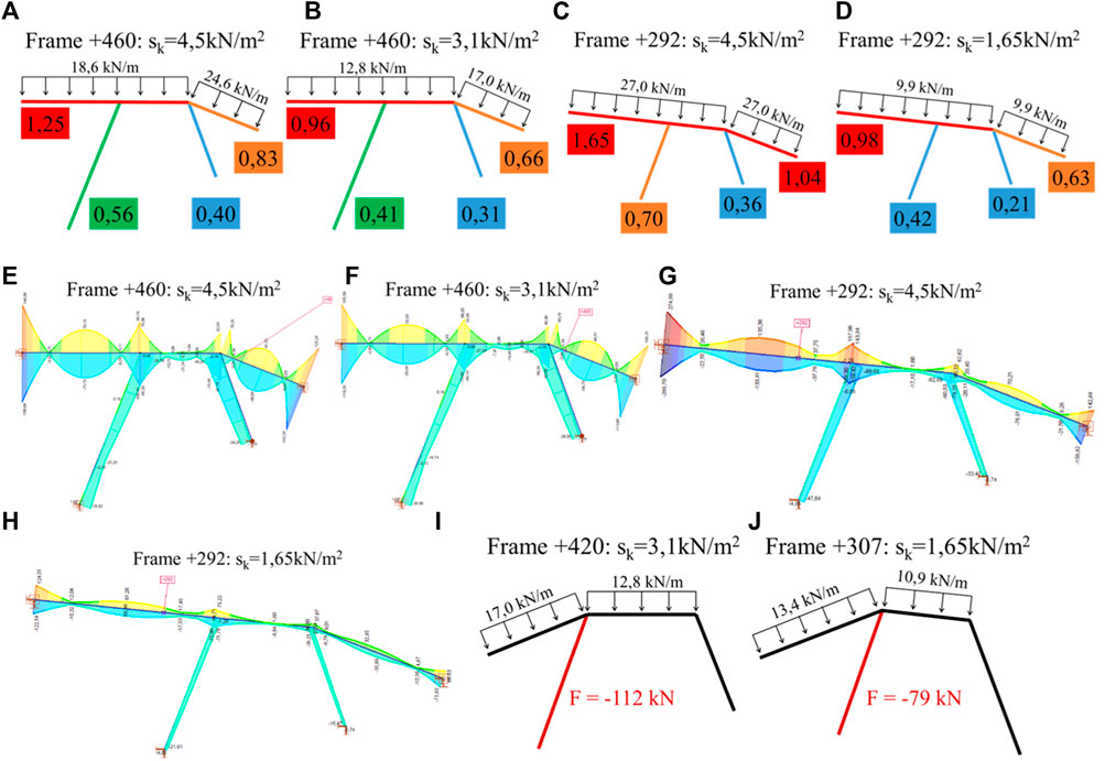
FIGURE 12. Utilization ratio (numbers in colored rectangles) in most critical frames: frame +460 (A) s_k = 4.5 kN/m² and (B) s_k = 3.1 kN/m²; frame +292 (C) s_k = 4.5 kN/m² and (D) s_k = 1.65 kN/m². Stresses in most critical frames: frame +460 (E) s_k = 4.5 kN/m² and (F) s_k = 3.1 kN/m²; frame +292 (G) s_k = 4.5 kN/m² and (H) s_k = 1.65 kN/m². Axial force in monitored column in the frames with the monitoring system: (I) Frame +420 (SG13A) and (J) Frame + 307 (SG9).

The monitoring system was installed on frame +420 in SG13A and on frame +307 in SG9. In frame +420, the axial force in the monitored column was 112 kN, and in frame +307, 79 kN. Figure 12 also presents the snow loads and axial force in the monitored column for frames +420 and +307. In the figures, the sign (-) is used to represent compression forces.

4.1.2 3D analysis

Similarly to the 2D analysis, the outcome of the 3D FE analysis were the stresses, axial load, and utilization ratio. The 3D analysis identified frame +390 as the most critical in SG13A, sustaining a snow load of 7.1 kN/m² before failure. This load yielded a normal force in the monitored column (frame +420) of 232 kN. For SG9, the 3D analysis identified frame +247 as the most critical, sustaining a snow load of 2.3 kN/m² before failure. In the frame with the monitoring system (+307), this load yielded a normal force in the monitored column of 164 kN.

Figure 13 presents the 3D model of galleries 9 and 13A, in which the green squares represent the concrete slabs, and the blue ones represent the steel sheets. The monitored frames +420 and +307, respectively for SG13A and SG9, are also highlighted in Figure 13. Figure 14 presents the utilization ratio in the critical frames under the critical loads identified by the 3D analysis in galleries 13A and 9. Figure 14 also presents the axial force in the monitored column for frames +420 and +307.

FIGURE 13

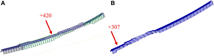
FIGURE 13. 3D model of SG13A (A) and 9 (B)–full model that included all the steel frames.

FIGURE 14

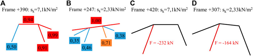
FIGURE 14. Utilization ratio: frame +390, s_k = 7.1 kN/m² (A); frame +247, s_k = 2.33 kN/m² (B). Axial force in monitored column in the frames with the monitoring system: (C) Frame +420 (SG13A) and (D) Frame +307 (SG9).

In the 3D analysis, the secondary beams were also evaluated in both galleries. In SG13A, two scenarios were considered for the end supports of the secondary beams: both fixed and both hinged. With fixed supports, the most critical stress distribution occurred on frame +390. The secondary beams in that frame were able to sustain a maximum snow load of 0.85 kN/m². Applying this load to the frame in which the monitoring system was installed (+420), the load in the monitored column was 27.3 kN. With hinge supports, the most critical stress distribution occurred on frame +380. The secondary beams in that frame were able to sustain a maximum snow load of 0.50 kN/m². Applying this load to frame +420, the load in the monitored column was 15.8 kN.

In SG9, the secondary beams were assumed to have hinged supports. It was identified that the capacity of the roof beams had been exceeded for most of secondary beams. It was observed that the side beams were arranged on the sides in a way that the snow loads were applied on the minor inertial axis. When applying a snow load as little as 0.1 kN/m², the utilization ratio was already more than 100% on most of them. The analysis of the stress distribution showed that the stress level had not been exceeded on the roof beams, but on the walls. The stress distribution varied depending on the inclination of the walls where the secondary beams are attached.

4.1.3 3D analysis: summary of critical loads

The 3D analysis was conducted to assist the calculations and to analyze the cobweb effect due to the interaction of the frames. A color code system was created to facilitate interpretation of the results, including three different load zones: green, yellow, and red zones. Loads in the green zone are below the capacity of all main frames and secondary beams. In the yellow zone, the capacity of the main frames is still sufficient, but the secondary beams have reached their load-bearing capacity. In the red zone, the main frames as well as the secondary beams have reached their load-bearing capacity. Table 8 presents the critical load values for each zone in both galleries.

TABLE 8

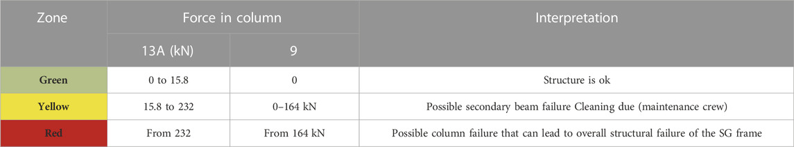
TABLE 8. Critical load zones for galleries 13A and 9: color code system.

4.2 Monitoring system

The outcome of the monitoring system consists of strains measured by the strain gauges, deflections, measured by the laser beam, and temperature, obtained from nearby stations. From the measured strain, the load is calculated and presented as another outcome. Unfortunately, the deflections did not present reliable readings, so this parameter was excluded from further analysis. The results from the monitoring system are presented as graphs containing the minimum and maximum temperatures measured in snow galleries 9 and 13A, as well as the snow load (axial force in the column calculated from the measured strains). The maximum axial force in the columns seen in the graphs corresponds to the red and green zones limit loads seen in Table 8, considering the loss of stability as well as the axial stress. Bending moments are transferred through the moment connections in the frames.

The graphs presented in Figure 15 correspond to the months of February and March 2022. During the winter, however, some faults occurred as the equipment needed to be reprogramed, which lead to missing few data points. The dates in February in which the snow was cleaned from the galleries are marked in the corresponding graphs, although it is possible that other unregistered snow cleaning activities have occurred. In the graphs, it is possible to see that days with lower temperatures lead to increased snow loads.

FIGURE 15

FIGURE 15. Monitoring system results for: (A) SG9 in February, (B) SG9 in March, (C) SG13A in February, (D) SG13A in March.

4.3 Site visit

A site visit was held on March 2022 to complement the analysis with observations from the snow galleries. The main observations are listed as follows and illustrated in Figure 16.

• Snow had accumulated on the lower parts of the gallery walls, mostly due to the wind blowing from the mountain side, and significant variations in snow depth were observed.

• There had been heavy rain prior to the visit, which created a rock-hard layer of ice right below the outer layer of powder snow, so it was not possible to measure snow depth during the visit.

• Snow pockets were formed where roofs were clamped directly into rocks and where the gallery dimensions changed. Snow accumulation increased towards these pockets.

• Snow did not accumulate significantly on narrow roofs, but it did so on wider gallery roofs without distinct walls. Side roofs at an angle of about 20° were fully covered in snow.

• A reparation had been done inside SG13A during previous years, in the roofs of frames +435 to +470. Both secondary beams and concrete slabs were removed and replaced by I-beams and steel sheets.

FIGURE 16

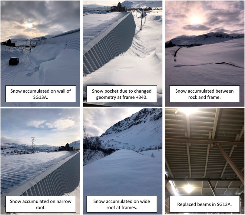
FIGURE 16. Pictures and observations from site visit.

5 Discussion

5.1 Analysis of results

By analyzing the results of the monitoring system, seen in Figure 15, the forces on the columns were far from reaching the red zone loads. Even though the yellow zone has been reached, which means the critical load was exceeded for the secondary beams, no collapse has taken place in the galleries. This can indicate that the secondary structure has been repaired or replaced, and therefore has greater capacity than the model indicated.

The critical load obtained from the 2D FE models for both galleries 9 and 13A was lower than current Swedish regulations, therefore, these galleries cannot handle the applicable standard loads. When they were built, the characteristic snow load should have been set to 2–3 kN/m², which is close to their bearing capacity: 1.65 kN/m² for SG9 and 3.1 kN/m² for 13A. The most common and critical stability problem for the gallery frames is lateral torsional buckling, some of the frames are also unstable due to insufficient support conditions without the secondary beams.

The galleries have not collapsed even though the loads they are subjected to are higher than what the calculations show that they can handle. A possible explanation is that the secondary beams stabilize the frames by creating a cobweb effect for the whole gallery. This hypothesis was tested with the 3D FE model, which showed that the cobweb effect had a great impact on the galleries, resulting in different critical frames and critical loads.

When creating the model, it was assumed that the snow load acting on the steel sheet roof cover is transferred to the secondary beams, and then to the main frames. This assumption corresponds to the in-plan analysis done in the 1950s, when the galleries were designed. It is now known that the steel sheet’s capacity is lower than the secondary beams’ capacity, which is lower than the main frames. The fact that the outer construction elements (secondary beams and steel sheeting) have damaged before the main frames have reached their capacity means that the main frames were prevented from supporting higher loads; the secondary elements acted as a safety fuse for the main frames.

Lastly, the load from snow accumulated around the galleries was analyzed. Snow accumulates at the foot of the gallery walls, snow pockets form where the structure changes geometry, and snow pushed by the wind from the mountain accumulates towards the galleries. However, it was concluded that after the snow has settled, this load does not lead to significant pressure on the construction.

5.2 Snow load evaluation

Upon evaluation of regulations for different countries over time, it became evident that snow loads are scientifically difficult to calculate. They vary between different geographical areas, and they can change depending on climate and location within those areas. Snow thickness can be straightforward to measure and is a main parameter when calculating snow loads. Snow density, however, is of even more importance in calculations and is much more complicated to obtain. No consensus has been reached regarding the parameters that affect snow density, and different standards take different parameters into account. Researchers agree that the density increases with time and the maximum density does not coincide with the maximum snow depth. The density currently used for load calculations in Sweden corresponds to the density at maximum snow depth, which means that the maximum density is not used as it occurs much later in the season.

Snow density values currently used in Sweden were researched and determined in the seventies. Snow load maps have become more detailed over the years, as measurement technologies improve, and the remote areas become easier to access. The literature showed that snow density according to Swedish regulations coincides with values from other formulas when snow depth is around 1 m. If the snow depth reaches 5 m, then the values used in Sweden are very low. This means the calculated snow loads can be underestimated in areas with greater snow depths, such as the location of the snow galleries under study.

Climate change predictions indicate a decrease in snow cover in the mountains of northern Norrland and more frequent extreme weather occurrences. Authors have indicated that air humidity and lower temperatures increase snow density. The measurements obtained from the monitoring system show an increase in snow load when the temperature drops, which supports the theory that the snow load will increase in the future as the weather becomes more unstable. This instability can also affect the curves that predict when the maximum snow depth and density occur. These predictions suggest that Sweden might need to adjust current procedures to consider exceptional snow loads for some structures to account for exceptional circumstances that may arise in the future.

6 Conclusion

In this study, a literature review on snow load calculations was performed, followed by a case study of the load capacity of two snow galleries in northern Sweden. The load capacity was calculated from current regulations, then analyzed using FE 2D and 3D models. The main conclusions drawn from the study are:

• Accurate snow loads are difficult to establish because the main parameter to that calculation, i.e., snow density, is very hard to estimate. Some examples of technology that can assist in measuring snow density are: gravimetric and dielectric measurement systems, neutron-scattering probes, micro-computed tomography (Hao et al., 2021), Ground Penetrating Radar (GPR) (McGrath et al., 2022), and satellite radiometer (Gao et al., 2023).

• The regulations for snow load in Sweden have progressed through the years towards higher reliability, which means the designed capacity of the galleries would have been too low for today’s standards.

• Due to climate change, the frequency of heavy snow falls might increase in the future, the mean temperature might decrease, and wind speeds are expected to increase. Besides, a more unstable climate can result in more extreme short period snow falls. These changes lead to increased snow density, which in turn leads to higher snow loads, implying a possible need to adjust current regulations.

• The critical loads were obtained for the different construction elements and divided into three load zones: green (main frames and secondary beams can handle the load), yellow (secondary beams reach failure load), and red (main frames reach failure load)–the results are presented in Table 8. The combination of these critical loads, obtained through FE modelling, with the output from the monitoring system greatly improved the assessment of the snow loads. Instant snow load values from the instrumentation help predicting maintenance requirements, particularly in scenarios of high snow loads, contributing to accident prevention and overall structural resilience. This strategic integration also elevates the understanding of snow evaluation and emphasizes its role in proactive decision-making for infrastructure maintenance and safety.

For future studies, it would be beneficial to follow up with measurements of snow depth on the roofs to estimate how the snow load is varying, as well as measuring all the elements in the galleries to account for the changes made over the years. Besides that, monitoring more galleries and following up with the results for more time, contemplating a wider range of snow loads, would also contribute to the analysis. Furthermore, smart alert system and risk assessment tools utilizing AI and IoT monitoring system can help infrastructure management to monitor and assess the health of snow galleries and fulfill future climate change demands leading to increase line capacity and safety.

Data availability statement

The original contributions presented in the study are included in the article/supplementary material, further inquiries can be directed to the corresponding author.

Author contributions

VS: Data curation, Writing–original draft. JG-L: Writing–review and editing. CD: Conceptualization, Data curation, Software, Writing–review and editing. CP: Writing–review and editing. AG: Funding acquisition, Writing–review and editing. GS: Funding acquisition, Writing–review and editing.

Funding

The author(s) declare financial support was received for the research, authorship, and/or publication of this article. Authors gratefully acknowledge the funding provided by Sweden’s innovation agency, Vinnova, to the project titled “Adapting Urban Rail Infrastructure to Climate Change (AdaptUrbanRail)” (Grant no. 2021-02456).

Acknowledgments

The authors gratefully acknowledge the in-kind support and collaboration of Trafikverket, SMHI, WSP AB, InfraNord, and Luleå Railway Research Center (JVTC). The authors also thank the financial support provided by Interreg Aurora through the SCABEAC project. Master Student Karin Björnlinger is also gratefully acknowledged.

Conflict of interest

The authors declare that the research was conducted in the absence of any commercial or financial relationships that could be construed as a potential conflict of interest.

Publisher’s note

All claims expressed in this article are solely those of the authors and do not necessarily represent those of their affiliated organizations, or those of the publisher, the editors and the reviewers. Any product that may be evaluated in this article, or claim that may be made by its manufacturer, is not guaranteed or endorsed by the publisher.

References

Ahmad, K., Garmabaki, A. H., Odelius, J., Famurewa, S. M., Chamkhorami, K. S., and Strandberg, G. (2023). Climate change impacts assessment on railway infrastructure in urban environments. Sustain. Cities Soc., doi:10.1016/j.scs.2023.105084

CrossRef Full Text | Google Scholar

Björnlinger, K. (2022). The impact of snow loads on snow galleries: an initial evaluation of the snow galleries on the Iron Ore Line in Northern Sweden. Luleå, Sweden: Luleå University of Technology.

Google Scholar

Boverket, (1968). Svensk byggnorm 67. Stockholm: Boktryckeri AB Thule.

Google Scholar

Boverket, (1988). Nybyggnads regler. Stockholm: Allmänna Förlaget AB.

Google Scholar

Boverket, (1995). Boverkets konstruktionsregler, BKR 94:2. Karlskrona: Boverket.

Google Scholar

Boverket, (2006). Boverkets författningssamling, BFS 2006:11 BKR 10. Stockholm: Boverket.

Google Scholar

Boverket, (2019). EKS11, BFS2011:10. Hämtat från. https://www.boverket.se/globalassets/publikationer/dokument/2019/eks-11.pdf.

Google Scholar

Boverket, (2020). Snölast på mark. Hämtat från. https://www.boverket.se/sv/PBL-kunskapsbanken/regler-om-byggande/boverkets-konstruktionsregler/laster/snolast-pa-mark/.

Google Scholar

Boverket, (2022). Karta med snölastzoner. Hämtat från. https://www.boverket.se/sv/byggande/regler-for-byggande/om-boverkets-konstruktionsregler-eks/sa-har-anvander-du-eks/karta-med-snolastzoner/.

Google Scholar

Boverket, (2023a). Boverket's construction regulations, BKR, from 1994 to 2010. Hämtat från. https://www.boverket.se/sv/lag--ratt/aldre-lagar-regler--handbocker/aldre-regler-om-byggande/bkr-fran-1994-till-2010/.

Google Scholar

Boverket, (2023b). Map with snow load zones. Hämtat från. https://www.boverket.se/sv/by-ggande/regler-for-byggande/om-boverkets-kon-struktionsregler-eks/sa-har-anvander-du-eks/karta-med-snolastzoner/.

Google Scholar

Boverket, (2023c). Swedish building code, SBN, from 1968 to 1989. Hämtat från. https://www.boverket.se/sv/lag--ratt/aldre-lagar-regler--handbocker/aldre-regler-om-byggande/sbn-fran-1968-till-1989/.

Google Scholar

Boverket, (2023d). The Housing Authority's new building regulations, NR, from 1989 to 1994. Hämtat från. https://www.boverket.se/sv/lag--ratt/al-dre-lagar-regler--handbocker/aldre-regler-om-by-ggande/nr-fran-1989-till-1994/.

Google Scholar

Boverkets, (1946). Kungl. Byggnadsstyrelsens avisningar. Stockholm: Boverket.

Google Scholar

Croce, P., Formichi, P., and Landi, F. (2021). Extreme ground snow loads in Europe from 1951 to 2100. Climate 9, 133. doi:10.3390/cli9090133

CrossRef Full Text | Google Scholar

European Committee for Standardization (2003). Eurocode 1 - actions on structures - Part 1-3: general actions - snow loads. Brussels: CEN.

Google Scholar

Gao, X., Pan, J., Peng, Z., Zhao, T., Bai, Y., Yang, J., et al. (2023). Snow density retrieval in quebec using space-borne SMOS observations. Remote Sens. 15 (3), 2065. doi:10.3390/rs15082065

CrossRef Full Text | Google Scholar

Garmabaki, A., Thaduri, A., Famurewa, S., and Kumar, U. (2021). Adapting railway maintenance to climate change. Sustainability 13 (24), 13856. doi:10.3390/su132413856

CrossRef Full Text | Google Scholar

Hao, J., Mind'je, R., Feng, T., and Li, L. (2021). Performance of snow density measurement systems in snow stratigraphies. Hydrology Res. 52 (4), 834–846. doi:10.2166/nh.2021.133

CrossRef Full Text | Google Scholar

International Organization for Standardization (1998). Bases for design of structures - determination of snow loads on roofs. Genève: ISO.

Google Scholar

International Organization for Standardization (2013). Bases for design of structures — determination of snow loads on roofs. Genève: ISO.

Google Scholar

IPCC6 (2022). Climate change 2022: impacts, adaptation and vulnerability. Working group II contribution to the IPCC sixth assessment report. https://www.ipcc.ch/report/ar6/wg2/.

Google Scholar

Johansson, A., and Ericsson, J. (2019). Brottsannolikhetsberäkningar knutna till snölaster. Luleå: Luleå University of Technology.

Google Scholar

Lantmäteriet, (2022). Min karta: lantmäteriet. Hämtat från. https://minkarta.lantmateriet.se.

Google Scholar

Liljegren, E. (2018). Regeringsuppdrag om Trafikverkets klimatanpassningsarbete. Sweden: Trafikverket.

Google Scholar

Ludvigsen, J., and Klæboe, R. (2014). Extreme weather impacts on freight railways in Europe. Nat. hazards 70 (1), 767–787. doi:10.1007/s11069-013-0851-3

CrossRef Full Text | Google Scholar

McGrath, D., Bonnell, R., Zeller, L., Olsen-Mikitowicz, A., Bump, E., Webb, R., et al. (2022). A time series of snow density and snow water equivalent observations derived from the integration of GPR and UAV SfM observations. Front. Remote Sens. 3. doi:10.3389/frsen.2022.886747

CrossRef Full Text | Google Scholar

Meløysund, V., Leira, B., Høiseth, K., and Lisø, K. (2007). Predicting snow density using meteorological data. Hoboken, New Jersey, United States: Wiley InterScience, 413–423.

Google Scholar

Nemry, F., and Demirel, H. (2012). Impacts of Climate Change on Transport: a focus on road and rail transport infrastructures. Luxembourg: European Commission.

Google Scholar

Norrbin, P. (2016). Railway infrastructure robustness: attributes, evaluation, assurance and improvement. Luleå, Sweden: Luleå tekniska universitet.

Google Scholar

Sas, G., Daescu, C., and Lagerqvist, O. (2021). Snow galleries between Björkliden - riksgränsen: assessment of capacity and plans for structural health monitoring. Luleå, Sweden: Luleå University of Technology.

Google Scholar

Slf, (2023). History of avalanche protection. Hämtat från WSL Institute for snow and avalanche research SLF. https://www.slf.ch/en/about-the-slf/portrait/history/avalanche-protection.htmlden13092023.

Google Scholar

Stenström, C. (2012). “Impact of cold climate on failures in railway infrastructure,” in International Conference on Maintenance Performance Measurement & Management, Nice, France, September, 2012.

Google Scholar

Stipanovic, I., ter Maat, H., Hartmann, A., and Dewulf, G. (2013). Risk assessment of climate change impacts on railway infrastructure. Eng. Proj. Organ. Conf.,

Google Scholar

Strasser, U. (2008). Snow loads in a changing climate: new risks? Munich: Department of Geography, Ludwig-Maximilians University LMU.

Google Scholar

Sturm, M. (2020). A field guide to snow. Fairbanks: University of Alaska Press.

Google Scholar

Swedish Meteorological and Hydrological Institute (2023). Snow depth. Hämtat från. https://www.smhi.se/en/weather/observations/snow-depth/.

Google Scholar

Swedish Metereological and Hydrological Institute (2015). Framtidsklimat i Norrbottens lan. Hamtat fran. https://www.smhi.se/polopoly_fs/1.95717!/Framtidsklimat_i_Norrbottens_län_Klimatologi_nr_32.pdf.

Google Scholar

Swedish Standards Institute (2009b). SVENSK STANDARD SS-EN 1991-1-3. Eurocode 1 – actions on structures – Part 1-3: general actions – snow loads. Stockholm: SIS, Swedish Standards Institute.

Google Scholar

Swedish Standards Institute (2009c). SVENSK STANDARD SS-EN 1991-1-3. Eurocode 1 – actions on structures – Part 1-3: general actions – snow loads. Stockholm: SIS, Swedish Standards Institute.

Google Scholar

Swedish Standards Institute (SIS) (2009a). SS-EN 1991-1-3: allmänna laster - snölast. Stockholm: SIS.

Google Scholar

Taesler, R., and Nord, M. (1973). Snötäckets densitet och massa i Sverige. Stockholm: Statens institut för bygg-nadsforskning.

Google Scholar

Temperatur.nu, (2023). Temperatur. https://www.temperatur.nu.

Google Scholar

Thaduri, A., Garmabaki, A., and Kumar, U. (2021). Impact of climate change on railway operation and maintenance in Sweden: a State-of-the-art review. Maintenance, Reliab. Cond. Monit. (MRCM) 1, 52–70. doi:10.21595/mrcm.2021.22136

CrossRef Full Text | Google Scholar

Viklund, R. (2012). Riksgransbanans elektrifiering (Doctoral thesis uppl.). Hämtat från Doctoral thesis. Luleå: Luleå University of Technology. http://ltu.diva-portal.org/smash/get/diva2:990414/FULLTEXT01.pdf.

Google Scholar

Wern, L. (2015). Snödjup i Svergie. Hämtat från. https://www.diva-portal.org/smash/get/diva2:948146/FULLTEXT01.pdf.

Google Scholar