Identification of optimal accelerometer placement on trains for railway switch wear monitoring via multibody simulation

1 Introduction

Track maintenance holds a pivotal position within the railway industry, with routine inspections of rail wear development being a crucial aspect. According to International Transport Forum (ITF), between 2017 and 2021, the top fifty countries collectively invested approximately EUR 210B (billion) annually in rail infrastructure, in which 23% (48B) was allocated to maintenance. In 2021, the leading five countries in total rail infrastructure investment were China (92.5B), Japan (17.0B), United Kingdom (13.3B), France (11.5B) and Germany (10.1B). Conversely, India (21.6B), United Kingdom (6.9B), Italy (5.0B), France (3.4B) and Netherlands (1.8B) prioritized maintenance efforts. In terms of ratio, Norway allocated nearly half of its railway infrastructure investment (0.69B out of 1.48B) to maintenance work, a considerably higher proportion than other countries (International Transport Forum, 2024).

The prioritization of maintenance is a strategic approach adopted by many countries to ensure the longevity, efficiency, and safety of existing rail infrastructure. The construction of new railway tracks requires substantial resources, in addition to the ongoing demand for maintenance. Countries with extensive existing railway networks, especially those with lower transportation needs, focus on maintenance, seeking continuous improvement amid complexity and budget constraints. Effective maintenance practices are crucial for enhancing safety and passenger comfort on railway tracks. Additionally, it contributes to attracting a larger customer base, particularly in freight transport. Monitoring railway infrastructure is essential in this context for estimating the current state and remaining service life of existing assets. Subsequently, it enables the accurate and efficient allocation of limited resources for maintenance and renewal. To achieve this goal, the use of smart and cutting-edge sensors and technologies has become popular, especially for continuous rail track monitoring (Castillo-Mingorance et al., 2020; Rahimi et al., 2022).

Annually, dozens of billions of euros are allocated to railway maintenance, and switches emerge as a significant challenge to the reliability of rail networks. Historically, switches constitute a substantial portion, averaging 25%, of the maintenance budget, even in developed European countries like the United Kingdom (Cornish et al., 2016) and Switzerland (Zwanenburg, 2009). Employing sensors to monitor the wear of switches is crucial for enhancing predictive maintenance and reliability. Two installation approaches for these sensors are considered: on tracks or trains. Traditionally, sensors are placed on tracks for direct monitoring of track status. However, this method has limitations, capturing data only from fixed points and proving unsuitable for the complex rail profiles in switches. Environmental factors and installation conditions may impact sensor accuracy and reliability. In contrast, installing sensors on trains presents new potential. The types of sensors include accelerometer, current sensor, Global Positioning System (GPS), Inertial Measurement Unit (IMU), camera, 3D Lidar, and so on. This approach provides broader and more flexible measurements while the train is in motion, facilitating a more comprehensive recommendation for maintenance.

Previous research has primarily utilized accelerometers to detect vibrations for monitoring track status, given their reliability, cost-effectiveness, and ease of sensor maintenance. Despite studies indicating the feasibility of monitoring track status using accelerometers on bogies or wheelsets, there is a lack of explanation for the chosen installation locations and where sensors are ideally positioned for effective track status detection. Unlike the traditional optimal sensor placement for large infrastructure, a train is a high-speed moving structure with dynamic vibrations induced by wheel-rail contacts. These contacts are influenced by irregularities and imperfections in both the rail and wheel. The identification of optimal accelerometer placement on trains becomes crucial for accurate and efficient detection of switch wear, considering the changing contacts along switches and varying wear conditions. In other words, the problem is determining the optimal installation locations for accelerometers monitoring switch wear.

In recent decades, a noteworthy shift in research focus has been observed towards Structural Health Monitoring (SHM), with a primary emphasis on predicting structural conditions to inform decision-making through data utilization (Artagan et al., 2020; Jiang et al., 2023). The application of advanced sensor technologies has proven beneficial for the continuous and reliable inspection of critical railway infrastructure assets, including tracks. Specifically, there is a significant emphasis on the effective measurement of vibrations using accelerometers for track condition monitoring. Some researchers have attempted to monitor track status by directly placing accelerometers on tracks, for example, to assess fatigue areas in railway turnouts (Liu and Markine, 2019) and track geometry degradation (Barkhordari et al., 2020). The collected data is significantly constrained by specific installation positions, posing difficulties in supporting a comprehensive analysis of tracks in the area of interest for decision-makers. A current trend in railway health monitoring to overcome this limitation is to install accelerometers on trains (Chudzikiewicz et al., 2014; Fernández-Bobadilla and Martin, 2023; Malekjafarian et al., 2023) utilized accelerometers on wheelsets to compute a defined track quality indicator, while (Malekjafarian et al., 2021) successfully differentiated between healthy and damaged tracks using accelerometers in the bogie on a service train. They assumed that accelerometers installed on wheelsets or in the bogie were the most important, considering the purpose of the track quality indicator (close to the track), the existing installation, and their lesser susceptibility to the suspension system. However, regarding the detailed installation locations, no specific scientific evidence or methodology was found. The installation of accelerometers in the carbody is seldom considered, except for assessing passenger ride comfort (Dižo et al., 2021). Despite advancements, a significant gap exists in the literature concerning the optimal placement of accelerometers for effective measurement. Moreover, existing research often concentrates on tangent rails or unworn wear cases, with some studies employing simulation methods (Lei et al., 2020; Dižo et al., 2021). Consistent monitoring of wear progression in rail components, especially switches and crossings, proves to be an effective method for promptly identifying the severity of defects, thereby minimizing maintenance costs. However, detecting the displacement caused by wear, experienced by the train, proves challenging as it is relatively small (several millimeters), especially when accelerometers are installed in insensitive locations.

The research field of optimal sensor placement extensively employs various indicators as objective functions, including the Modal Assurance Criterion (MAC) (Worden and Burrows, 2001) and information entropy (Papadimitriou, 2004). The optimal placement of accelerometers is considered a subset of optimal sensor placement, and several related studies have utilized accelerometers as sensors (Aminullah et al., 2020; Mahjoubi et al., 2020; Nieminen and Sopanen, 2023). However, the application of accelerometers in these studies has predominantly focused on mounted structural entities like bridges and towers, emphasizing eigenvalue analysis and finite elements (FE). Moreover, these investigations often disregard the impact of external disturbances, making these methodologies less suitable for determining the optimal placement of accelerometers on moving trains. On the other hand, the analysis of signals in both the time and frequency domains remains adaptable. Some literature demonstrates the use of the cross-correlation function to evaluate signal sensitivity in railway applications. Usoro (Usoro, 2015) presented a summary of cross-correlation functions for n-dimensional vector time series. Dumitriu (Dumitriu, 2019) explored the cross-correlation of vertical accelerations on the bogie frame to detect the failure of the primary suspension damper. Lei et al., 2020 utilized results from both domains to establish a correlation between the wavelength of irregularities and a feature threshold, referred to as critical wavelength. Eiker (Eiken, 2022) applied a correlation approach to establish a baseline for aligning known signals in the time domain, while Zhang et al., 2021 used a cross-correlation method to reduce signal noise and estimate loading speed. Most of the existing literature focuses on tangent tracks without considering wear conditions, except for the correlation analysis between dynamic responses and weather conditions of a railway crossing (Liu and Markine, 2019). Notably, there is a lack of research evaluating the correlation between switch wear and acceleration signals to identify the optimal accelerometer placement on trains.

Based on the literature reviewed above, there is potential to use accelerometers on trains for track condition monitoring. Two notable gaps deserve attention in current research:

1. Deploying sensors on trains for monitoring track status shows promise compared to installing them on tracks directly. The utilization of accelerometers to assess the extent of rail wear has been neglected in prior studies, particularly in the context of switches.

2. Accelerometers installed on trains have been proven effective in detecting track irregularity and faults through cross-correlation analysis. However, the challenge of identifying the optimal placement of accelerometers has been overlooked, specifically concerning the sensitivity between switch wear and acceleration.

This paper addresses these gaps by demonstrating how GENSYS can be utilized to recommend accelerometer placement, taking into account wear conditions in switches. It includes sensitivity analysis regarding the optimal placement of accelerometers in the carbody, bogies, and on wheelsets along the longitudinal, lateral, and vertical directions. These optional installation locations include common choices found in the literature, such as the center of the wheelset and bogie, as well as potential ones in the carbody. The aim is to find the optimal locations for the accelerometers through correlation analysis between the sensitivity of acceleration signals and sensor placement.

In summary, the contributions of this paper can be outlined as follows:

1. Identify the optimal placement of accelerometers on a train for accurate detection of wear in switches.

2. Discover the direct correlation between the depth of switch wear and the magnitude of acceleration considering different train speeds and curve radii.

3. Discover the correlation among accelerometers placed in the carbody and switch wear.

The background and literature review are introduced in Section 1. Section 2 describes the methodology used in the experiments. Section 3 analyzes the correlation under various worn cases for the wheelsets, bogies, and carbody. In Section 4, a comprehensive discussion is presented, including limitations. Finally, Section 5 concludes the findings.

2 Methodology

2.1 Train—track model

The train-track model is created using the multibody simulation software GENSYS. Section 2.1.1 introduces the train model, followed by Section 2.1.2 presenting the track component. The final section (Section 2.1.3) describes the wheel-rail contact model.

2.1.1 Train model

The train model employed in this study is a NSB Class 73 train, consisting of four carriages, as illustrated in Figure 1A, each carriage model is composed of three layers of masses, encompassing four wheelsets, two bogies, and one carbody. These layers are interconnected by primary and secondary suspensions utilizing spring-damper elements. The model incorporates various degrees of freedom (DOFs) to account for motions such as track, rails, wheelsets, bogies, and the carbody, including X, Y, Z, roll (p), pitch (k), and yaw (f). Rail motions are constrained to DOFs in the Y and Z directions, treating the rail as massless in the simulation. Additionally, the pitch motion of the wheelset is restricted to prevent the spring from rolling around it (Persson, 2023). The key parameter values for the train model are outlined in Table 1.

Figure 1

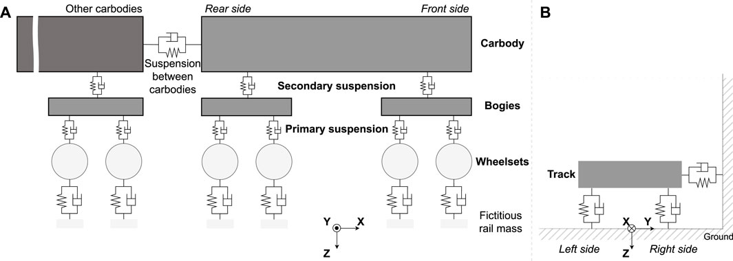
Figure 1. A train-track model: (A) train model in side view and (B) track model in rear view.

Table 1

Table 1. Parameters of the train model.

2.1.2 Track model

As illustrated in Figure 1B, the track mass is connected to the rigid ground through two spring-damper elements. Furthermore, the track mass is laterally attached to a rigid wall via a spring-damper element. Except for vertical translation, the track masses are constrained in all directions.

The selected switch profile is a 60E1-760-1:15 turnout without rail inclination. It has a nominal rail profile of 60E1, a curve radius of 760 m, and a turnout angle of 15°. The switch part in this turnout is represented by ten rail position profiles without any crossing part. The total length of the turnout model is 90 m, with the first 30 m representing a straight track designed to dampen the initial transient effect, and the remaining length representing the turnout model. As illustrated in Figure 2A, the left rail exhibits various profiles in these ten positions (marked with s1—s10 as dotted lines), while the right rail maintains the standard EI60 profile from start to end. Figures 2B,C display the left rail profiles aligned with the left stock rail for these sections. Particularly, the right part of the last position, s10 (cyan), is exactly the same as the profile in s1 (blue). The rail section is defined as the rail part between any two neighbouring positions, having the same profiles in the first positions. Therefore, the nine sections among the ten positions are called s1-s9 in the subsequent parts of the paper, using the names of their start positions.

Figure 2

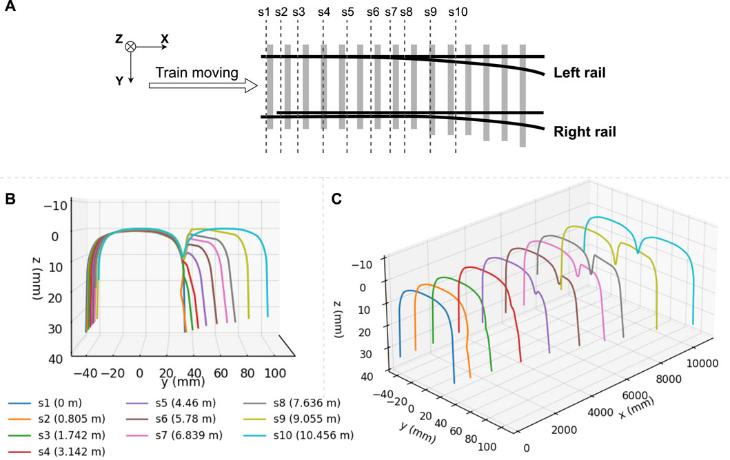
Figure 2. Switch profiles of R760 1:15 turnout: (A) top view, (B) rear view (including ten left rails positions with marked X locations), (C) 45-degree side view.

2.1.3 Wheel—rail contact

The wheel-rail modelling process involves three key stages: creating a geometric model, computing a normal force model, and determining tangential forces (Wu et al., 2020). Two-point contact situations are common due to the geometry of the rail profiles and large lateral wheel displacements. Kassa et al., 2006 describe how two-point contact is simulated and modelled in multibody simulation software like GENSYS. Because of the continuous variation in the shape of the rail cross-section, two-point contact may occur with one point of contact on the stock rail and the other on the switch rail. Figure 3 illustrates a wheel-rail model with two contact points on the left side (cp1 on the tread side and cp2 on the flange side) and only cp1 contact on the right side. The Hertz contact was utilized to compute the normal force, and the tangential forces were calculated using the FASTSIM algorithm. In GENSYS, KPF is a function used to generate a lookup table based on provided wheel and rail profiles. Wheel-rail forces are calculated through interpolation in this table, defined as function Creep_lookuptable_1. To address the diverse rail section profiles along the switches, the built in function Wr_coupl_pe4 was applied. Additional information about wheel-rail modelling can be found in the GENSYS user manual (Persson, 2023). The wheelset profile in the experiment is ENS1002t32.5.

Figure 3

Figure 3. A wheel—rail modelling with three contact points.

2.2 Wear model

There is limited literature on the evolution of rail profiles for railway turnouts, particularly concerning the wear of switches. In this work, an approximate function is utilized to simulate wear referring to the 20 Mt (total tonnage burden) output of the experimental results (Xu et al., 2018). The assumption is that rail wear occurs primarily in the sliding zone, and wear simulation relies on Archard’s wear law. According to this law, the simulated wear depth is directly proportional to the wear coefficient, normal stresses, and relative slide displacement, and inversely proportional to the material hardness (Xu et al., 2018). To assess the correlation between the degree of rail wear and optimal accelerometer placement, nine groups of wear development curves (wear1-wear9) were used in the experiment for all switch profile sections. Figure 4 shows five representative sections. The first two groups of figure are the left and right rail profiles in position s1. The position s4 includes the likely start of two-point contact. From s7, the flange contact had much wear and dominated the wear development until s9. The wear9 curve referred to 20 Mt condition and the rest are linearly interpolated with zero value, indicating unworn rails (wear0). The grinding operation is simulated to remove a 3 mm depth of steel from the rail, adhering to Bane NOR’s regulations. This process ensures the rails can ideally recover their original profiles.

Figure 4

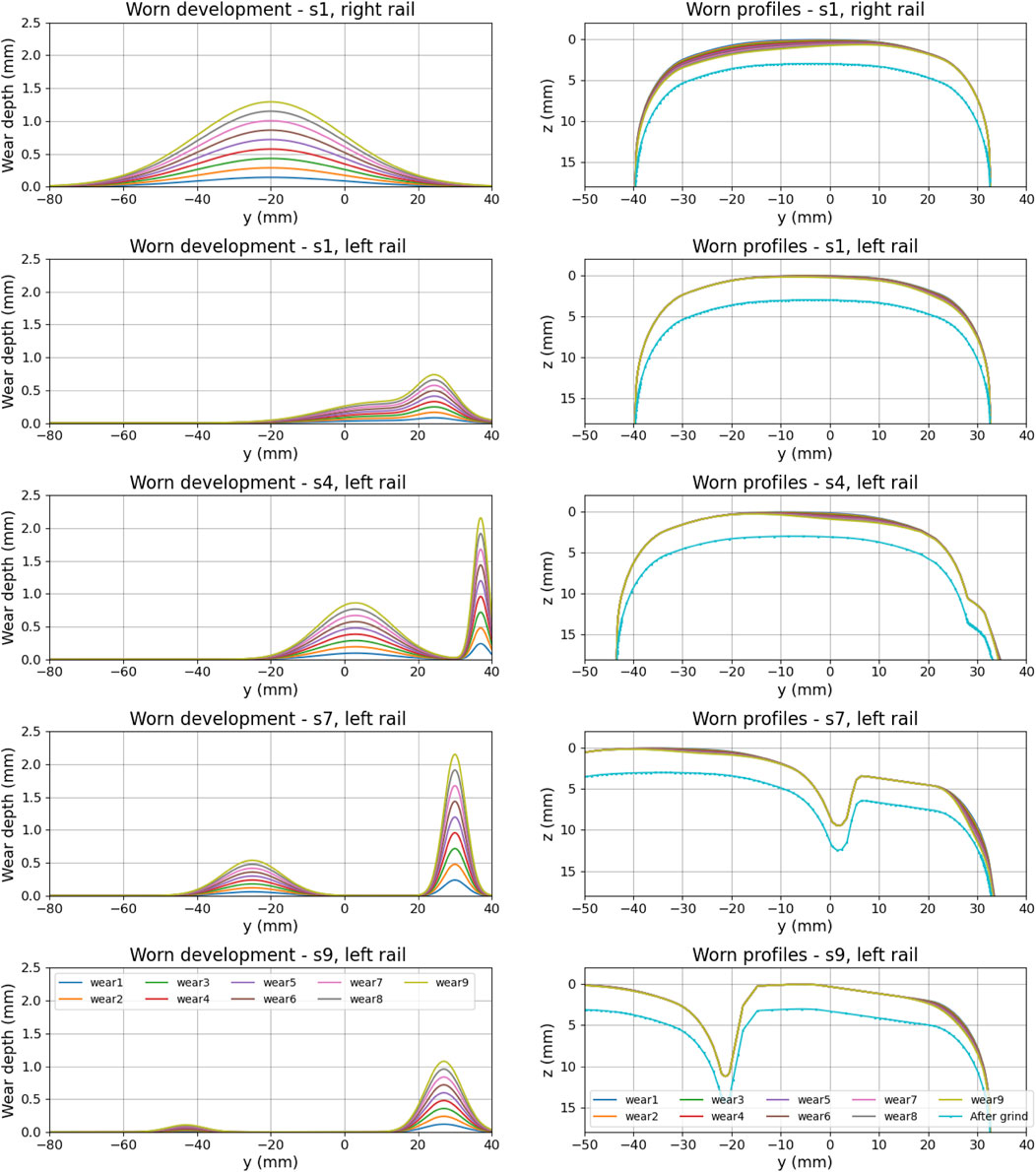
Figure 4. The wear simulation curves and corresponding worn rail profiles in several typical sections (s1, s4, s7, s9).

2.3 Analysis

The goal is to identify the optimal installation locations for accelerometers on trains to achieve the highest sensitivity correlation between acceleration and wear conditions. It means that placing sensors in these locations facilitates easier and more accurate wear detection. After comparing the results of selecting sensor locations in the first carriage and the other three carriages, it was observed that the accelerations in the latter were more damped out due to increased couplings constrained and affected between sensor locations and wheel-rail contact points. Consequently, the decision was to install all acceleration sensors only in the first carriage for the experiments, as illustrated in Figure 5. The naming convention follows the pattern ObjectNumXYZ (for example, bog_1_121 represents the longitudinal front, lateral centre and vertical bottom location in the first bogie). There are 93 locations, comprising 5 × 3 × 3 = 45 (car_1_111-car_1_533) for the carbody, 2x3x3x2 = 36 (bog_1_111-bog_2_332) for the bogies, and 4x1x3x1 = 12 (axl_11_111-axl_22_131) for the wheelsets.

Figure 5

Figure 5. The installation locations of accelerometers: (A) 3D view, (B) front view, (C) side view, (D) top view.

The frequency domain results show no distinct peak frequencies beyond 1 kHz, even with a sample rate set at 20 kHz. To capture any peak frequencies within 1 kHz, the sample rate was adjusted to 2 kHz. The primary frequency (f_p) is defined as the frequency with the highest peak. The optimal installation location of accelerometers must not affect f_p in the presence of worn conditions, making them easier to detect in the frequency domain. In addition, the identification of histograms was utilized to assess whether distribution features were impacted.

Wear development occurred simultaneously along the entire switch sections in this research. Pearson’s linear correlation coefficient (P_corr) is selected as the cross-correlation function to measure the correlation between acceleration signals under varying worn conditions on rails and those under unworn conditions. The resulting value falls within the range [−1, 1], where 1 indicates perfect correlation and −1 indicates perfect anti-correlation. The computation between two acceleration signals X and Y is defined as Eq. 1,

$P_{\mathit{corr}}\left(X,Y\right)=\frac{cov\left(X,Y\right)}{\sqrt{D_X}\sqrt{D_Y}}=\frac{{\sum }_n^{i=1}\left(x_i-\bar{x}\right)\left(y_i-\bar{y}\right)}{\sqrt{{\sum }_n^{i=1}{\left(x_i-\bar{x}\right)}^2}\sqrt{{\sum }_n^{i=1}{\left(y_i-\bar{y}\right)}^2}}(1)$

where cov (X,Y) is the covariance of X and Y; $\bar{x}$ and $\bar{y}$ are the mean values respectively; D_X and D_Y are the variances. A value of zero indicates completely no correlation, meaning that a significant change in the acceleration signal is likely due to wear, making it easier to detect. Three-level guidelines for the correlation strength analysis (Liu and Markine, 2019) are used. The levels are weak (∣P_corr∣ < 0.2), moderate (0.2 ≤ ∣P_corr∣ < 0.5) and strong (0.5 ≤ ∣P_corr∣ < 1)

Our research addressed the quantitative assessment of the correlation between the sensitivity of acceleration signals and sensor placement. The acceleration signals are in the vertical direction only, as the longitudinal and lateral directions are not significant for the carbody and bogies. Conversely, the results for the wheelsets in these two directions exhibit similarity in vertical accelerations, with no discernible difference in the installed locations of one wheelset. To organize the analysis efficiently, a pipeline of the analysis process is designed as Figure 6. The installation locations of accelerometer sensors, wheel profiles, and unworn section profiles are prepared before processing. The first step involves producing the required rail profiles based on the given wear degree. The worn rail profiles are then used to perform wheel-rail geometry computation (KPF) and time simulations (TSIM), implemented using GENSYS. The sensitivity analysis covers three types of installed targets: wheelsets, bogies, and carbody. The final placement suggestions for accelerometers are made in all optional installation locations considering the x, y, and z directions in comparison with the unworn case. The sensitivity indicators include P_corr, histograms, and signal features in the time domain, as well as f_p after FFT. An optimal installation location should have lower P_corr values, indicating a low correlation with its unworn counterpart in the time domain. Conversely, it should retain significant f_p values in worn cases. The grind case is covered in the discussion section, as it closely resembles the unworn case.

Figure 6

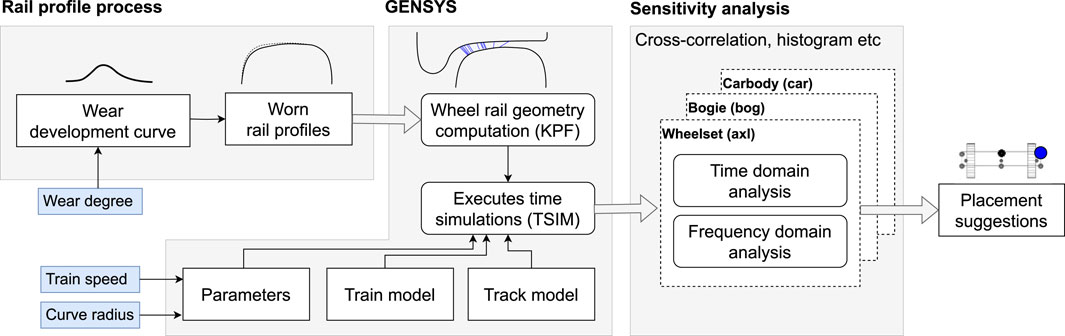
Figure 6. The pipeline of analysis process.

3 Results

3.1 Unworn rails

3.1.1 Wheelsets

The wheelsets, being the bodies closest to the source of vibration from the wheel and rail contact, play a crucial role. The first wheelset (ax11) encounters the vibration source initially along the driving direction in the time domain. In Figure 7, the distance (x-axis) represents how far the train has travelled past the switches, indicating the longitudinal distance between the wheel-rail contact point and the front of the switches in the time domain. The frequency curve (s9) illustrates that ax11 preserves more primary frequencies with varying amplitudes, such as f_p1 (108.02 Hz) and f_p2 (121.53 Hz). These frequency values match the wavelength (0.09 m) inspected in the s9 section figure. The s9 section constitutes the primary contribution of f_p (120.93 Hz) within the entire switch part, surpassing other sections. As a result of the train suspension system’s influence, the remaining three wheelsets consistently exhibit lower amplitudes, particularly in the value ranges near f_p. The wheelsets (ax21 and ax22) in the second bogie introduce additional effects in the 200–400 Hz range, causing a shift in the primary frequencies to 160 Hz as observed. The observed shift may result from the forced vibrations of the train components, characterized by higher frequencies induced by the movement of the first bogie. In other words, the contamination of excited vibrations from other components complicates the identification of the frequency component associated with the passage of the switch. Consequently, in the frequency domain, The first wheelset is recommended for the optimal location, while the least favourable choice is the last one. On the other hand, ax11 exhibits a larger amplitude than the other three and occurs in more sections, for example, s4, s7, s8, and s9. Ax22 covers the least number of sections with vibration, specifically, s8 and s9, while ax12 shows a poor response in s9. From a time-domain perspective, ax12 and ax21 emerge as the better choices. In summary, ax11 is undoubtedly the first choice, and ax21 could be considered for installation if the budget allows.

Figure 7

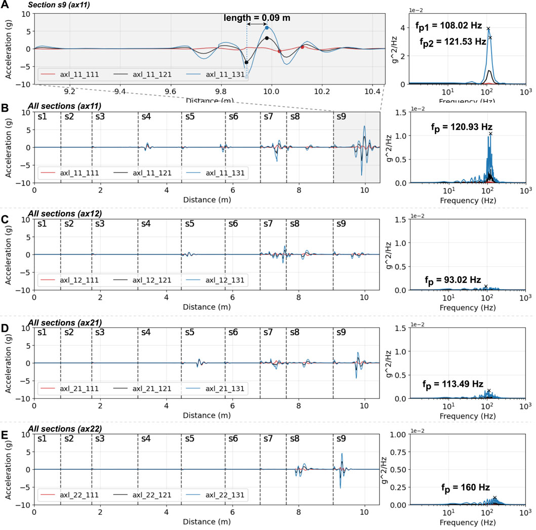
Figure 7. Accelerations and response spectra of wheelsets: (A) ax11, s9, (B) ax11, (C) ax12, (D) ax21, (E) ax 22.

Among these axles, the lateral left (highlighted in blue) has the largest amplitude because it is the closest to the left rail, with more changed sections. The lateral right one (red) exhibits opposite values due to the reaction force of the rigid wheelsets, while the lateral centre location (black) has the minimum amplitude. In the frequency domain, the lateral centre location performs better than the lateral right. These characteristics are more pronounced in the first wheelset. In this case, the lateral left emerges as the most sensitive location. Conversely, the lateral right becomes the most sensitive if there are significant changes in the switch rails on the right. In real-world scenarios, an alternative approach to measuring acceleration along the lateral direction is to install sensors on both sides. This allows the calculation of values for the remaining positions through interpolation, aiding in the differentiation of sensitivity on the left or right rails.

3.1.2 Bogies

In the vertical direction (z), there is very little difference observed when sensors are installed at the bottom and top of the bogies. Positions at the vertical bottom are chosen to compare results along the longitudinal direction (x) for two bogies, as illustrated in Figure 8. The black vertical cross marks the primary frequency f_p found in wheelsets, which would like to be found. All the figures show large values in the low-frequency range of 0–100 Hz. However, the worst cases are observed when installed on bogie2, where amplitudes in the low frequency exceed even the primary frequency. This makes it challenging to distinguish the primary frequency if it falls within the same range. Conversely, the lateral center exhibits the smallest amplitude but a clear frequency distribution.

Figure 8

Figure 8. Accelerations and response spectra of bogies: (A) bogie1, lateral right, s9, (B) bogie1, lateral right, (C) bogie1, lateral center, (D) bogie1, lateral left, (E) bogie2, lateral right, (F) bogie2, lateral center, (G) bogie2, lateral left.

The rear locations of bogie (bog_1_311 and bog_2_311, highlighted in blue) perform the best longitudinally for lateral right, while the front locations (bog_1_121 and bog_1_131, in red) are relatively better in the other figures. Considering the worse performance of the installation on bogie2, the installation locations bog_1_131, bog_1_121, and bog_1_311 are the top three choices, maintaining larger values in sensitive sections s9, s7, s8, s4, and s5.

3.1.3 Carbody

The three optional vertical locations (floor, center, and ceiling) yield nearly identical results to the bogies, making vertical floor locations suitable representatives. The maximum amplitude in the time domain is very small, approximately 0.015 g, due to the benefits of the suspension system. In addition, only low-frequency values can be captured, implying a limited chance of capturing any higher frequency than 70 Hz, such as the primary frequency f_p of ax11. This is because the suspension system has a much larger effect, especially lower than 70 Hz, compared to the bogies. Therefore, a 4th-order Butterworth high-pass 70 Hz filter was applied to all carbody accelerometers to ensure that the accelerations could be analyzed. Despite this, the maximum amplitude of filtered acceleration decreased to lower than 0.001 g. Both Figures 9A,B exhibit similar features in the time and frequency domains, indicating that the carbody was triggered to vibrate when the first bogie (ax11) and the second bogie (ax21) reached switch positions. It is noted that Figure 9B has only 1/10 amplitude compared to Figure 9A. To minimize the influence of the suspension system, the switch positions when the first bogie reaches should be used as the reference for further discussion since the suspension system has less impact on the acceleration values. The intermediate locations (highlighted in pink and green) in the longitudinal direction can be represented by the maximum locations (red and blue) respectively. In this case, the installation locations car_1_131 and car_1_121 are the best choices, showing noticeable accelerations in sensitive sections s9, s7, s4, s8, and s5.

Figure 9

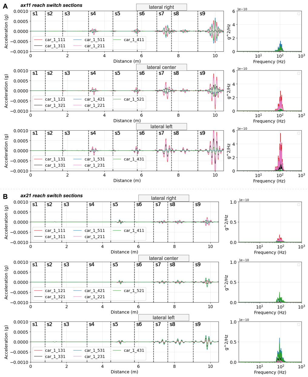
Figure 9. Accelerations and response spectra of the carbody: (A) the first bogie (ax11) reached switch sections and (B) the second bogie (ax21) reached switch sections.

3.2 Worn rails

3.2.1 Wheelsets

Utilizing the Pearson correlation (P_corr) heatmap presented in Figure 10, it is observed that correlation values decrease rapidly after the initial two or three rounds of wear in the time domain. In comparison to the range of the heatmap scale in the time domain, the values in the frequency domain exhibit more stable patterns ranging from 0.65 to 0.93, indicating more consistent frequency curves among various worn and unworn conditions. Every set of three consecutive rows exhibits a consistent value pattern as they are positioned in the same longitudinal location. Within each set, the last two rows, situated at the lateral centre and left locations, consistently display closely aligned values in most cases. This aligns with the observations made in the analysis of the unworn case.

Figure 10

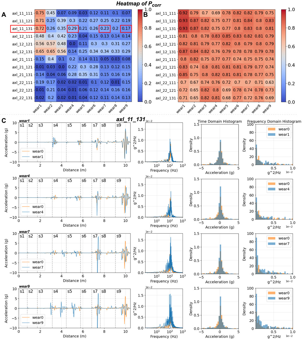
Figure 10. Accelerations and response spectra of wheelsets in worn cases: (A) P_corr heatmap in the time domain, (B) P_corr heatmap in the frequency domain, (C) the accelerations and histograms of axl_11_131 in four wear cases (wear1, wear4, wear7, wear9).

For further analysis, axl_11_131, identified as the optimal location during the assessment of an unworn rail, is chosen to investigate wear1, wear4, wear7, and wear9 cases. This exploration encompasses raw data and histograms in both time and frequency domains. Among these cases, wear1 emerges as the best match due to its minimal wear. Notably, significant differences are observed in specific sections, such as s7 and s5, in the time domain, where high-frequency signals appear to initiate distortion, particularly values exceeding 200 Hz. Although wear7 and wear9 exhibit favourable matching distributions in the histogram, the disparity in time domain values increases substantially from wear7 and peaks in wear9. In summary, while the primary pattern is well-preserved across all wear cases, escalating wear introduces challenges in detecting frequencies exceeding 200 Hz.

3.2.2 Bogies

Figure 11 presents the results on the two bogies using heatmaps of P_corr. Bogie1 exhibits noticeably better sensitivity results, characterized by a wider value range, in comparison to bogie2. In each group along the lateral direction, consisting of three sensors, the first (lateral right) and third sensors (lateral left) consistently display higher values than the second sensor (lateral middle). Additionally, the lateral left positions yield the lowest values. Therefore, bog_1_131 is identified as the ideal location. The signals in the frequency domain exhibit a similar trend to those in the time domain, though not duplicated here.

Figure 11

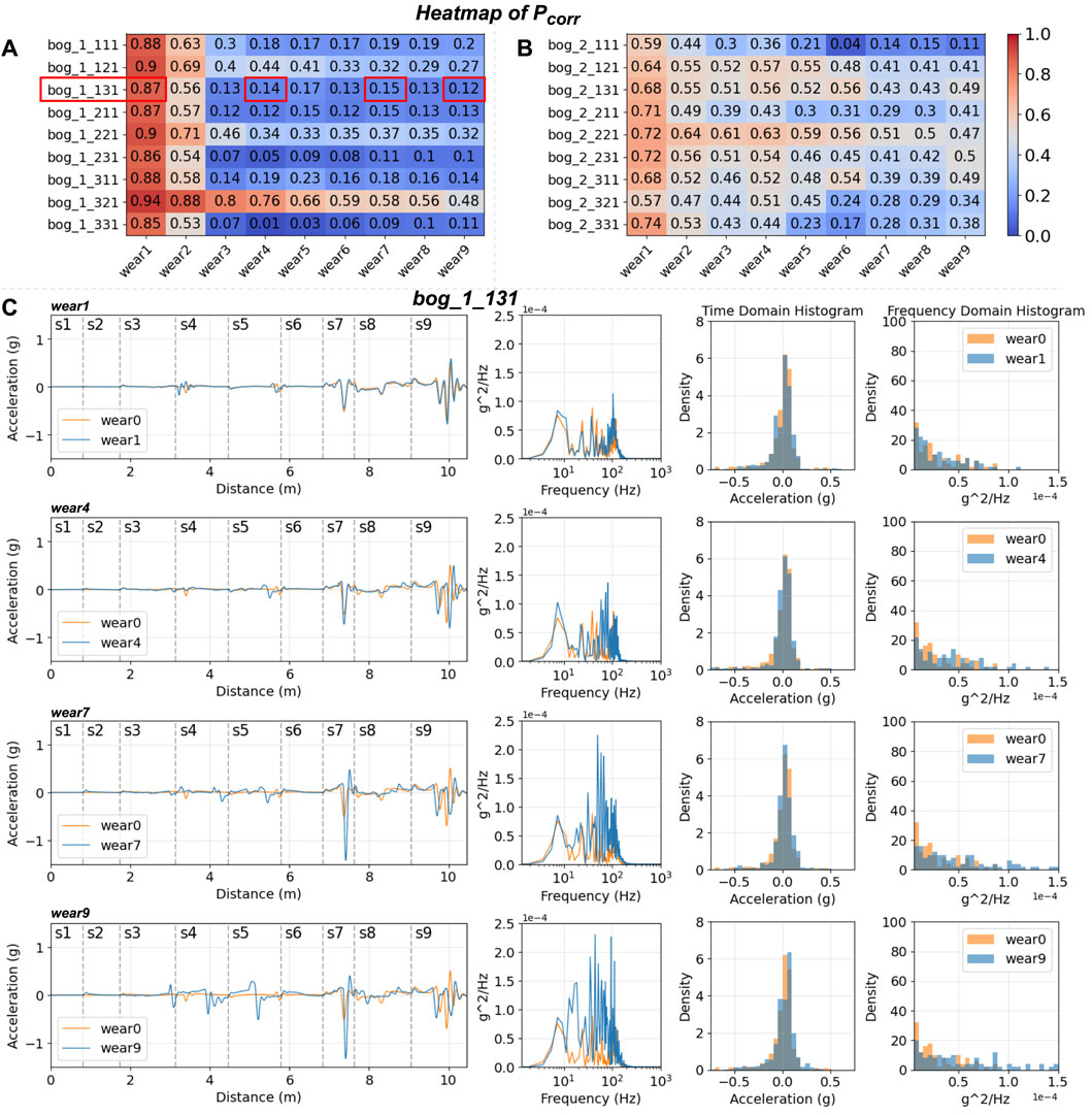
Figure 11. Accelerations and response spectra of bogies in worn cases: (A) P_corr heatmap in the time domain for bogie1, (B) P_corr heatmap in the time domain for bogie2, (C) the accelerations and histograms of bog_1_131 in four wear cases (wear1, wear4, wear7, wear9).

The histograms in both time and frequency domains generally exhibit good alignment, except for values near zero. The suspension system significantly affects the low-frequency values. Compared to the unworn case (orange), a more pronounced distortion in values emerges from wear4 and persists until wear9 in the frequency domain, particularly noticeable in sections s7, s9, s5, and s4 in the time domain.

3.2.3 Carbody

About the sensor locations in the carbody, the positions (car_1_131, car_1_121, car_1_311, and car_1_531) exhibit large value ranges for various wear cases in the P_corr heatmap of Figure 12 in the same longitudinal group. Considering the findings from unworn rail cases, both car_1_131 and car_1_121 are selected for further discussion. Both sensors display similar value patterns throughout the wear development, such as peak values (highlighted in blue) in sections s3, s4, s5, s6, s7, and s9 for wear 9. On the other hand, car_1_121 shows relatively smaller value changes, indicating that some vibration has been damped out, such as in section s7 for wear 7 and 9 cases. Therefore, car_1_131 is superior to any other sensor on the carbody.

Figure 12

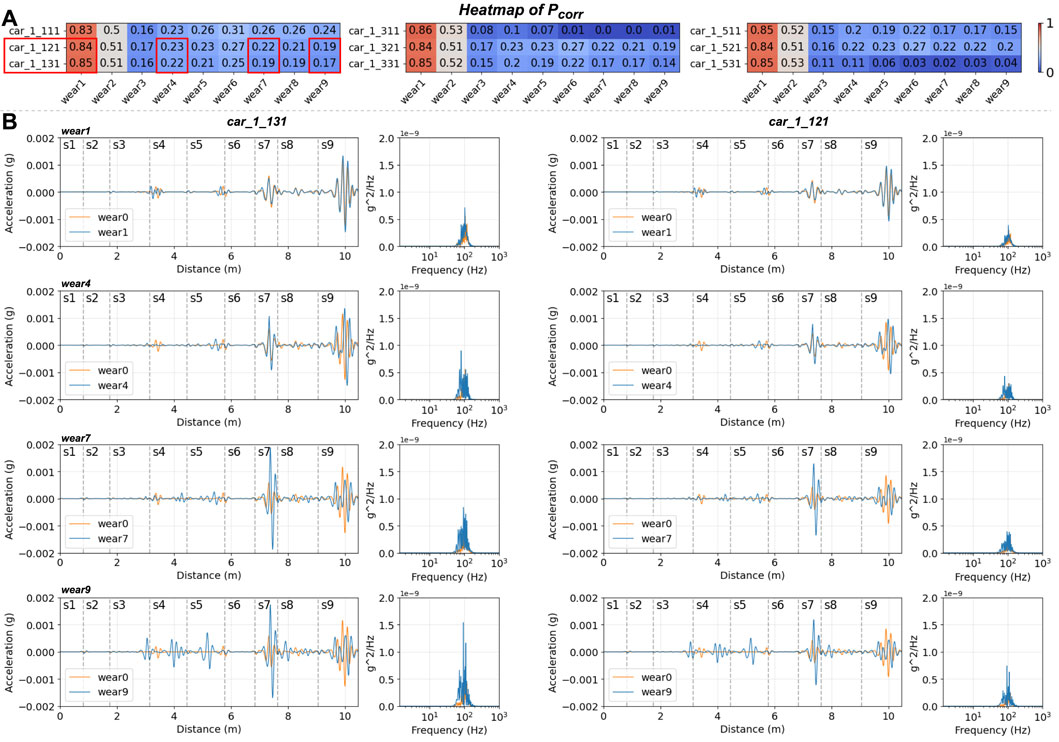
Figure 12. Accelerations and response spectra of the carbody in worn cases: (A) P_corr heatmap in the time domain and (B) the accelerations and histograms of car_1_131 and car_1_121 in four wear cases (wear1, wear4, wear7, wear9).

4 Discussion

4.1 Optimal sensor placement

Three key observations need to be addressed: similarity in the z-axis, better in earlier contact, and the first excitation dominates. Firstly, the vertical location of the same object will almost not affect sensitivity, and the default location can be set to the ones closest to the vibration source, the contact points between wheels and rails. Secondly, installing sensors at the rear is less effective than at the front in the longitudinal direction because more suspension dampens out the vibration signals and adds more low-frequency signals, posing challenges in distinguishing the primary frequency of the wheelset. Meanwhile, the centre of the object is the least favourable location due to less vibration occurring in the centre. Lastly, objects will vibrate upon each time when the various wheelsets encounter switches, with the first wheelset being the most representative. It is attributed to the suspension system’s inability to fully dampen the vibration triggered by external contact forces. This occurs after the first wheelset accesses the switch, and before the subsequent wheelset reaches it. For example, the carbody will experience similar vibration when four wheelsets encounter switches with different time delays. Section 3.1.3 selects two typical cases and demonstrates that the first is the ideal signal to be analyzed.

Figure 13A summarizes the optimal accelerometer placement suggestions based on the evaluation results according to these three conclusions. In the extreme case of a limited budget, the ideal installed position is bog_1_131, using a 2g (19.6 m/s²) accelerometer, commonly found in mobile phones. Secondly, the solution could involve adding sensors on car_1_131, located on the carbody, and on the wheelset location ax_11_131 with a 20g (196 m/s²) range. Additionally, more sensors installed on the same object can capture the distribution of an object. For example, two sensors on the same wheelset can be used to compute for this linear object. Three sensors on the bogie can be used for calculating the acceleration value at any point on the bogie. In the real world, if changes in switch profiles occur evenly on the left and right rails, it is suggested to add two sensors on the left and right instead of the lateral centre.

Figure 13

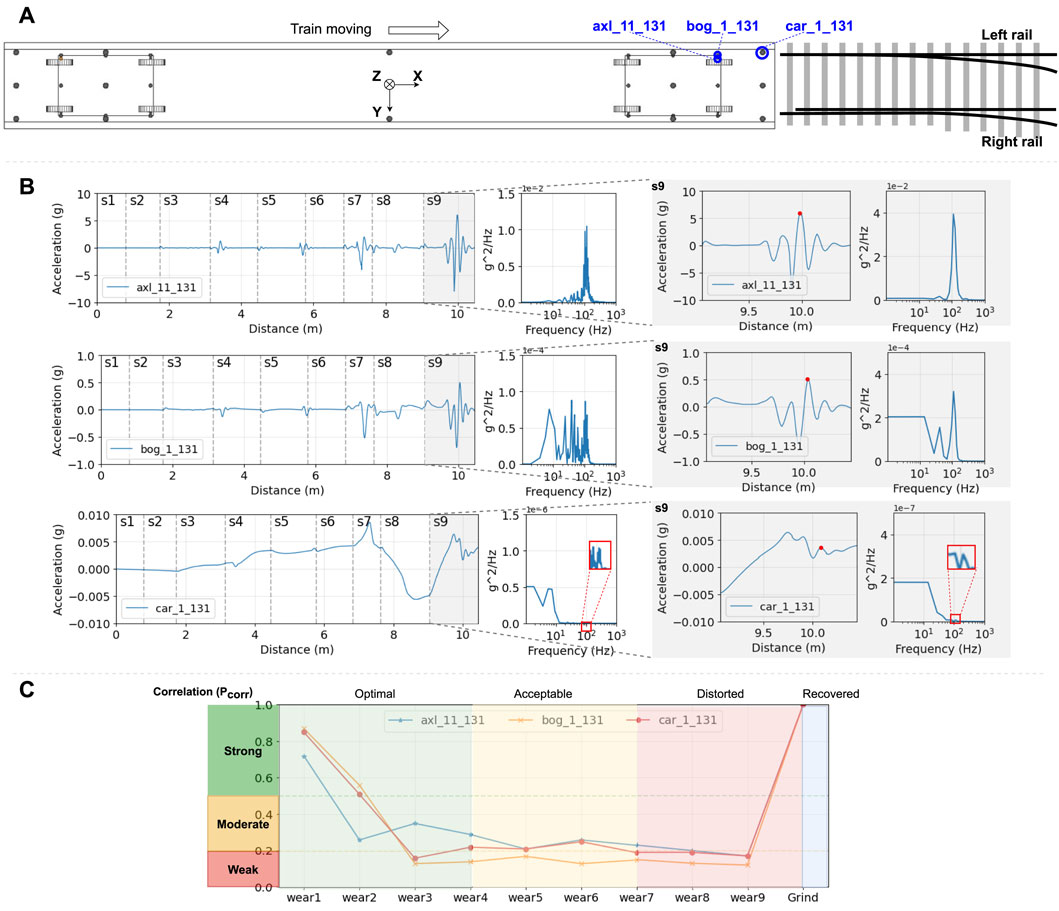
Figure 13. (A) The optimal accelerometer placement suggestions based on experimental data. (B) The correlation between optimal placement on the wheelset, bogie and carbody under unworn cases.(C) Four stages of sensitivity with wear development and correlation levels.

4.2 The correlation between wear and sensitivity of vertical acceleration

Figure 13B show that the acceleration significantly decreases from the wheelset to the carbody with the increasing influence of the suspension system when the rails are unworn. The amplitude ratio is approximately 0.01 g (carbody):1 g (bogie):10 g (wheelset). Comparing the frequency curves, the bogie still retains the primary frequency with a zoomed amplitude in the time domain, and the trends remain consistent. For the carbody, values in the primary frequency are almost diminished even when zoomed in. Analyzing the results in s9, the time delay can be observed by tracking the x-values of red dots, and the patterns in the frequency domain are more apparent. If no filter is used for the carbody accelerometers, the sensor has very little frequency information reserved and is only affected by the large geometry changes of the switch sections. These features persist similarly regardless of how the wear develops. The detectable range of accelerometers is only 0.001 g after using the high-pass filter. It means the accelerometers installed in the carbody can have only 1/10000 sensitivity compared to the wheelset in the simulation. It results in difficulty capturing any pertinent data within this low-frequency range and makes it more susceptible to signal noises in reality. On the other hand, the sensitivity of vertical acceleration can be divided into four stages (optimal, acceptable, distorted and recovered), as Figure 13C illustrates. In the early stage, the wear is very small, and the acceleration signals are very close to the conditions without any wear. When the wear is large enough, the results gradually lose the details in the time domain while still preserving the main frequencies. In the third phase, the signals begin to be disturbed, especially in the frequency domains. It will last to the worst case in wear 9 and recover completely after the grind.

Taking the location axl_11_131 as a case study, the power spectral density (PSD) analysis was conducted, with a focus on the highest PSD value indicative of the primary frequency referred to (Li et al., 2021). In Figure 14A (left), each section is depicted individually, while the data in all sections is represented in grey color. All primary frequencies are denoted by crosses. Sections s1, s2, and s3 exhibit notably lower PSD values and distinct curve shapes compared to the grey curve. Meanwhile, s9 (blue) emerges as the primary contributor, closely mirroring the primary frequency (red cross) observed in the grey curve.

Figure 14

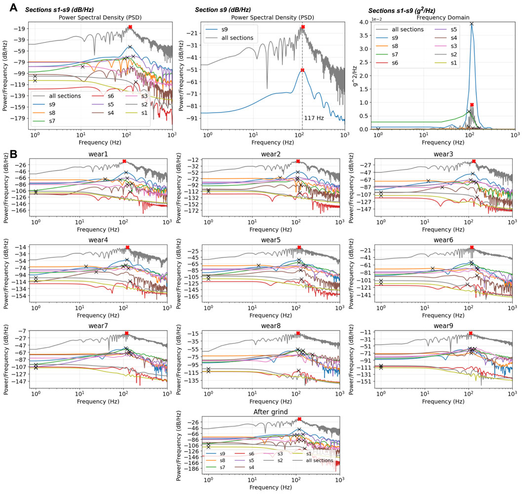
Figure 14. The vertical acceleration of axl_11_131. (A) (left) PSD for each section and all sections, (middle) PSD for s9 and all sections, (right) PSD for each section and all sections with unit g²/Hz. (B) PSD for all sections and separate ones compared with various wear conditions.

Figure 14A (middle) highlighted the primary frequency, revealing a consistent value of 117 Hz across both s9 and all sections’ curves. These curves exhibit a high degree of similarity in their trends. Considering the train speed 70 km/h, the corresponding wavelength of acceleration is determined to be 168 mm. For amplitude analysis, following established literature conventions (Böröcz and Singh, 2017; Sun et al., 2021), the unit g²/Hz is utilized in Figure 14A (right). The top two contributing sections to the amplitude are identified as s7 and s9, particularly in the proximity of the primary frequency. Consequently, the unit g²/Hz is used in the rest of this paper for better understanding. Figure 14B illustrates that the sensitive regions can be found in terms of PSD. From wear1 to wear4, the S9 (blue) dominates the trend, exhibiting the highest values (marked with crosses) compared to the grey curve (representing all sections). However, the S7 (green) and other sensitive sections gradually influence the grey curve, reaching their maximum impact in wear9. Eventually, it returns to a status close to the unworn case after the grinding of the rail. This disturbance is more severe when the geometry sections are sensitive, for example, s4, s5, s7, s8, and s9.

4.3 Various train speeds and curve radii

The train speed (70 km/h) and curve radius (760 m) were used in the previous experiments. Before deciding on this configuration, variations in train speeds and curve radii were explored. For instance, the train speed varies from 50 km/h to 80 km/h with different curve radii (300 m, 500 m, 760 m, 1200 m, 2500 m) according to Bane NOR regulations. Figure 15A illustrates the values of accelerometer axl_11_131 in the vertical direction for various train speeds under a 760 m curve radius after aligning them with the distance to the start of switches. In the time domain, the amplitude decreases with the decreasing train speed because the slower speed results in softer wheel-rail contacts with less force magnitudes. The lower train speed leads to an earlier completion of the damping period when forces and accelerations are higher, such as in sections s7 and s9. They show a higher and more significant influence for all sections in the frequency domains. Figure 15B presents the results for different curve radii assuming the train speed is set to 70 km/h. The results for R760, R1200, and R2500 show a similar trend in the time domain and very close features in the frequency domain. However, excessively tight curves, such as R500 (orange) and R300 (red), show larger amplitudes and messier frequency results, and the train speed is not allowed to be set as high as 70 km/h in reality. In summary, a radius of R760 and a train speed of 70 km/h can be considered representative of most cases.

Figure 15

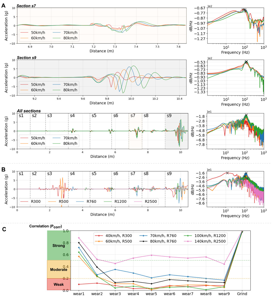
Figure 15. The vertical acceleration of axl_11_131. (A) At the curve radius of 760 m, the train speeds of 80, 70, 60, and 50 km/h are considered. (B) The train speed is 70 km/h at curve radii of 300, 500, 760, 1200, and 2500 m. (C) P_corr in various worn scenarios for six typical cases.

There are six typical cases designed to illustrate worn scenarios in Figure 15C. The results show that a tight curve case (red) exhibits a very weak correlation from the early wear stage and minimal value changes during wear development. This makes it easier to detect the existence of wear but poses a high challenge in evaluating the degree of wear development. In contrast, a case with a more straight line (pink) shows a relatively strong correlation, making it difficult to distinguish whether wear has occurred. Therefore, the case of 70 km/h, R760 (blue), is more representative for discussion as it reflects the four stages of the entire process, as shown in Figure 13C.

4.4 Limitations

In this paper, the number of switch sections is limited to ten, and the minimum interval distance is 0.797 m, occurring between s7 and s8. Although the simulation uses a sample rate of 2 k Hz or even higher, the larger interval value causes the simulation to be less sensitive than the real world. The profiles of switch sections with small intervals are challenging to measure, especially the wear development over time. One approach to overcome this limitation is to utilize MiniProf or 3D scanner technology for efficient and precise measurement. It can be utilized to precisely investigate the correlation between accelerations and track irregularities, a topic not addressed in this paper. In addition, the discussion of experimental results focuses on the vertical acceleration for a representative case with a radius of R760 and a train speed of 70 km/h. Train speeds below 50 km/h and tight curves, such as those with radii of 300 m and 500 m, are not recommended for analysis using our approach.

5 Conclusion

This paper utilized the multibody simulation software GENSYS to simulate a train passing through a railway switch under diverse wear conditions. The vertical accelerations generated by accelerometers on the train were used to determine the optimal placement of these sensors, namely, by using time and frequency domain analyses. Under various worn conditions, the discussion emphasizes the sensitive sections within the unworn cases. The present study’s outcomes are summarized in these conclusions.

• It is suggested that the placement is to prioritize installing sensors on the first bogie, positioned on top of the rail side close to the wheel-rail contact points. Through our analysis, three main key observations were identified: maintaining similarity along the z-axis, favoring the earlier contact position in the x-axis, and acknowledging the dominance of the first excitation.

• The correlation between wear and vertical acceleration, extending from wheelsets to the carbody, indicates that sensitivity experiences four stages: optimal, acceptable, distorted, and recovered. The measurement range ratio is 10:1:0.01 (wheelset:bogie:carbody). It is noted to employ a high-pass filter to obtain relevant acceleration data if accelerometers are installed in the carbody to detect wear conditions.

• The case, with a curve radius of R760 and a train speed of 70 km/h, is considered representative after analyzing various scenarios.

These results provide the scientific support of placing accelerometers in more effective and sensitive locations, selecting reasonable measurement ranges and analyzing the most valuable collected data. Although the magnitudes of accelerations in the carbody are significantly lower than those on wheelsets, it demonstrates the potential for installing accelerometers in the carbody considering the similar correlation between wear development and acceleration for wheelsets, bogies, and carbody. The feasibility of installation and maintenance makes it highly promising. The direct correlation between the depth of switch wear and the magnitude of acceleration provides an opportunity to detect switch wear more effectively in its early stages, thereby indicating the appropriate time for grinding operations. If accelerometers were installed in optimal locations on trains and configured with thresholds for monitoring wear conditions, they could assist decision-makers in optimizing maintenance routines for switches, thus improving safety and efficiency in railway operations.

Data availability statement

The technical data of the train model are not publicly available due to commercial reasons. The other raw data supporting the conclusion of this article will be made available by the authors, without undue reservation.

Author contributions

ZH: Writing–original draft, Writing–review and editing. AL: Writing–original draft, Writing–review and editing. JD: Writing–original draft, Writing–review and editing. GF: Writing–original draft, Writing–review and editing.

Funding

The author(s) declare that no financial support was received for the research, authorship, and/or publication of this article.

Conflict of interest

The authors declare that the research was conducted in the absence of any commercial or financial relationships that could be construed as a potential conflict of interest.

Publisher’s note

All claims expressed in this article are solely those of the authors and do not necessarily represent those of their affiliated organizations, or those of the publisher, the editors and the reviewers. Any product that may be evaluated in this article, or claim that may be made by its manufacturer, is not guaranteed or endorsed by the publisher.

References

Aminullah, A., Suhendro, B., and Panuntun, R. B. (2020). “Optimal sensor placement for accelerometer in single-pylon cable-stayed bridge,” in International conference on sustainable civil engineering structures and construction materials (Springer), 63–79. doi:10.1007/978-981-16-7924-7_5

CrossRef Full Text | Google Scholar

Artagan, S. S., Bianchini Ciampoli, L., D’Amico, F., Calvi, A., and Tosti, F. (2020). Non-destructive assessment and health monitoring of railway infrastructures. Surv. Geophys. 41, 447–483. doi:10.1007/s10712-019-09544-w

CrossRef Full Text | Google Scholar

Barkhordari, P., Galeazzi, R., and Blanke, M. (2020). Prognosis of railway ballast degradation for turnouts using track-side accelerations. Proc. Institution Mech. Eng. Part O J. Risk Reliab. 234, 601–610. doi:10.1177/1748006X20901410

CrossRef Full Text | Google Scholar

Böröcz, P., and Singh, S. P. (2017). Measurement and analysis of vibration levels in rail transport in central europe. Packag. Technol. Sci. 30, 361–371. doi:10.1002/pts.2225

CrossRef Full Text | Google Scholar

Castillo-Mingorance, J. M., Sol-Sánchez, M., Moreno-Navarro, F., and Rubio-Gámez, M. C. (2020). A critical review of sensors for the continuous monitoring of smart and sustainable railway infrastructures. Sustainability 12, 9428. doi:10.3390/su12229428

CrossRef Full Text | Google Scholar

Chudzikiewicz, A., Bogacz, R., and Kostrzewski, M. (2014). “Using acceleration signals recorded on a railway vehicle wheelsets for rail track condition monitoring,” in EWSHM-7th European workshop on structural health monitoring (La Cité, Nantes, France: EWSHM).

Google Scholar

Cornish, A., Smith, R. A., and Dear, J. (2016). Monitoring of strain of in-service railway switch rails through field experimentation. Proc. Institution Mech. Eng. Part F J. Rail Rapid Transit 230, 1429–1439. doi:10.1177/0954409715624723

CrossRef Full Text | Google Scholar

Dižo, J., Blatnickỳ, M., Gerlici, J., Leitner, B., Melnik, R., Semenov, S., et al. (2021). Evaluation of ride comfort in a railway passenger car depending on a change of suspension parameters. Sensors 21, 8138. doi:10.3390/s21238138

PubMed Abstract | CrossRef Full Text | Google Scholar

Dumitriu, M. (2019). Fault detection of damper in railway vehicle suspension based on the cross-correlation analysis of bogie accelerations. Mech. Industry 20, 102. doi:10.1051/meca/2018051

CrossRef Full Text | Google Scholar

Eiken, A. W. (2022) “Position alignment and geographical location determination of railway track condition monitoring data,”. Master’s thesis. Trondheim, Norway: NTNU.

Google Scholar

Fernández-Bobadilla, H. A., and Martin, U. (2023). Modern tendencies in vehicle-based condition monitoring of the railway track. IEEE Trans. Instrum. Meas. 72, 1–44. doi:10.1109/TIM.2023.3243673

PubMed Abstract | CrossRef Full Text | Google Scholar

International Transport Forum, O. (2024). Rail infrastructure maintenance spending.

Google Scholar

Jiang, T., Frøseth, G. T., and Rønnquist, A. (2023). A robust bridge rivet identification method using deep learning and computer vision. Eng. Struct. 283, 115809. doi:10.1016/j.engstruct.2023.115809

CrossRef Full Text | Google Scholar

Kassa, E., Andersson, C., and Nielsen, J. C. (2006). Simulation of dynamic interaction between train and railway turnout. Veh. Syst. Dyn. 44, 247–258. doi:10.1080/00423110500233487

CrossRef Full Text | Google Scholar

Lei, S., Ge, Y., and Li, Q. (2020). Effect and its mechanism of spatial coherence of track irregularity on dynamic responses of railway vehicles. Mech. Syst. Signal Process. 145, 106957. doi:10.1016/j.ymssp.2020.106957

CrossRef Full Text | Google Scholar

Li, J., Wang, Q., and Chen, X. (2021). “Analysis of rail corrugation characteristics based on PSD,” in International Conference on Smart Transportation and City Engineering 2021 (Society of Photo-Optical Instrumentation Engineers (SPIE)), 1027–1039. doi:10.1117/12.2613909

CrossRef Full Text | Google Scholar

Liu, X., and Markine, V. L. (2019). Correlation analysis and verification of railway crossing condition monitoring. Sensors 19, 4175. doi:10.3390/s19194175

PubMed Abstract | CrossRef Full Text | Google Scholar

Mahjoubi, S., Barhemat, R., and Bao, Y. (2020). Optimal placement of triaxial accelerometers using hypotrochoid spiral optimization algorithm for automated monitoring of high-rise buildings. Automation Constr. 118, 103273. doi:10.1016/j.autcon.2020.103273

CrossRef Full Text | Google Scholar

Malekjafarian, A., Obrien, E. J., Quirke, P., Cantero, D., and Golpayegani, F. (2021). Railway track loss-of-stiffness detection using bogie filtered displacement data measured on a passing train. Infrastructures 6, 93. doi:10.3390/infrastructures6060093

CrossRef Full Text | Google Scholar

Malekjafarian, A., Sarrabezolles, C.-A., Khan, M. A., and Golpayegani, F. (2023). A machine-learning-based approach for railway track monitoring using acceleration measured on an in-service train. Sensors 23, 7568. doi:10.3390/s23177568

PubMed Abstract | CrossRef Full Text | Google Scholar

Nieminen, V., and Sopanen, J. (2023). Optimal sensor placement of triaxial accelerometers for modal expansion. Mech. Syst. Signal Process. 184, 109581. doi:10.1016/j.ymssp.2022.109581

CrossRef Full Text | Google Scholar

Papadimitriou, C. (2004). Optimal sensor placement methodology for parametric identification of structural systems. J. sound Vib. 278, 923–947. doi:10.1016/j.jsv.2003.10.063

CrossRef Full Text | Google Scholar

Persson, I. (2023). Gensys manual.

Google Scholar

Rahimi, M., Liu, H., Cardenas, I. D., Starr, A., Hall, A., and Anderson, R. (2022). A review on technologies for localisation and navigation in autonomous railway maintenance systems. Sensors 22, 4185. doi:10.3390/s22114185

PubMed Abstract | CrossRef Full Text | Google Scholar

Sun, Q., Chen, C., Kemp, A. H., and Brooks, P. (2021). An on-board detection framework for polygon wear of railway wheel based on vibration acceleration of axle-box. Mech. Syst. Signal Process. 153, 107540. doi:10.1016/j.ymssp.2020.107540

CrossRef Full Text | Google Scholar

Usoro, A. E. (2015). Some basic properties of cross-correlation functions of n-dimensional vector time series. J. Stat. Econ. Methods 4, 63–71.

Google Scholar

Worden, K., and Burrows, A. (2001). Optimal sensor placement for fault detection. Eng. Struct. 23, 885–901. doi:10.1016/S0141-0296(00)00118-8

CrossRef Full Text | Google Scholar

Wu, Q., Spiryagin, M., Persson, I., Bosomworth, C., and Cole, C. (2020). Parallel computing of wheel-rail contact. Proc. Institution Mech. Eng. Part F J. Rail Rapid Transit 234, 1109–1116. doi:10.1177/0954409719880737

CrossRef Full Text | Google Scholar

Xu, J., Wang, P., Wang, J., An, B., and Chen, R. (2018). Numerical analysis of the effect of track parameters on the wear of turnout rails in high-speed railways. Proc. Institution Mech. Eng. Part F J. Rail Rapid Transit 232, 709–721. doi:10.1177/0954409716685188

CrossRef Full Text | Google Scholar

Zhang, C., Shen, S., Huang, H., and Wang, L. (2021). Estimation of the vehicle speed using cross-correlation algorithms and mems wireless sensors. Sensors 21, 1721. doi:10.3390/s21051721

PubMed Abstract | CrossRef Full Text | Google Scholar

Zwanenburg, W. J. (2009) Modelling degradation processes of switches and crossings for maintenance and renewal planning on the Swiss railway network. Lausanne: Tech. rep., EPFL. doi:10.5075/epfl-thesis-4176

CrossRef Full Text | Google Scholar