Amodal completion of coincidentally occluded angles: a matter of visual approximation

1. Introduction

Years ago, Gerbino (1978) discussed a perceived distortion observed in displays such as those in Figures 1B–D, where angles of a partially occluded polygon are coincidentally occluded.¹ Such displays are characterized by perpendicular T-junctions between the occluding edge and the angle's sides, so ruling out the regression to right-angles tendency often invoked to explain the misalignment observed in classic displays with non-perpendicular T-junctions, like the Poggendorff illusion (Hotopf et al., 1974).

FIGURE 1

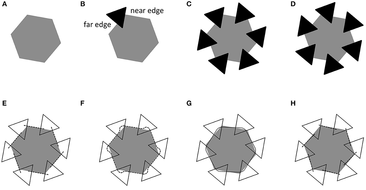
Figure 1. The Gerbino illusion. A distortion is perceived when an angle of the regular hexagon in (A) is coincidentally occluded as in (B). The distortion is more salient when all angles are coincidentally occluded [see (C) for CCW occlusion and (D) for CW occlusion]. Within the visual interpolation framework, the perceived distortion might reflect the amodal continuation of T-stems behind occluding triangles (E) or the possible interpolation of smooth yet non-monotonic amodal contours (F). Within the visual approximation framework, the hexagon might be completed by a smooth monotonic amodal contour if the orientation of the sides of the hexagon is misrepresented [like in (G) for the CCW pattern in (C)]. Such internal representation might conflict with sensory evidence and underlie the opposite perceived misorientation shown in (H).

As shown in Figure 1B a distortion is perceived even when a single angle of a regular hexagon is coincidentally occluded; but it is enhanced when all angles are coincidentally occluded, in either counterclockwise (CCW; Figure 1C) or clockwise (CW; Figure 1D) directions. Following Da Pos and Zambianchi (1996), such perceived distortion is called the Gerbino illusion and is often described as a displacement of the sides of the hexagon, without specifying whether the displacement involves their relative position, their orientation, or both (see Figure 3F in Ninio, 2014). Figure 1B also illustrates the terms used throughout the paper for the two T-stems of a coincidentally occluded angle, which are labeled far and near edges, according to their distance from the angle's vertex.²

Explanations of the Gerbino illusion have been framed in the context of the amodal completion (AC) of partially occluded angles (Gerbino, 1978, 2017, 2020). The present study is a test of a specific explanation of the Gerbino illusion, with implications for AC theory and modeling. To support their evaluation, the following subsection presents an overview of the relevant AC literature.

1.1. Amodal completion of partially occluded angles

Occlusion is a pervasive feature of the natural visual environment. Optical information about object shapes is fragmentary, given that most objects are opaque and block the visibility of their own rear surfaces as well as of parts of objects located behind them. Binocular vision and viewpoint motion can partially overcome this limitation of ecological optics, but are ineffective when the relative depth between occluding and occluded surfaces is negligible, as well as in all pictorial displays portraying foreground and background shapes. To overcome the fragmentation of input images, it has been proposed that the visual system is endowed with AC processes that contribute to the perception of a structured visual world (Koffka, 1935; Michotte and Burke, 1951; Kanizsa, 1955; Michotte et al., 1964; Kellman and Shipley, 1991) by complementing visible fragments with parts that reflect—as suggested by Breckon and Fisher (2005)—the observer's “implicit knowledge” of partially occluded shapes. Despite existing implicitly (i.e., without modal attributes) amodal parts possess—at least in paradigmatic cases of AC—a precise shape (Gerbino and Fantoni, 2006). The perceptual reality of the precise shape of amodal parts is supported by their functional effects (Kanizsa and Gerbino, 1982), as well as by the feeling of absence of objects that are expected to exist in the occluded portions of the visual field (Ekroll et al., 2017). Recent reviews of AC are found in van Lier and Gerbino (2015) and Gerbino (2020).

As remarked by Kellman et al. (2005), AC occurs at the level of contours, surfaces and volumes. Surface AC is involved in the minimal area hypothesis discussed by Fantoni et al. (2005) and in phenomena like the continuation of an amorphous ground behind figures (Rubin, 1921; Koffka, 1935).³ Volume AC generates peculiar effects (Tse, 1999; Gerbino and Zabai, 2003; Ekroll et al., 2018). However, most research has been devoted to AC at the contour level, in the context of relatability theory (Kellman and Shipley, 1991) and computational models of contour interpolation (Takeichi et al., 1995; Fantoni and Gerbino, 2003), as well as in classic instances of occlusion in the spatiotemporal domain, where entry and exit trajectories of a moving dot are perceptually joined in the so-called tunnel effect (Michotte and Burke, 1951; Burke, 1952).

The precise shape of amodally completed contours depends on local and global factors (van Lier et al., 1995; Leeuwenberg and Van der Helm, 2013; van Lier and Gerbino, 2015). Among such factors, which are probably involved in all instances of recovery from image degradation (not only those due to occlusion), a prominent role is played by the local geometry of contour fragments, captured by the classic notion of good continuation (Wertheimer, 1923) and its reinstantiations (Kellman and Shipley, 1991; Field et al., 1993; Geisler et al., 2001; Elder and Goldberg, 2002; Fantoni and Gerbino, 2003; Ben-Shahar and Zucker, 2004; Fulvio et al., 2008).

Several extrapolation-interpolation models have been proposed to identify the geometric constraints to the relative position and orientation of two T-stems for AC to occur, with relatability theory (Kellman and Shipley, 1991) and the field model of visual interpolation (Fantoni and Gerbino, 2003) representing notable examples. There is general agreement that AC occurs whenever the linear extrapolations of T-stems and the minimal path joining the intersection points of T-junctions form a closed region—called the interpolation triangle—in which the smooth monotonic interpolated contour is inscribed (Ullman, 1976; Horn, 1983; Kellman and Shipley, 1991; Fantoni and Gerbino, 2003). However, no predictions are available for the case in which this triangle degenerates into a line coincident with the extrapolation of one of the two T-stems, like in the coincidentally occluded angles of the Gerbino illusion display.

Since early attempts to formalize perception as an information processing activity it has been recognized that angles—i.e., discontinuities along a polygonal contour—provide important information about shape (Attneave, 1954). When angles are occluded in a generic, non-coincidental way, an amodally completed polygon preserves its overall shape but looks rounded, according to the hypothesis that contour completion follows a smooth monotonic curve.⁴

As suggested by Takeichi et al. (1995) and emphasized by Singh and Hoffman (1999), smoothness and monotonicity constraints are consistent with the genericity principle; i.e., with the idea that the amodally completed shapes should not be perturbed by small variations of the viewpoint (Albert and Hoffman, 1995).⁵ Within this framework, it is clear that a contour fragment pair resulting from the generic occlusion of an angle should be amodally completed by a smooth monotonic curve, while it remains unclear how the visual system should behave when angle occlusion is coincidental and, therefore, incompatible with smoothness and monotonicity constraints.

The genericity principle vetoes perceptual solutions corresponding to a coincidental alignment of viewpoint and object structure; for instance, barring the possibility of perceiving a straight line segment as an extremely slanted solid L. As noted by Albert (2001, Box 2), the genericity principle can be conceived as a particular instance of the avoidance-of-coincidences principle (Rock, 1983), which concerns any unlikely arrangement—such as the contact between an occluding edge and the vertex of a background angle, like in the pictorial display of the Gerbino illusion—and not only images associated with a special alignment of the viewpoint.

However, what does the avoidance-of-coincidences principle predict when strong information about the actual presence of a coincidence is available (like in Figures 1B–D) and an avoidance strategy is unfeasible? To clarify this point we will examine in some detail various aspects of the Gerbino illusion.

1.2. Aspects of the Gerbino illusion

The Gerbino illusion is a robust perceptual effect, which survives the observer's knowledge that the partially occluded polygon is a regular hexagon. Actually, the effect is even more surprising to observers who are allowed to move an occluding triangle in front of an initially unoccluded regular hexagon. A distortion is suddenly experienced when the occluding edge exactly lies on the angle's vertex. However, what is mainly experienced as a loss of regularity is a complex phenomenon, containing different aspects that different observers might focus on when looking at patterns such as those in Figures 1C, D.

At least three effects elicited by patterns in Figures 1C, D should be distinguished and explained: the perceived shape of the amodal contour that joins the stems of consecutive T-junctions; the perceived orientation of each T-stem; the impression of rotation of the global pattern. In principle, each effect might involve a departure from veridicality (i.e., from the corresponding feature of the unoccluded hexagon in Figure 1A) and contribute to the overall perceived distortion.

As regards the first effect—the perceived shape of the amodal contour joining two consecutive T-stems—observers who focus their attention on the region around a single occluding triangle notice that the extrapolation of the far edge intersects the unoccluded part of the near edge. In other terms, the amodal continuation of the near edge behind the occluding triangle seems to affect also its modal part. This is very much like what happens in the phenomenon called “expansion by amodal completion” by Kanizsa (1979), Kanizsa and Gerbino (1982), and Vezzani (1999) or “occlusion illusion” by Palmer (1999) and Palmer and Schloss (2017). As noticed by Palmer et al. (2007) at the end of their general discussion, the “partial-modal-completion” hypothesis—i.e., the idea that AC includes the overrepresentation of modal fragments in the proximity of the occluding edge—is somewhat paradoxical. Interestingly, in his analysis of the tunnel effect Burke (1952) noticed that when entry and exit trajectories formed a coincidentally occluded angle their spatiotemporal completion involved also the unoccluded stimulus-specified trajectories (Figure 2). This paradoxical aspect of AC—i.e., its effect on modal parts—has been recently discussed by Scherzer and Ekroll (2015) and Gerbino (2020).

FIGURE 2

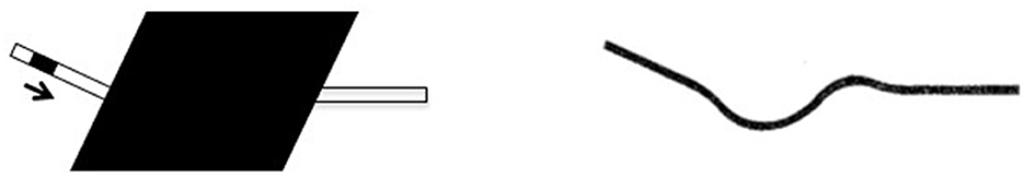
Figure 2. The (left) picture illustrates the coincidentally occluding tunnel studied by Burke (1952). A small rectangle (5 × 15 mm) moved from left to right (as indicated by the arrow) along entry and exit slits at the speed of 300 mm/s: the tunnel was 75 mm long horizontally. Four entry-exit intervals were studied (75, 180, 250, and 600 ms). Observers were seated at 1.5 m from the apparatus (Michotte's disks). The (right) picture illustrates one of the continuous trajectories reported by observers at short entry-exit intervals; namely, a smooth non-monotonic curve consistent will the misperception of the horizontal exit slit as “too high.” Redrawn from the original Figure 1B by Burke (1952, p. 123).

Gerbino (1978) used a pattern similar to Figure 1B and a sliding occluding triangle to find in which position the point where the near edge meets the occluding edge appeared aligned with the extrapolation of the far edge; this position, where the perceived misalignment was nulled, provided an estimate of the expansion of the near edge (about 7% of the near edge length). As regards the shape of the amodally completed angle, at first glance Gerbino's observers described a rather indeterminate continuation of angles of the hexagon behind occluding triangles; despite its indeterminateness, the feeling of presence of a vaguely defined protuberance behind each triangle in Figure 1B is enough to account for the loss of regularity of the coincidentally occluded hexagon. Gerbino (1978) also reported specific completions obtained after prolonged observation (Figure 1F), equivalent to the smooth but non-monotonic trajectory illustrated by Burke (1952) in his Figure 1B, depicting a tunnel coincidentally aligned with the vertex of the angle formed by entry and exit trajectories (Figure 2).

As regards the second effect, the hypothesis that the T-stem misorientation is the actual cause of the perceived misalignment between the far edge and the corresponding angle's vertex was already considered by Gerbino (1978), by analogy with some explanations of the Poggendorff illusion (Weintraub and Krantz, 1971; Robinson, 1972). Gerbino (2017, 2020) discussed a possible origin of such misorientation, based on the notion of visual approximation (see next subsection). However, no attempt to measure the perceived orientation of the sides of the hexagon in the Gerbino illusion has been made before the present study.

As regards the third effect—the impression of rotation—observers who distribute their attention globally perceive the patterns in Figures 1C, D as conveying a rotary sensation, though reports of its direction, CW or CCW, are not always explicit. The global rotation induced by the Gerbino illusion display has been studied by Fantoni et al. (2007), who presented observers with a dynamic sequence in which either Figure 1C or Figure 1D was shown, followed by a 200 ms blank interval and then by Figure 1A. When the first frame displayed Figure 1C (CCW occlusion), the unoccluded hexagon in the second frame underwent a CW rotation; when the first frame displayed Figure 1D (CW occlusion), the unoccluded hexagon in the second frame underwent a CCW rotation. Considering that occluded and unoccluded hexagons shared the same objective orientation, this means that the coincidentally occluded hexagon appeared globally rotated in the direction homologous to the direction of its occlusion (i.e., the CCW occlusion in Figure 1C induced a CCW tilt, whereas the CW occlusion in Figure 1D induced a CW tilt).⁶ This global rotation effect is consistent with the visual approximation framework, if one presupposes that presentation of the first frame instantiates an internal model of the visual scene in which the orientation of the sides of the hexagon is misperceived to generate a smooth monotonic amodally completed contour.

However, the global rotation studied by Fantoni et al. (2007) could also be interpreted as a configural effect induced by the asymmetric off-axis placement of triangles. Pinna (2012, Figure 3) discussed the Gerbino illusion and mentioned a spiral-like deformation apparently associated with the global rotation, without specifying its direction. Pinna (2012) also argued that AC cannot be considered the cause of the spiral-like deformation observed in the Gerbino illusion display, given that similar deformations are also obtained in the absence of AC. As remarked by Gerbino (2020), Pinna's demonstration that other figural manipulations (different from the superposition of coincidentally occluding triangles) can induce a spiral-like deformation does not disprove that AC is a condition (sufficient, yet not necessary) for the occurrence of such effect. In particular, Pinna's Figure 9I mimics the protrusions that would be generated by smooth non-monotonic interpolations of far and near edges. This further suggests that AC might be considered the remote cause of the spiral-like deformation: in other terms, occlusion might set the conditions for amodal protrusions that—independently of their degree of determinateness—produce functional effects comparable to those produced by the actual addition of smooth off-axis protrusions to the contour of a regular unoccluded polygon.

1.3. Two completion frameworks

As anticipated in the preceding subsection, two alternative frameworks have been proposed to explain the AC of coincidentally occluded angles: visual interpolation and visual approximation.

1.3.1. Visual interpolation framework

Within the visual interpolation framework AC is mediated by the extrapolation-interpolation of veridically represented T-stems (Gerbino, 1978, 2017, 2020). The perceived distortion of coincidentally occluded angles would depend on the irresistible tendency to extrapolate contours behind occluders (Figure 1E), possibly combined—at least for some observers—with the interpolation of a smooth but necessarily non-monotonic amodal contour. Such non-monotonic interpolation of a coincidentally occluded angle would be characterized by the point of inflection shown in Figure 1F. As mentioned before, visual interpolation cannot account for the observation that the near edge appears to be intersected by the extrapolated far edge in its visible part (consistently with the above-mentioned paradoxical expansion of modal parts).

1.3.2. Visual approximation framework

Within the visual approximation framework (Fantoni et al., 2007, 2008a; Gerbino, 2017, 2020) the visual system copes with coincidental occlusion by generating an amodally completed rounded polygon whose smooth monotonic contour minimizes the deviation from input fragments. The generation of a monotonic amodal contour should be achieved at the expense of veridicality, by misrepresenting the orientation of T-stems in the homologous direction. This inaccurate encoding of T-stem orientations would support the recovery of a legal interpolation triangle behind each occluder.

Take Figure 1C, where angles are occluded in the CCW direction. According to the approximation-based model in Gerbino (2020, Figure 7C), the AC of coincidentally occluded angles includes two stages: in an early stage smoothness and monotonicity constraints lead to the generation of a rounded hexagon whose visible sides are misrepresented in the homologous CCW direction (Figure 1G); in a later stage, instead, the conflict between input evidence and the misoriented hexagon constrained by smoothness and monotonicity is experienced as a perceptual distortion of the sides of the hexagon in the opposite CW direction (Figure 1H).

The visual approximation framework is supported by evidence that AC processes elicited by limiting cases of occlusion instantiate non-veridical modal parts that minimally deviate from input fragments. More generally, the visual approximation framework accounts for the following phenomena in pictorial and 3D domains:

1) Partially occluded Vernier bars are perceptually distorted toward collinearity (Mussap and Levi, 1995; Gerbino et al., 2006);

2) In weak stimulus support conditions (Rock, 1983) a square with partially occluded angles is perceptually rounded; in particular, as the retinal size of contour gaps gets smaller, the perceptual rounding of the amodally completed shape progressively increases, consistently with the hypothesized dominance of the minimal path tendency over the good continuation tendency (Fantoni and Gerbino, 2003; Gerbino, 2017);

3) A pair of 3D partially occluded laminas is perceptually distorted toward coplanarity, to compensate for their offset (Liu et al., 1999; Hou et al., 2006), relative tilt (Fantoni et al., 2008a) or relative slant (Fantoni et al., 2008b), showing that AC supports the formation of a smooth surface that minimizes depth offset and torsion, and optimizes the 90° relatability constraint.

1.3.3. Difference between interpolation- and approximation-based solutions

Ordinarily, AC has been modeled within the visual interpolation framework (Ullman, 1976; Horn, 1983; Kellman and Shipley, 1991; Fantoni and Gerbino, 2003), probably because in most cases interpolation- and approximation-based predictions converge. However, when the geometry of T-stems is incompatible with smoothness and monotonicity constraints (Figures 1C, D), interpolation- and approximation-based solutions do differ.

According to visual interpolation (Gerbino, 1978), the perceived hexagon of the Gerbino illusion would be characterized by the concatenation of modal parts that veridically represent the orientation of input fragments while amodally continuing behind occluding triangles, with the global impression of rotation attributed to the local protrusions due to the smooth non-monotonic joining of consecutive T-stems.

According to visual approximation, instead, the generation of amodal parts could affect also modal parts (Fantoni and Gerbino, 2003; Fantoni et al., 2008a; Gerbino, 2017, 2020). In particular, the visual approximation of a coincidentally occluded hexagon (Figures 1C, D) would imply the perceived misorientation of T-stems, in compliance with smoothness and monotonicity constraints.

2. Materials and methods

Our study aimed at measuring the possible misorientation of two consecutive T-stems of the Gerbino illusion display, predicted by visual approximation but not visual interpolation, controlling for possible distortions unrelated to AC. Separate groups of participants were shown one of the three displays in Figure 3.

a) The experimental AC display (Figure 3A) was expected to elicit the hypothesized AC-dependent distortion.

b) The No-completion display (Figure 3B) was a control for a possible perceived distortion independent of AC, due to the off-axis placement of triangles; i.e., to a perturbation of the hexagon's symmetry that might induce a rotary sensation in the homologous direction (CCW, for patterns in Figures 3A, B).

c) The Mosaic display (Figure 3C) was a control for a possible spiral-like effect specifically induced by the literal shape of the unoccluded region of the hexagon in Figure 3A.

FIGURE 3

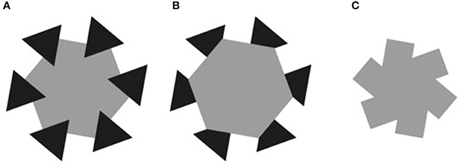
Figure 3. The three displays utilized in our study: (A) AC display; (B) No-completion display; (C) Mosaic display.

To measure the perceived orientation of the sides of the hexagon we envisioned a novel technique inspired by the sequential probing procedure that Fulvio et al. (2008) adopted to estimate the shape of the amodal contour joining two oblique T-stems.⁷ Their participants were free to toggle back and forth between position and orientation adjustments of a short line revealed by a slit in the occluding rectangle, until the combination of settings optimized a smooth amodal contour joining the two T-stems. Fulvio et al. (2008) studied three T-stem offset conditions: null; small (consistent with co-circularity); large (inconsistent with co-circularity). Accuracy and precision of probe position and orientation decreased as the offset increased, approaching a coincidental occlusion condition. However, the effect found by Fulvio et al. (2008) might at least partially depend on acute angle expansion, irrespective of AC, given that their T-junctions were oblique, like in the classic Poggendorff display.

Our study overcomes three major limitations of the study by Fulvio et al. (2008). The first concerns the control for distortions due to T-junction geometry, independent of AC; contrary to displays used by Fulvio et al. (2008), our experimental display (Figure 3A) features orthogonal T-junctions and allows us to exclude the tendency to acute angle expansion from the range of possible explanations of the hypothesized misorientation effect. The second regards the consistency of the two adjustments produced by participants, which Fulvio et al. (2008) calculated on the basis of deviations from an interpolated path joining two undistorted fragments. Such a measure assumes the validity of the visual interpolation framework and might be inappropriate when occlusion is highly asymmetric, like in the Gerbino illusion display, and the perceived distortion of modal contours fits the visual approximation framework. The third regards the measurement technique: participants in the study by Fulvio et al. (2008) toggled back and forth between position and orientation adjustments, with the risk that such adjustments reflect multiple interpolated paths instead of a single one, while in the present study we used a simple two-phase adjustment technique.

Consider the AC display (Figure 3A). To estimate the perceived orientation of each side of our target angle (the top-left angle of the coincidentally occluded hexagon), we asked participants to perform two sequences of extrapolation and tilt adjustments, one for each direction of the same side. The extrapolation adjustment consisted in moving a distal dot along a circular path, to make it collinear with the selected side of the target angle. The circular path of the dot probe (Figure 4: blue circle for the left side; orange circle for the right side) was centered on the unoccluded side midpoint, thereby keeping constant the distance between the probe and endpoints of the unoccluded side in AC and Mosaic conditions.⁸

FIGURE 4

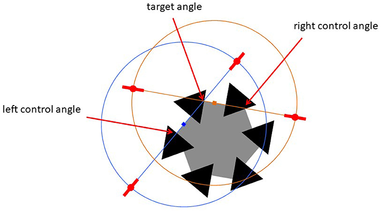
Figure 4. The circular paths of probes utilized to estimate the orientation of the two sides of the target (top-left) angle in the AC display [blue for the (left side), orange for the (right side)]. Each circular path was centered on the midpoint of the unoccluded portion of the relevant side. The circular probe paths were the same also for No-completion and Mosaic displays.

As shown in Figure 5, the tilt adjustment was always performed after the extrapolation adjustment and consisted in adjusting the tilt of a distal segment centered on the adjusted dot, to match the perceived tilt of the relevant T-stem.

FIGURE 5

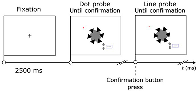
Figure 5. Temporal sequence of a two-phase trial (AC condition, right side, near edge). After a fixed 2,500 ms intertrial interval the participant moved the red dot along the circular path shown in Figure 3 by pressing arrows, to make it collinear with the extrapolation of the right side of the target angle. After pressing of the confirmation button, the probe became a short segment, whose tilt could be adjusted (again, by pressing arrows) to match the tilt of the same side of the hexagon.

In No-completion and Mosaic control conditions participants were required to perform the same task on the corresponding sides of displays in Figures 3B, C. Importantly, our probes were outside the occlusion region and rather far from it, to reduce the risk of interference with AC processes.

Finally, under the assumption that coincidentally occluded angles set the conditions for visual approximation, we analyzed the individual pattern of two-phase adjustments in an unsupervised way, using cluster analysis; i.e., without referring them to either the target or control angles (i.e., the factor Angle of our experimental design) or the respective far or near edges (i.e., the factor Edge of our experimental design). The extrapolation-tilt technique provided us with four orientation measures for each side of the target angle (two for each endpoint of its left and right sides), which were expressed as angular deviations from the actual edge orientation. Depending on the output of the cluster analysis the number of groupings of such deviations could be smaller than four (the number of Angle × Edge combinations).

2.1. Expectations

To interpret expected errors in extrapolation and tilt adjustments, we considered a fundamental implication of an approximated AC solution, which we suggest to call the approximation constraint. Within the visual approximation framework, a coincidentally occluded angle can be amodally completed along a smooth monotonic path only if the orientation of T-stems is misrepresented, in a direction compatible with the construction of a legal interpolation triangle. This misrepresentation might involve both the far and the near edge of a coincidentally occluded angle or only the far edge.⁹

For the sake of generality we expected that in our AC condition—at least more than in the two control conditions—extrapolation and tilt errors relative to the far edge were in the CCW direction; i.e., laying in the first quadrant of the extrapolation-tilt error space and scattered along its positive diagonal (Figure 6). Errors were expected to occur in the homologous CCW direction if they reflect the first stage of the hypothetical approximated AC, corresponding to an internal model allowing for the construction of a legal interpolation triangle.¹⁰

FIGURE 6

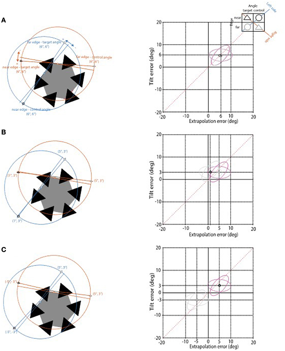
Figure 6. Hypothetical patterns of extrapolation and tilt errors for Angle × Edge combinations illustrated in the top-right inset. Errors in the homologous CCW direction are positive. In each panel the error pattern for the AC display shown on the left is plotted in the extrapolation-tilt error space on the right. In Figure 7 this space will be used also to represent the cluster analysis results. (A) Illustrates a globally consistent solution, with all extrapolation and tilt errors equal, corresponding to the rigid rotation of the hexagon illustrated in Figure 1G. (B) Illustrates a case, consistent with the collinearity assumption, in which each extrapolation error differs from the paired tilt error, leading to different extrapolation errors for the two edges of the same side, but with the same error pattern for the two sides. (C) Illustrates a violation of the collinearity assumption, with error pairs in the CCW direction for far edges and in the CW direction for near edges.

Consistently with the approximation constraint, at least three possible AC solutions can be distinguished.

2.1.1. Globally consistent solution

A uniform misrepresentation of both CCW and CW sides (relative to the target angle considered in our experiment) would lead to the same error in each Angle × Edge × Probe adjustment (left panel of Figure 6A). In the extrapolation-tilt space (right panel of Figure 6A) the four points representing the paired errors for each Angle × Edge combination would collapse into the same location along the space diagonal; specifically, in the first quadrant of the extrapolation-tilt space, given that all errors are in the CCW direction. The globally consistent solution would correspond to a reduced number of error groupings, from four (one for each Angle × Edge combination) to one (single Cluster condition). The single-cluster condition would group all errors and collapse them into a single maximum likelihood estimate (the cluster centroid) with equal positive coordinates in the extrapolation-tilt space.

2.1.2. Collinear solution

A more generic and likely solution might involve different amounts of extrapolation and tilt errors for the same edge, but with probes relative to opposite edges of the same side adjusted to be collinear (left panel of Figure 6B). According to the collinearity assumption (see Appendix 1 of the Supplementary material for details), the error pair (ε, τ) for one edge and the error pair (ε', τ') for the opposite edge are linked by the following equations:

$\begin{array}{ll}{\epsilon }^{\prime }=2\tau -\epsilon ;& (1)\end{array}$

$\begin{array}{ll}{\tau }^{\prime }=\tau .& (2)\end{array}$

This solution would be characterized by the generation of a legal interpolation region similar to the one obtained in the globally consistent solution, combined with the overrepresentation of the partially occluded hexagon size (a potentially interesting aspect not considered in our experimental design). In the extrapolation-tilt space (right panel of Figure 6B), the collinear solution would be represented by the superposition of the two points relative to homologous edges (either far or near).

The collinear solution would correspond to a reduced number of error groupings, from four (one for each Angle × Edge combination) to two (two Cluster conditions). The two-cluster conditions would group errors into two maximum likelihood estimates according to Edge type, with equal positive tilt, but different positive extrapolation coordinates in the extrapolation-tilt space (far edge cluster larger than near edge cluster).

2.1.3. Non-collinear solution

A further generic solution might violate the collinearity assumption (with error pairs not linked by Equations 1 and 2), but be consistent with the approximation constraint, with errors relative to far edges in the CCW direction, irrespective of Angle type. The left panel of Figure 6C depicts a specific example in which probe adjustments are biased toward the hexagon's center, with errors relative to far edges in the homologous CCW direction and errors relative to near edges in the non-homologous CW direction.

In the extrapolation-tilt space (right panel of Figure 6C) such non-collinear solution would correspond to the grouping of points according to Edge type. Like the collinear solution, also the non-collinear solution would correspond to a reduced number of error groupings, from four (one for each Angle × Edge combination) to two (two Cluster conditions). Here, the two-cluster conditions would group errors into two maximum likelihood estimates according to Edge type, with groupings for far and near edges laying in the first (positive-positive) and third (negative-negative) quadrants of the extrapolation-tilt space, respectively.

2.2. Cluster analysis

Consider the 2-fold advantage of the above described formalization of possible AC solutions and error patterns. First, it allowed us to evaluate the possible deviation of the obtained error pattern from AC solutions that preserve the shape of the hexagon (the first two, globally consistent and collinear) in favor of an AC solution, dependent on Edge type, that would imply a paradoxical disruption of the shape of the hexagon. Second, it provided us with the possibility of grouping every pair of extrapolation and tilt errors associated with any Display (3) × Angle (2) × Edge (2) condition into one of two unsupervised clusters, on the function of either Angle type, according to a shape-preserving AC solution, or Edge type, according to a shape-disrupting AC solution.

To evaluate our expectations we first analyzed extrapolation and tilt errors separately (Appendix 2 in the Supplementary material). Then, we applied an unsupervised cluster analysis to individual adjustments, controlling if extrapolation and tilt errors grouped into two clusters, treatable as a 2-level factor Cluster. This further factor should account for how the covariation between extrapolation and tilt errors is modulated by the Angle × Edge combination across different conditions. The Cluster factor might group errors relative to different Angle and/or Edge types along the diagonal of the extrapolation-tilt space, with the medians of cluster centroids representing the maximum likelihood estimates of adjustment errors. As a consequence, the relevant part of a statistic accounting for the variability of tilt errors as a function of Display, Angle, Edge, and Extrapolation Error should be reducible to a simpler one including only Display, Extrapolation Error and Cluster as factors. In particular, we expect to obtain a significant 3-way interaction, with the Extrapolation Error × Cluster interaction being significant in AC but not control conditions.

Such expectations can also be reframed expressing each individual adjustment in terms of its likelihood to be categorized as belonging to Cluster 1. We used this further dependent measure as diagnostic of the type of process driving the perceived solution as well as the type of distortion. The distribution of the likelihood of adjustment errors to belong to Cluster 1 involved in a distorted representation of input fragments will differ from the one involved in their literal representation, expected in the two control conditions, as well as in the AC condition under visual interpolation.

2.3. Participants

Sixty participants were recruited using an online form [F = 46; average age = 21.9 ± 2.9 SD; age range = (19–33)]. They were psychology students, naïve to the specific hypothesis of the study, with normal/corrected-to-normal visual acuity. The experiment was conducted online, because of restrictions dictated by the COVID-19 pandemics. Participants were tested individually to keep them motivated throughout the experiment and to minimize uncontrolled effects of the online procedure on their overall performance (Germine et al., 2012). Each participant was contacted by the experimenter (AD) via Microsoft Teams™ and accessed the computer hosting the experiment program via a TeamWork™ link. The online recruiting form provided the participant with a list of requirements to take part in the experiment, including:

1) A university account to access Microsoft Teams™ and a personal computer compatible with TeamWork™;

2) Laptop or desktop computer with minimum screen size of 14 inches and 1920 × 1080 screen resolution (mobile devices not permitted);

3) Instructions to use Teams™ to interact with the experimenter on the experimental day (to communicate the general aim of the experiment, data-handling procedures, and task instructions);

4) The request to keep their webcam open throughout the experiment, allowing the experimenter to control lighting and acoustic conditions.

We conducted a sensitivity analysis with G-Power 3.1 (Faul et al., 2007) on our sample size with α err. Prob. = 0.05, Power (1 – β err. Prob.) = 0.90 to establish the Minimal Detectable Effects for our experimental design. These resulted to be in the small-to-medium range with a critical F = 1.71 and a ${\eta }_{\text{p}}^2$ = 0.05.

2.4. Stimuli

Stimuli were centered on the screen of a MSI GT73VR computer hosted in our laboratory and were controlled by a custom-made script in VBA (Visual Basic for Applications) within Microsoft PowerPoint 2018 under Windows 10. To control the execution of the program the experimenter remotely shared the laboratory screen via a TeamWork™ link. To equate the retinal size of stimuli, irrespective of individual screen size, at the beginning of the experiment the participant was asked to hold her thumb at arm length and to set her distance from the screen so that the thumb matched a red circle at the center of the screen of about 2 cm of diameter (on the laboratory screen). In the following, stimulus measures are contingent on the assumption that the red circle subtended 2° of visual angle.

The experimental AC display consisted of a gray (RGB: 127, 127, 127) hexagon with six equilateral black triangles coincidentally occluding its angles (Figure 3A). The side of occluding triangles subtended 2.5° of visual angle. The right side of target angle was tilted 10° in the CW direction. Every unoccluded portion of the sides of the hexagon was characterized by two orthogonal T-junctions. In the No-completion display the hexagon was fully specified and occluded part of the black triangles (Figure 3B). The Mosaic condition was obtained by turning white the occluding triangles of the experimental display, making them indistinguishable from the background (Figure 3C).

To measure the perceived orientation of sides of the target (top-left) coincidentally occluded angle in the AC display and of the corresponding sides in control displays we used two sequentially presented probes, a dot and a line. The dot probe subtended about 0.25° of visual angle and could be moved along an invisible circular path of radius 5°, centered on the midpoint of the unoccluded portion of the relevant side of the AC display, until it appear to lie on its extrapolation. The line probe was 0.25° thick and 1° long and could be rotated around the confirmed position of the dot probe, to match the perceived tilt of the measured side. The initial position of the dot probe along the circular path and the tilt of the line probe were randomly and independently selected within an error range of [−20°, +20°], chosen to be large enough to ensure that extreme adjustments were clearly perceived to be wrong, for either extrapolation or tilt.

Participants adjusted the position of the dot probe along the circular path and the tilt of the line probe by means of two gray arrow buttons (RGB: 127, 127, 127; 2.17° × 2.37°; Figure 5). For both adjustments (extrapolation and tilt) an arrow button press caused a change of orientation of about 1°, in CCW-CW directions for top-bottom arrows, respectively. A press of the confirmation button (2° × 4°; Figure 5) caused the ending of the adjustment phase and the storage of the confirmed value.

2.5. Design and procedure

The experiment included 24 conditions resulting from the mixed combination of Display (AC, No-completion, Mosaic) × Angle (target, control) × Edge (far, near) × Probe (dot, line), with the Display factor manipulated between subjects. Participants were randomly assigned to one of the three Display conditions, in a full balanced fashion. The experiment was conducted individually, using Microsoft Teams™ for communication and participant monitoring throughout the procedure. Specifically, our online process comprised three successive phases described below.

2.5.1. Screen setting

At the start of the videocall, the experimenter assessed the participant's device type, screen size, and resolution by requesting them to share their screen and access the screen settings. If needed, the experimenter guided the participant to adjust the screen resolution to the required settings (1920 × 1080 pt).

2.5.2. Room setting

The participant was initially asked to use their webcam to show the desk and the room where they would be during the experiment. The experimenter carefully ensured that the participant was alone in the room and that there were no acoustic or visual distractions present. Subsequently, the participant was instructed to turn off room lights and given access to the experiment by providing the TeamWork™ link.

2.5.3. Calibration

To maintain constant control over the retinal size of the stimuli and variations in visual angle during the experiment, we diligently calibrated the participants' distance and position relative to the screen. For the visual angle calibration, participants were shown a red circle at the center of the screen and were instructed to keep their torso and head upright and frontal. Under the experimenter's supervision, participants adjusted the vertical and horizontal position of their head relative to the screen center. Those who could not adjust their position relative to the screen were excluded. Regarding the calibration of the retinal size of the stimuli, participants were instructed to follow the procedure based on the “thumb” rule outlined in the “Stimuli” subsection.

2.5.4. Experiment

The experiment was introduced by on-screen instructions and a brief video tutorial that informed participants on how to adjust the dot and line probes using the two on-screen arrow buttons. After reading instructions, the participant performed four practice trials in which dot and line probes were adjusted to match the orientation of one side of an equilateral triangle (side = 3°) centered on the screen. Each experimental trial included the following phases, depicted in Figure 5:

1) A black fixation cross appeared on the center of the screen for 1.5 s;

2) The cross was substituted by the display, which appeared together with the dot probe, whose position was randomly selected in the ±20° range relative to the extrapolation of the to-be-measured edge;

3) After the confirmation button press the line probe substituted the dot probe in the confirmed position, with a tilt randomly selected in the ±20° range relative to the tilt of the to-be-measured edge;

4) After the confirmation button press the next trial began.

The individual experimental session included 32 trials corresponding to the combination of Angle (2) × Edge (2) × Probe (2) × Repetition (4). The order of the four Angle × Edge blocks of eight trials was randomly selected and balanced across subjects. Completing the experimental session took about 10 min (mean = 10.2 min, SD = 5.2 min). The experimenter provided the participant with careful guidance throughout the entire experiment. Furthermore, the participant position and distance from the screen were continuously monitored using the webcam.

2.6. Data analysis

To test our expectations on possible visual approximation effects in AC but not control conditions, we extracted two indices of performance in our sequential adjustment task: (1) the individual values of extrapolation and tilt errors (separately analyzed in Appendix 2 of the Supplementary material); (2) the individual likelihood of errors to belong to one of two partitioning groups determined through the unsupervised cluster analysis.

For both extrapolation and tilt, errors in the CCW direction (with respect to the objective orientation of the relevant edge) were labeled positive and those in the CW direction negative.

Out of 640 adjustments within each Display condition, resulting from the combination of 20 participants × Angle (2) × Edge (2) × Probe (2) × Repetition (4), we found the following number of missing values: 14 in the AC condition, 0 in the No-completion condition, 11 in the Mosaic condition. Then, we restricted our analysis to valid trials by performing a separate outlier analysis on the remaining errors and fitting data within each Display condition with a linear mixed effect model with maximal complexity, MAXlmer, including all interactions and main effects for the Angle × Edge × Probe design, with the maximal random effects structure justified by it (Barr et al., 2013). We considered as valid trials those in which both extrapolation and tilt errors fell inside ±2.5 SD from the predicted value of the MAXlmer. The final numbers of valid trials were: 570 in the AC condition, 590 in the No-completion condition, and 588 in the Mosaic condition.

As regards our second index of adjustment performance, we followed the procedure anticipated in Subsection 1.5. In particular we used the k-means() function of the {stats} package to perform an unsupervised cluster analysis on the tilt errors expressed as a function of their corresponding extrapolation errors, for each Display condition. We used the NbClust() function of the {NbClust} package to determine the optimal number of clusters describing each individual set of joined adjustment errors. Specifically, this function determines the partitioning of groups of errors based on the identification of validation indices optimally accounting for the best clustering scheme obtained with the k-means clustering method, by varying the number of clusters from 2 to 15 [the default value in NbClust(); Charrad et al., 2014]. As expected, the majority of validation indices (out of a total number of 23) were accounted for by two clusters. The two-cluster solution was therefore selected on the basis of the best values obtained on seven out of 23 indices in the AC condition, six out of 23 indices in the No-completion condition, and four out of 23 indices in the Mosaic condition.

In order to test the different perceptual solutions driving adjustments across displays we performed two major analyses, one for each index of performance in our two-phase adjustment task: (1) a MAXlmer analysis on the distribution of valid tilt errors with Cluster, Display, Angle and Edge as fixed factors, and valid extrapolation error as a covariate, testing how much the Cluster factor accounted for the combination of Display × Angle × Edge; (2) a MAXglmer analysis on the likelihood distribution of joined errors to belong to Cluster 1, with Display, Angle and Edge as fixed factors.

To evaluate two specific implications of an approximated AC solution, described in Subsection 1.4 as the approximation constraint and the global consistency constraint, we performed the following two tests.

Test 1 (approximation constraint). We estimated the deviation of average extrapolation and/or tilt errors from the null value at the point of maximum likelihood as expressed by cluster centroids. To this aim, adjustment errors belonging to each cluster were fitted by a lmer model of Extrapolation × Tilt and the significance of lmer estimates from null values was computed entering the corresponding cluster centroid coordinates.

Test 2 (global consistency constraint). We performed an analysis predicting observed adjustment errors in the four Angle × Edge conditions with cluster centroids extracted according to the global consistency constraint. To this aim, we used cluster centroids as maximum likelihood estimates of the distribution of adjustment errors belonging to them. We quantified the amount of deviation of each pattern of observed errors from a globally consistent AC solution using a Welch's one-sample t-test.

As statistical inferential measures we provided: (1) type III-like two-tailed p-values for significance estimates of MAXlmer/MAXglmer fixed effects and parameters adjusting for the F-tests the denominator degrees-of-freedom with the Satterthwaite approximation; (2) estimates of effect size based on the concordance correlation coefficient r_c and partial eta squared ${\eta }_{\text{p}}^2$ (for interactions and main effects of F-tests); (3) AIC, BIC, loglikelihood, and overall residual deviance as estimates of the relative quality of models.

3. Results

Figure 7 depicts how the two-cluster solutions (with orange and gray ellipses encoding Clusters 1 and 2, respectively) accounted for individual extrapolation × tilt errors in AC (panel a), No-completion (panel b) and Mosaic (panel c) displays. The four Angle × Edge combinations are encoded by shapes and lightnesses specified in the top-right legend (the same as in Figure 6).

FIGURE 7

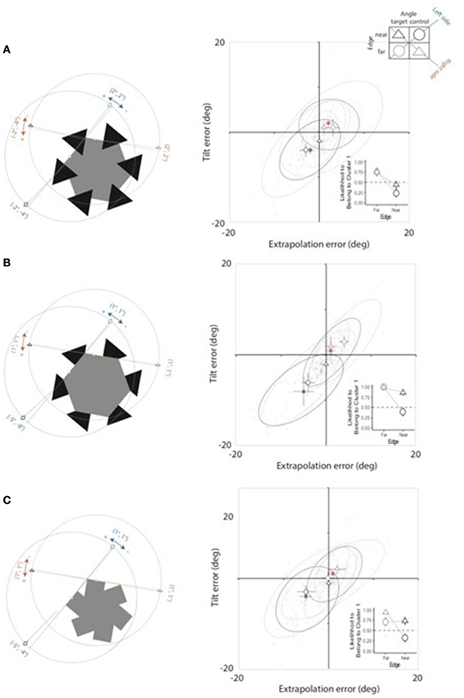
Figure 7. Obtained adjustment errors in each Display condition [(A–C) for AC, No-completion, and Mosaic displays, respectively]. Sketches on the left depict the Angle × Edge pattern of adjusted probes and their linear extensions. Represented values have been chosen to match the median of the cluster to which each error resulted to be more likely to belong. The corresponding plots on the right depict the mapping of such values in the error space introduced in Figure 6, together with the distribution of individual (outline symbols) and average (filled symbols) errors, with each inset showing the average likelihood of errors to belong to Cluster 1 in each Angle × Edge condition (see text for details).

For the ease of comprehension, the most likely probe solution is shown in the sketches on the left. Visualized adjustment errors correspond to the median extrapolation and tilt error of the cluster to which it is more likely to belong.

The pattern of errors categorized according to the two clusters is markedly different across Display conditions, with errors in the AC condition (Figure 7A) being different from those in the two control conditions (Figures 7B, C). Errors relative to different Edge types grouped into different clusters, with Cluster 1 grouping errors referred to the far edge in the first quadrant of the extrapolation-tilt space (consistently with the approximation constraint) and Cluster 2 grouping errors referred to the near edge in the third quadrant. In particular, Figure 7A shows that in the AC condition the perceptual solution extracted through the cluster analysis well accounts for the individual pattern of errors in the four Angle × Edge conditions, according to a non-collinear solution; i.e., with the amodal presence of a shrinked target angle rotated in the CCW direction.

As depicted in the left sketch of Figure 7A, the obtained estimates of the orientation of the two far edges (continuous lines) deviate from the objective orientation of the reference sides (dotted lines) in the CCW direction, by amounts corresponding to the coordinates of the Cluster 1 centroid (2° and 2°, for extrapolation and tilt errors, respectively). On the contrary, the obtained estimates of the orientation of the two near edges deviate from the objective orientation of the reference sides in the CW direction, by amounts corresponding to the coordinates of the Cluster 2 centroid (−2° and −4°, for extrapolation and tilt errors, respectively). Importantly, the extrapolations of near and far edges of the target angle form an angle which is 4° smaller than the one defined by input fragments and slightly rotated of about 2° in the CCW direction, thus allowing for the formation of a legal interpolation region.

This solution is consistent with the distribution of likelihood shown in Figure 7A inset, with the likelihood of errors to belong to each cluster being well-balanced over Edge type, irrespective of Angle type, with far edge adjustments being accounted for by Cluster 1 (collecting values above chance level) and near edge adjustments being accounted for by Cluster 2 (collecting values below chance level).

Adjustments in the AC condition differed from those in control conditions, that instead closely matched the input geometry. In both control conditions the adjustments relative to the target angle are equal to those for the far edge of the control angle, corresponding to the slight CCW rotation described by the (1°, 1°) coordinates of the Cluster 1 centroid. The difference between AC and control conditions is further supported by the distribution of likelihood of errors to belong to Cluster 1 (insets in Figures 7A–C). In AC condition the pattern of the likelihood of errors to belong to Cluster 1 is markedly different from the funnel-like pattern observed in both control conditions. This pattern is diagnostic of a veridical representation of input fragments.

In the two subsections below, we show that these observations are statistically supported by converging evidence from two different synthetic measures of adjustment performance.

3.1. Individual adjustment errors

First, we considered the individual pattern of tilt errors and contrasted the goodness of fit of two MAXlmer models: one including Display, Angle, Edge, and Extrapolation Error as fixed effects (MAXlmer1: r_c = 0.91) vs. another including Cluster as an additional factor (MAXlmer2: r_c = 0.93). Importantly, MAXlmer2 accounted for the great majority of main effects and interactions revealed by MAXlmer1, nulling five out of the six significant effects revealed by MAXlmer1: the main effects of Edge [F_(1,60.62) = 18.61, p < 0.001, ${\eta }_{\text{p}}^2$ = 0.23] and Extrapolation Error [F_(1,475.27) = 347.23, p < 0.001, ${\eta }_{\text{p}}^2$ = 0.42]; the 2-way Display × Extrapolation Error interaction [F_(2,337.32) = 13.17, p < 0.001, ${\eta }_{\text{p}}^2$ = 0.07], and three 3-way interactions [Display × Angle × Edge: F_(1,440.80) = 4.45, p = 0.035, ${\eta }_{\text{p}}^2$ = 0.09; Display × Edge × Extrapolation Error: F_(2,318.59) = 6.33, p = 0.002, ${\eta }_{\text{p}}^2$ = 0.04; Display × Angle × Extrapolation Error: F_(2,361.18) = 11.78, p < 0.001, ${\eta }_{\text{p}}^2$ = 0.06].

This result revealed that the best fitting model (MAXlmer3) should include only the Display × Extrapolation Error × Cluster interaction as a fixed effect (r_c = 0.88). MAXlmer3, though including much less free parameters than MAXlmer1 (34 vs. 103), accounted for a similar proportion of variance (R² = 0.83 for MAXlmer1; R² = 0.80 for MAXlmer3) and optimized the goodness of fit according to all major fit indices: AIC (4,394.2 vs. 4,597.9), BIC (4,990.8 vs. 5,089.5), loglikelihood (−2,072.1 vs. −2,195.9), overall residual model deviance (4,144.2 vs. 4,391.9).

In particular, all effects revealed by MAXlmer3 agreed with our expectation that the Cluster factor would account for the way the Angle × Edge combination modulated the covariation between extrapolation and tilt errors across Display types, consistently with a visual approximation effect in the AC condition but not in control conditions. The MAXlmer3 model included the only main effect of Extrapolation Error predicted by MAXlmer1, with tilt errors increasing proportionally with extrapolation errors at a rate of β = 0.59 ± 0.02 [t_(706.58) = 20.86, p < 0.001].

Furthermore, MAXlmer3 revealed the following set of effects: a main effect of Cluster [F_(1,59.20) = 108.08, p < 0.001, ${\eta }_{\text{p}}^2$ = 0.44], with a positive estimated tilt error for Cluster 1 (1.90 ± 0.18) vs. a negative estimated tilt error for Cluster 2 (−5.88 ± 0.29); a main effect of Display [F_(2,53.71) = 11.42, p < 0.001, ${\eta }_{\text{p}}^2$ = 0.22], due to significant difference between the tilt error in the Mosaic condition relative to the other two conditions (AC: −0.65 ± 0.31; No-completion: −0.64 ± 0.43; Mosaic: −0.50 ± 0.27); a 3-way Display × Extrapolation Error × Cluster interaction [F_(2,137.08) = 8.45, p < 0.001, ${\eta }_{\text{p}}^2$ = 0.08], consistent with a different pattern of adjustments across the three Display types.

The positive relationship between tilt and extrapolation errors was significant for responses of Cluster 2 [β = 0.56 ± 0.09, t_(272.39) = 6.09, p < 0.001] but not for responses of Cluster 1 [β = 0.10 ± 0.08, t_(278.57) = 1.21, p = 0.227] in the AC condition. Vice versa, it was significant for responses of both clusters in the No-completion control condition [Cluster 1: β = 1.10 ± 0.05, t_(293.00) = 19.71, p < 0.001; Cluster 2: β = 0.95 ± 0.09, t_(293.00) = 10.00, p < 0.001], as well as in the Mosaic condition [Cluster 1: β = 0.39 ± 0.04, t_(234.83) = 8.10, p < 0.001; Cluster 2: β = 0.24 ± 0.07, t_(83.82) = 3.32, p = 0.001].

3.2. Likelihood of belonging to Cluster 1

To further support the different types of perceptual solutions driving adjustments across conditions we performed a MAXglmer analysis (r_c = 0.77) on the likelihood of adjustments to belong to Cluster 1, including Display, Angle, and Edge as factors. This analysis revealed: (1) a main effect of Edge [F_(2,851) = 47.05, p < 0.001, ${\eta }_{\text{p}}^2$ = 0.68], with the likelihood of errors relative to the far edge (0.93 ± 0.20) to belong to Cluster 1 being larger than the likelihood of errors relative to the near edge (0.48 ± 0.10); (2) a main effect of Display [F_(2,851) = 10.38, p < 0.001, ${\eta }_{\text{p}}^2$ = 0.48], with the likelihood of errors to belong to Cluster 1 being balanced across conditions (0.56 ± 0.13) for the AC display (consistently with a full balance of responses across clusters) but not for control displays, being maximal for the No-completion display (0.81 ± 0.11) and intermediate (0.68 ± 0.09) for the Mosaic display; (3) an Angle × Edge [F_(2,851) = 31.55, p < 0.001, ${\eta }_{\text{p}}^2$ = 0.58], due to the likelihood of responses to the far edge of the target angle being smaller (0.88 ± 0.18) than the likelihood of responses to the far edge of the control angle (0.96 ± 0.22), and vice versa for the likelihood of responses to the near edge of the target (0.74 ± 0.17) and control (0.24 ± 0.17) angles; (4) a full 3-way interaction between Display × Angle × Edge condition due to different pattern of likelihood in AC and control conditions [F_(2,851) = 4.19, p = 0.015, ${\eta }_{\text{p}}^2$ = 0.27].

In particular, the cluster analysis of adjustments in the AC condition showed that the proportions of adjustments in the two clusters did not differ [proportion in Cluster 1 = 0.54, ${\chi }_{(1)}^2$ = 2.20, p = 0.138]. When analyzing the likelihood of adjustments across Angle × Edge conditions, we observed a main effect of Edge [r_c = 0.775, F_(1,269) = 47.66, p < 0.001, ${\eta }_{\text{p}}^2$ = 0.773]. Adjustments relative to far edges were well above the chance level in Cluster 1 (0.81 ± 0.24), while those relative to near edges were well below the chance level (0.31 ± 0.20). This result suggests that the two clusters corresponded to adjustments performed on different Edges, supporting a non-collinear solution with the amodal presence of a shrinked target angle rotated in the CCW direction, as described in Subsection 2.1.

Conversely, the cluster analysis of adjustments in both control conditions showed that a single cluster (Cluster 1) grouped most of the adjustments [No-completion: proportion in Cluster 1 = 0.80, ${\chi }_{(1)}^2$ = 106.68, p < 0.001; Mosaic condition: proportion in Cluster 1 = 0.68, ${\chi }_{(1)}^2$ = 36.91, p < 0.001], consistently with a veridical representation of input fragments. Most of the residual adjustments grouped in Cluster 2 belonged to the near edge of the control angle, though inhomogeneously across the two control conditions (proportion of adjustments for the near edge of the control angle in Cluster 2: 0.78 in the No-completion condition, 0.53 in the Mosaic condition).

The MAXglmer model fitting the distribution of the likelihood of adjustments in No-completion (r_c = 0.808) and Mosaic (r_c = 0.778) conditions revealed a main effect of Edge [No-completion condition: far edge = 0.98 ± 0.34, near edge = 0.64 ± 0.18, F_(1,282) = 15.29, p < 0.001, ${\eta }_{\text{p}}^2$ = 0.522; Mosaic condition: far edge = 0.89 ± 0.026, near edge = 0.51 ± 0.11, F_(1,285) = 16.15, p < 0.001, ${\eta }_{\text{p}}^2$ = 0.277], a main effect of Angle [No-completion condition: target angle = 0.96 ± 0.02, control angle 0.68 ± 0.01, F_(1,282) = 10.34, p < 0.001, ${\eta }_{\text{p}}^2$ = 0.425; Mosaic condition: target angle = 0.80 ± 0.27, control angle 0.64 ± 0.12, F_(1,285) = 5.67, p = 0.018, ${\eta }_{\text{p}}^2$ = 0.579], and their interaction [No-completion condition: far edge/target angle = 97 ± 0.31, far edge/control angle = 98 ± 0.43, near edge/target angle = 0.93 ± 0.33, near edge/control angle = 0.35 ± 0.27, F_(1,282) = 17.15, p < 0.001, ${\eta }_{\text{p}}^2$ = 0.554; Mosaic condition: far edge/target angle = 0.79 ± 0.30, far edge/control angle = 98 ± 0.46, near edge/target angle = 0.73 ± 0.17, near edge/control angle = 0.31 ± 0.16, F_(1,285) = 33.56, p < 0.001, ${\eta }_{\text{p}}^2$ = 0.616].

3.3. Further tests of expectations

3.3.1. Approximation constraint

We tested how the approximation constraint fits the adjustments observed in each Display condition by estimating with lmer the deviation of the average tilt and/or extrapolation errors from the null value at the lmer point of maximum likelihood as expressed by cluster centroids. In the AC condition, the best fitting lmer model of tilt expressed as a function of extrapolation provided estimates that were significantly different from the null value when calculated at the points of the extrapolation-tilt space with cluster centroids coordinates [Cluster 1: extrapolation error = 2.09, t_(83.54) = 2.82, p = 0.006; tilt error = 3.18, t_(49.14) = 3.18, p = 0.002; Cluster 2: extrapolation error = −1.56, t_(67.29) = −2.25, p = 0.027; tilt error = −2.84, t_(100.34) = −3.53, p < 0.001]. Importantly, this result revealed that extrapolation and tilt errors relative to the far edge and grouped in Cluster 1 were significantly different from the null value and laid in the first quadrant of the extrapolation-tilt error space, as supposed if an approximation constraint is in action.

On the contrary, such a significant difference was not observed in control displays. In particular, in both No-completion and Mosaic conditions the estimated extrapolation and tilt errors for Cluster 1 were not significantly different from the null value [No-completion: extrapolation error = 1.46, t_(125.22) = 3.46, p < 0.001; tilt error = 0.85, t_(74.28) = 1.94, p = 0.056; Mosaic: extrapolation error = 1.75, t_(42.52) = 1.55, p = 0.127; tilt error = 0.96, t_(41.88) = 1.75, p = 0.086]. Vice versa, the estimated extrapolation and tilt errors for Cluster 2 were significantly different from 0 [No-completion: extrapolation error = −3.77, t_(39.99) = −2.95, p = 0.005; tilt error = −6.82, t_(37.02) = −4.14, p < 0.001; Mosaic: extrapolation error = −4.93, t_(29.57) = −3.31, p = 0.002; tilt error = −4.48, t_(63.34) = −4.77, p < 0.001]. The last results should be interpreted with caution given that in No-completion and Mosaic conditions, Cluster 2 originated almost exclusively from the less homogeneous adjustments relative to the near edge of the control angle.

3.3.2. Globally consistent solution

To test the different types of AC solutions, we analyzed the cluster centroids as maximum likelihood estimators of the underlying distribution of extrapolation and tilt errors across conditions (summarized in Table 1).

TABLE 1

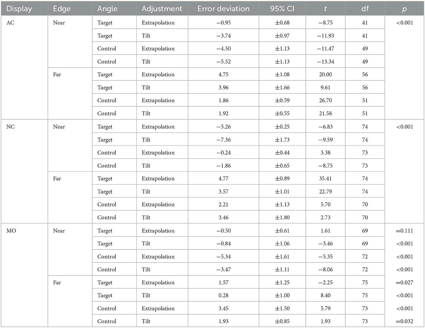
Table 1. Statistical data relevant to the likelihood analysis in Subsection 3.3.2.

In the AC condition, adjustments relative to both far edges were accounted for by the Cluster 1 centroid (2°, 2°), which provided their maximum likelihood estimators. Instead, the maximum likelihood estimators of adjustments relative to near edges were provided by the Cluster 2 centroid (−2°, −4°). Applying Equations 1 and 2, we extracted the errors predicted by a globally consistent solution for near edges using the maximum likelihood estimators of far edges (i.e., the Cluster 1 centroid) and the predicted errors for far edges using the maximum likelihood estimators of near edges (i.e., the Cluster 2 centroid). The resulting adjustment errors were (2°, 2°) for near edges and (−6°, −4°) for far edges. The results of one sample Welch's t-tests revealed that the average distribution of observed extrapolation and tilt errors relative to near edges deviated significantly from errors required by a globally consistent solution. Similarly, the average of the distribution of extrapolation and tilt errors of far edges deviated significantly from the adjustment error predicted by a globally consistent solution.

For the No-completion display, adjustment errors relative to both far edges and to the near edge of the target angle were grouped in Cluster 1 with centroid (1°, 1°) providing their maximum likelihood estimates, whereas the maximum likelihood estimates of the distribution of adjustment errors relative to the near edge of the control angle were grouped by the Cluster 2 centroid (−5°, −8°). These centroids, when recalculated according to Equations 1 and 2, provided the following pair of adjustment errors predicted by a globally consistent solution: (1°, 1°) for adjustments relative to both near edges and to the far edge of the control angle and (−11°, −8°) for adjustments relative to the far edge of the target angle. Again and similarly to the AC condition the results of one sample Welch's t-tests revealed that the observed distribution of extrapolation and tilt errors was far from being globally consistent in all experimental conditions.

As regards the Mosaic display, the adjustment errors required by a globally consistent solution for both the near and the far edge of the control angle were (1°, 1°), as predicted by the Cluster 1 centroid (1°, 1°). The error required on the far edge of the target angle was (−3°, −4°) according to the Cluster 2 centroid (−5°, −4°). These values were not predictive for the great majority of conditions at Welch's t-tests.

4. Discussion

In our study we measured for the first time the orientation of sides of coincidentally occluded angles in the Gerbino illusion display (Gerbino, 1978, 2017, 2020; Da Pos and Zambianchi, 1996), as well as in two control conditions. In the Gerbino illusion display, the coincidental occlusion of a regular hexagon by equilateral triangles leads to a perceived shape distortion often described as a misplacement of the sides of the hexagon. We tested the hypothesis that at least part of this shape distortion involves the misrepresentation of side orientation; i.e., a loss of veridicality possibly associated with the generation of smooth monotonic amodal contours. We found evidence that the concatenation of local distortions induced by the coincidentally occluding triangles determines the perception of a globally misoriented shape, in accordance with the visual approximation framework and previous findings (Fantoni et al., 2007; Gerbino, 2017, 2020).

To measure the perceived orientation of the two sides of a coincidentally occluded angle of the Gerbino illusion display we devised and applied a novel probing technique, based on the sequential adjustment of a dot (extrapolation judgment) and a line (tilt judgment). Results met our expectations. In particular, probe adjustments deviated from the literal representation of input fragments postulated by the visual interpolation framework to AC in two ways: as an effect of coincidental occlusion, the amodally completed angle was shrinked and slightly rotated in the CCW direction, relative to the angle formed by input fragments. This solution is in line with Fantoni et al. (2007).

Coincidental occlusion produced a pattern of local extrapolation and tilt distortions depending on edge type, whether near or far from the coincidentally occluded angle. In particular, errors relative to the edges ending on coincidentally occluded angles (near edge/control angle and near edge/target angle) were opposite in sign (diagnostic of a CW rotation) and globally smaller than errors relative to the corresponding edge of the modal side (far edge/target angle and far edge/control angle). We named this pattern of effects a non-collinear solution with shrinked angle distortion.

Results in the two control conditions differed from those in the experimental AC condition. Probe adjustments suggest that in the No-completion condition (where the fully visible hexagon partially occluded the equilateral triangles) and in the Mosaic condition (where the triangles were indistinguishable from the background and the only shape the fragmentary portion of the hexagon of the experimental AC display was visible) the right side of the target angle was represented veridically, while the left side was strongly distorted in the CW direction. Future research should clarify if the latter distortion is at least partially dependent on the absolute orientation, which in our experiment was very different for left and right sides of the target angle.

The comparison of results from our three Display conditions allowed us to exclude the asymmetric arrangement of triangles and the spiral-like shape of the visually specified portion of the partially occluded hexagon as determinants of the Gerbino illusion. Taken together, our results support the conclusion that in limiting cases of coincidental occlusion, such as the Gerbino illusion display, visual approximation provides a better framework for AC processes than visual interpolation.

In general, our study extends previous evidence on visual approximation in both pictorial (Mussap and Levi, 1995; Fantoni et al., 2005) and 3D domains (Liu et al., 1999; Hou et al., 2006; Fantoni et al., 2008a,b). This evidence suggests that AC processes include the generation of an approximated representation of input fragments driven by smoothness and monotonicity constraints (Fantoni and Gerbino, 2003; Fantoni et al., 2008b; Gerbino, 2017, 2020).

The approximation-based interpretation is also compatible with the original interpretation of the Gerbino illusion within the interpolation framework (Gerbino, 1978). According to visual interpolation, the Gerbino illusion is caused by the irresistible tendency of T-stems toward good continuation, and by the consequent representation of the far edge extrapolation as intersecting the linear extrapolation of the near edge of the other side, without any orientation distortion.

In general, the effects of AC processes on modal parts (discussed by Gerbino, 2020) fit an idea originally proposed by Fantoni et al. (2008a). Amodally completed parts could be generated in parallel with the computation of luminance-defined properties, and modulate them through feedforward interactions (Hoff and Ahuja, 1989; Lee et al., 2002). This possibility calls for the inclusion of AC processes into models of luminance-defined shapes (Marr, 1982; DeAngelis et al., 1991; Grossberg, 1994; Archie and Mel, 2000), with visual approximation being an important computational tool. At the present stage of research, we suggest that visual approximation constitutes a mid-level heuristic supporting the completion of contour fragments. Under coincidental occlusion conditions, this heuristic might imply the misrepresentation of contour orientation.

Though overlooked by the mainstream approach to AC, visual approximation deserves further investigation as a process capable of explaining a broader range of pictorial and 3D phenomena than visual interpolation alone. An important aspect to investigate concerns the conditions under which non-collinear fragments are distorted to generate a smooth and monotonic connection between them. It is reasonable to expect that the tendency to distort non-collinear fragments under coincidental occlusion conditions would be comparatively reduced as the turning angle between fragments gets smaller. Increasing the convergence between visually approximated fragments would indeed reach the limits for visual approximation to occur (90° relatability constraint). Studying this constraint to visual approximation would be fundamental to shed light on the image geometry supporting AC, and in particular on the limits beyond which fragments are perceived as unconnected.

Data availability statement

The original contributions presented in the study are included in the article/Supplementary material, further inquiries can be directed to the corresponding author.

Ethics statement

The studies involving humans were approved by Research Ethics Committee of the University of Trieste (Approval Number: 84c/2017). The studies were conducted in accordance with the local legislation and institutional requirements. The participants provided their written informed consent to participate in this study.

Author contributions

CF and WG conceived the original idea. AD carried out the experiment and wrote the first draft. AD and CF contributed to data analysis. All authors discussed the results and contributed to the final manuscript and revision.

Funding

This work was supported by a research grant to CF (RESRIC-FANTONI2018, Department of Life Sciences, University of Trieste).

Conflict of interest

The authors declare that the research was conducted in the absence of any commercial or financial relationships that could be construed as a potential conflict of interest.

Publisher's note

All claims expressed in this article are solely those of the authors and do not necessarily represent those of their affiliated organizations, or those of the publisher, the editors and the reviewers. Any product that may be evaluated in this article, or claim that may be made by its manufacturer, is not guaranteed or endorsed by the publisher.

Supplementary material

The Supplementary Material for this article can be found online at: https://www.frontiersin.org/articles/10.3389/fcogn.2023.1216459/full#supplementary-material

Footnotes

1. ^By coincidental occlusion we mean the limiting condition in which the edge of an occluding surface lies exactly on the vertex of a partially occluded angle, such that the foreground surface partially occludes only one of the two angle's sides while leaving the other completely unoccluded.

2. ^T-stem and T-top are the conventional labels for the two segments of a T-junction, referring to vertical and horizontal segments of a normally oriented T, respectively. Far and near labels are relative to the vertex shared by the two edges; every side of the hexagon in Figures 1C, D plays both roles (far edge and near edge) with respect to different adjacent vertices. Since the Gerbino illusion is reduced when the far edge is either vertical or horizontal, all hexagons in our study were shown in the oblique orientation illustrated in Figure 1.

3. ^Ground continuation can lead to the illusion of absence (Svalebjørg et al., 2020), like in the famous court scene that Koffka (1935, p. 180) included in the paragraph of the Principles of Gestalt psychology where AC, well before getting its present name, was appropriately called “representation without colour” (Koffka, 1935, p. 178).

4. ^Smoothness and monotonicity constraints are also embodied in relatability theory (Kellman and Shipley, 1991). However, since this theory includes further assumptions—namely, the 90° constraint—we will use “connectable”—instead of “relatable”—for contour fragments that can be joined along a smooth monotonic path (Fantoni and Gerbino, 2013).

5. ^At least three expressions are used in the literature to express the same concept: genericity principle, generic viewpoint assumption, generic view principle. In the case of a coincidentally occluded angle, all refer to the following constraint to image interpretation: to comply with the genericity principle, the shape of the amodally completed angle should not conflict with images associated to slight perturbations of the viewpoint which can reveal a contour discontinuity. In the present paper, the notion of genericity is used also with a different meaning. Referring to occlusion geometry, an angle is occluded in a generic (rather than coincidental, or accidental) way if the viewpoint, the occluding edge and the angle's vertex are not aligned.

6. ^Unfortunately, the conference abstract in Fantoni et al. (2007) did not illustrate the obtained results clearly. See Fantoni et al. (2008a, end of Subsection 3) for the correct description of the direction of global rotation.

7. ^We used a technique in which observers adjusted probes without changing any feature of the target display that elicits the distortion under study. Techniques based on nulling, like the one utilized by Gerbino (1978), can provide relevant information about the illusion, but imply undesirable changes of the target display.

8. ^In the No-completion condition the circular probe paths were the same as in the other two conditions, making impossible to maintain constant the probe-endpoint distance.

9. ^The simple misorientation of the near edge (while representing the position of the vertex and the whole far edge veridically) would imply a misrepresentation of angle size but not solve the problem posed by its coincidental occlusion.

10. ^Errors might occur in the opposite CW direction if they were corresponding to the output of the second stage of AC processes, as revealed—for instance—by the explicit extrapolation task utilized by Gerbino (1978).

References

Albert, M. K. (2001). Surface perception and the generic view principle. Trends Cogn. Sci. 5, 197–203. doi: 10.1016/S1364-6613(00)01643-0

PubMed Abstract | CrossRef Full Text | Google Scholar

Albert, M. K., and Hoffman, D. D. (1995). “Genericity in spatial vision,” in Geometric Representations of Perceptual Phenomena: Papers in Honor of Tarow Indow's 70th Birthday, ed D. Luce (Mahwah, NJ: Erlbaum), 95–112.

Google Scholar

Archie, K. A., and Mel, B. W. (2000). A model for intradendritic computation of binocular disparity. Nat. Neurosci. 3, 54–63. doi: 10.1038/71125

PubMed Abstract | CrossRef Full Text | Google Scholar

Attneave, F. (1954). Some informational aspects of visual perception. Psychol. Rev. 61, 183–193. doi: 10.1037/h0054663

PubMed Abstract | CrossRef Full Text | Google Scholar

Barr, D. J., Levy, R., Scheepers, C., and Tily, H. J. (2013). Random effects structure for confirmatory hypothesis testing: keep it maximal. J. Mem. Lang. 68, 255–278. doi: 10.1016/j.jml.2012.11.001

PubMed Abstract | CrossRef Full Text | Google Scholar

Ben-Shahar, O., and Zucker, S. (2004). Geometrical computations explain projection patterns of long-range horizontal connections in visual cortex. Neural Comput. 16, 445–476. doi: 10.1162/089976604772744866

PubMed Abstract | CrossRef Full Text | Google Scholar

Breckon, T. P., and Fisher, R. B. (2005). Amodal volume completion: 3D visual completion. Comput. Vis. Image Understand. 99, 499–526. doi: 10.1016/j.cviu.2005.05.002

CrossRef Full Text | Google Scholar

Burke, L. (1952). On the tunnel effect. Quart. J. Exp. Psychol. 4, 121–138. doi: 10.1080/17470215208416611

CrossRef Full Text | Google Scholar

Charrad, M., Ghazzali, N., Boiteau, V., and Niknafs, A. (2014). NbClust: an R package for determining the relevant number of clusters in a data set. J. Stat. Softw. 61, 1–36. doi: 10.18637/jss.v061.i06

CrossRef Full Text | Google Scholar

Da Pos, O., and Zambianchi, E. (1996). Illusioni ed effetti visivi. Una raccolta (Visual Illusions and Effects. A Collection). Milan: Guerini e Associati.

Google Scholar

DeAngelis, G. C., Ohzawa, I., and Freeman, R. D. (1991). Depth is encoded in the visual cortex by a specialized receptive field structure. Nature 352, 156–159. doi: 10.1038/352156a0

PubMed Abstract | CrossRef Full Text | Google Scholar

Ekroll, V., Mertens, K., and Wagemans, J. (2018). Amodal volume completion and the thin building illusion. i-Perception 9, 1–21. doi: 10.1177/2041669518781875

PubMed Abstract | CrossRef Full Text | Google Scholar

Ekroll, V., Sayim, B., and Wagemans, J. (2017). The other side of magic: the psychology of perceiving hidden things. Perspect. Psychol. Sci. 12, 91–106. doi: 10.1177/1745691616654676

PubMed Abstract | CrossRef Full Text | Google Scholar

Elder, J. H., and Goldberg, R. M. (2002). Ecological statistics of Gestalt laws for the perceptual organization of contours. J. Vis. 2, 5. doi: 10.1167/2.4.5

PubMed Abstract | CrossRef Full Text | Google Scholar

Fantoni, C., Bertamini, M., and Gerbino, W. (2005). Contour curvature polarity and surface interpolation. Vis. Res. 45, 1047–1062. doi: 10.1016/j.visres.2004.10.023

PubMed Abstract | CrossRef Full Text | Google Scholar

Fantoni, C., and Gerbino, W. (2003). Contour interpolation by vector-field combination. J. Vis. 3, 4. doi: 10.1167/3.4.4

PubMed Abstract | CrossRef Full Text | Google Scholar

Fantoni, C., and Gerbino, W. (2013). “Connectability” matters too: completion theories need to be complete. Cogn. Neurosci. 4, 47–48. doi: 10.1080/17588928.2012.748022

PubMed Abstract | CrossRef Full Text | Google Scholar

Fantoni, C., Gerbino, W., and Kellman, P. J. (2008a). Approximation, torsion, and amodally-unified surfaces. J. Vis. 4, 726. doi: 10.1167/4.8.726

CrossRef Full Text | Google Scholar

Fantoni, C., Gerbino, W., and Rigutti, S. (2007). Form Misorientation in Limiting Cases of Amodal Completion. ECVP 2007. 36, 106.

Google Scholar

Fantoni, C., Hilger, J. D., Gerbino, W., and Kellman, P. J. (2008b). Surface interpolation and 3D relatability. J. Vis. 8, 29. doi: 10.1167/8.7.29

PubMed Abstract | CrossRef Full Text | Google Scholar

Faul, F., Erdfelder, E., Lang, A.-G., and Buchner, A. (2007). G^*Power 3: a flexible statistical power analysis program for the social, behavioral, and biomedical sciences. Behav. Res. Methods 39, 175–191. doi: 10.3758/BF03193146

PubMed Abstract | CrossRef Full Text | Google Scholar

Field, D. J., Hayes, A., and Hess, R. F. (1993). Contour integration by the human visual system: evidence for a local “association field”. Vis. Res. 33, 173–193. doi: 10.1016/0042-6989(93)90156-Q

PubMed Abstract | CrossRef Full Text | Google Scholar

Fulvio, J. M., Singh, M., and Maloney, L. T. (2008). Precision and consistency of contour interpolation. Vis. Res. 48, 831–849. doi: 10.1016/j.visres.2007.12.018

PubMed Abstract | CrossRef Full Text | Google Scholar

Geisler, W. S., Perry, J. S., Super, B. J., and Gallogly, D. P. (2001). Edge co-occurrence in natural images predicts contour grouping performance. Vis. Res. 41, 711–724. doi: 10.1016/S0042-6989(00)00277-7

PubMed Abstract | CrossRef Full Text | Google Scholar

Gerbino, W. (1978). Some observations on the formation of angles in amodal completion. Ital. J. Psychol. 5, 85–100.

Google Scholar

Gerbino, W. (2017). “Amodally completed angles,” in The Oxford Compendium of Visual Illusions, eds A. G. Shapiro and D. Todorović (Oxford: Oxford University Press), 673–678. doi: 10.1093/acprof:oso/9780199794607.003.0097

PubMed Abstract | CrossRef Full Text | Google Scholar

Gerbino, W. (2020). Amodal completion revisited. i-Perception 11, 2041669520937323. doi: 10.1177/2041669520937323

PubMed Abstract | CrossRef Full Text | Google Scholar

Gerbino, W., and Fantoni, C. (2006). Visual interpolation is not scale invariant. Vis. Res. 46, 3142–3159. doi: 10.1016/j.visres.2006.03.030

PubMed Abstract | CrossRef Full Text | Google Scholar

Gerbino, W., Scomersi, S., and Fantoni, C. (2006). Amodal completion enhances the discrimination of Vernier offset. J. Vis. 6, 99–99. doi: 10.1167/6.6.99

CrossRef Full Text | Google Scholar

Gerbino, W., and Zabai, C. (2003). The joint. Acta Psychol. 114, 331–353. doi: 10.1016/j.actpsy.2003.10.002

PubMed Abstract | CrossRef Full Text | Google Scholar

Germine, L., Nakayama, K., Duchaine, B. C., Chabris, C. F., Chatterjee, G., and Wilmer, J. B. (2012). Is the Web as good as the lab? Comparable performance from Web and lab in cognitive/perceptual experiments. Psychon. Bullet. Rev. 19, 847–857. doi: 10.3758/s13423-012-0296-9

PubMed Abstract | CrossRef Full Text | Google Scholar

Grossberg, S. (1994). 3-D vision and figure-ground separation by visual cortex. Percept. Psychophys. 55, 48–121. doi: 10.3758/BF03206880

PubMed Abstract | CrossRef Full Text | Google Scholar

Hoff, W., and Ahuja, N. (1989). Surfaces from stereo: integrating feature matching, disparity estimation, and contour detection. IEEE Trans. Pat. Anal. Machine Intell. 11, 121–136. doi: 10.1109/34.16709

CrossRef Full Text | Google Scholar

Horn, B. K. P. (1983). The curve of least energy. ACM Trans. Math. Softw. 9, 441–460. doi: 10.1145/356056.356061

CrossRef Full Text | Google Scholar

Hotopf, W. H. N., Ollerearnshaw, C., and Brown, S. (1974). The regression to right angles tendency and the Poggendorff illusion. Br. J. Psychol. 65, 213–231. doi: 10.1111/j.2044-8295.1974.tb01396.x

PubMed Abstract | CrossRef Full Text | Google Scholar

Hou, F., Lu, H., Zhou, Y., and Liu, Z. (2006). Amodal completion impairs stereoacuity discrimination. Vis. Res. 46, 2061–2068. doi: 10.1016/j.visres.2005.12.010

PubMed Abstract | CrossRef Full Text | Google Scholar

Kanizsa, G. (1955). “Margini quasi-percettivi in campi con stimolazione omogenea. Rivista di psicologia. 49, 7–30. English translation: Quasi-perceptual margins in homogeneously stimulated fields,” in The Perception of Illusory Contours, eds S. Petry and G. E. Meyer (New York, NY: Springer), 40–49. doi: 10.1007/978-1-4612-4760-9_4

CrossRef Full Text | Google Scholar

Kanizsa, G. (1979). Organization in Vision. New York, NY: Praeger.

Google Scholar

Kanizsa, G., and Gerbino, W. (1982). “Amodal completion: seeing or thinking?,” in Organization and Representation in Perception, ed J. Beck (Mahwah, NJ: Erlbaum), 167–190.

Google Scholar

Kellman, P. J., Garrigan, P., and Shipley, T. F. (2005). Object interpolation in three dimensions. Psychol. Rev. 112, 586–609. doi: 10.1037/0033-295X.112.3.586

PubMed Abstract | CrossRef Full Text | Google Scholar

Kellman, P. J., and Shipley, T. F. (1991). A theory of visual interpolation in object perception. Cogn. Psychol. 23, 141–221. doi: 10.1016/0010-0285(91)90009-D

PubMed Abstract | CrossRef Full Text | Google Scholar

Koffka, K. (1935). Principles of Gestalt Psychology. New York, NY: Harcourt Brace.

Google Scholar

Lee, M.-S., Medioni, G., and Mordohai, P. (2002). Inference of segmented overlapping surfaces from binocular stereo. IEEE Trans. Pat. Anal. Machine Intell. 24, 824–837. doi: 10.1109/TPAMI.2002.1008388

CrossRef Full Text | Google Scholar

Leeuwenberg, E., and Van der Helm, P. A. (2013). Structural Information Theory: The Simplicity of Visual Form. Cambridge: Cambridge University Press.

PubMed Abstract | Google Scholar

Liu, Z., Jacobs, D. W., and Basri, R. (1999). The role of convexity in perceptual completion: beyond good continuation. Vis. Res. 39, 4244–4257. doi: 10.1016/S0042-6989(99)00141-8

PubMed Abstract | CrossRef Full Text | Google Scholar

Marr, D. (1982). Vision: A Computational Investigation into the Human Representation and Processing of Visual Information. San Francisco, CA: Freeman.

Google Scholar

Michotte, A., and Burke, L. (1951). Une nouvelle enigme de la psychologie de la perception: le “donnee amodal” dans l'experience sensorielle [A new enigma in the psychology of perception: The “amodally given” in the sensory experience],” in Actes du XIII Congres Internationale de Psychologie, eds A. Michotte et collaborateurs and V. Ferri (Louvain: Publications Universitaires de Louvain), 179–180.

Google Scholar

Michotte, A., Thinès, G., and Crabbé, G. (1964). Les complements amodaux des structures perceptives. Louvain: Publications Universitaires de Louvain.

PubMed Abstract | Google Scholar

Mussap, A. J., and Levi, D. M. (1995). Amodal completion and vernier acuity: evidence of ‘top-but-not-very-far-down' processes? Perception 24, 1021–1048. doi: 10.1068/p241021

PubMed Abstract | CrossRef Full Text | Google Scholar

Ninio, J. (2014). Geometrical illusions are not always where you think they are: a review of some classical and less classical illusions, and ways to describe them. Front. Hum. Neurosci. 8, 856. doi: 10.3389/fnhum.2014.00856

PubMed Abstract | CrossRef Full Text | Google Scholar

Palmer, S. E. (1999). Vision Science: Photons to Phenomenology. Cambridge, MA: MIT Press.

Google Scholar

Palmer, S. E., Brooks, J. L., and Lai, K. S. (2007). The occlusion illusion: partial modal completion or apparent distance? Perception 36, 650–669. doi: 10.1068/p5694

PubMed Abstract | CrossRef Full Text | Google Scholar

Palmer, S. E., and Schloss, K. B. (2017). “The occlusion, configural shape, and shrinkage illusions,” in The Oxford Compendium of Visual Illusions, eds A. G. Shapiro and D. Todorović (Oxford: Oxford University Press), 269–274. doi: 10.1093/acprof:oso/9780199794607.003.0029

PubMed Abstract | CrossRef Full Text | Google Scholar

Pinna, B. (2012). The role of amodal completion in shape formation: some new shape phenomena. Perception 41, 1336–1354. doi: 10.1068/p7331

PubMed Abstract | CrossRef Full Text | Google Scholar

Robinson, J. O. (1972). The Psychology of Visual Illusions. London: Hutchinson.

Google Scholar

Rock, I. (1983). The Logic of Perception. Cambridge: MIT Press.

Google Scholar

Rubin, E. (1921). Visuell wahrgenommene Figuren: Studien in psychologischer Analyse. Kobenhaven: Gyldendal.

Google Scholar

Scherzer, T. R., and Ekroll, V. (2015). Partial modal completion under occlusion: what do modal and amodal percepts represent? J. Vis. 15, 22–22. doi: 10.1167/15.1.22

PubMed Abstract | CrossRef Full Text | Google Scholar

Singh, M., and Hoffman, D. D. (1999). Completing visual contours: the relationship between relatability and minimizing inflections. Percept. Psychophys. 61, 943–951. doi: 10.3758/BF03206908

PubMed Abstract | CrossRef Full Text | Google Scholar

Svalebjørg, M., Øhrn, H., and Ekroll, V. (2020). The illusion of absence in magic tricks. i-Perception 11, 2041669520928383. doi: 10.1177/2041669520928383

PubMed Abstract | CrossRef Full Text | Google Scholar

Takeichi, H., Nakazawa, H., Murakami, I., and Shimojo, S. (1995). The theory of the curvature-constraint line for amodal completion. Perception 24, 373–389. doi: 10.1068/p240373

PubMed Abstract | CrossRef Full Text | Google Scholar

Tse, P. U. (1999). Volume completion. Cogn. Psychol. 39, 37–68. doi: 10.1006/cogp.1999.0715

PubMed Abstract | CrossRef Full Text | Google Scholar

Ullman, S. (1976). Filling-in the gaps: the shape of subjective contours and a model for their generation. Biol. Cybernet. 25, 1–6. doi: 10.1007/BF00337043

CrossRef Full Text | Google Scholar

van Lier, R., and Gerbino, W. (2015). “Perceptual completions,” in The Oxford Handbook of Perceptual Organization, ch. 15, ed J. Wagemans (Oxford: Oxford University Press), 304–330. doi: 10.1093/oxfordhb/9780199686858.013.040

CrossRef Full Text | Google Scholar

van Lier, R., van der Helm, P., and Leeuwenberg, E. (1995). Competing global and local completions in visual occlusion. J. Exp. Psychol. 21, 571–583. doi: 10.1037/0096-1523.21.3.571

PubMed Abstract | CrossRef Full Text | Google Scholar

Vezzani, S. (1999). Shrinkage and expansion by amodal completion: a critical review. Perception 28, 935–947. doi: 10.1068/p280935

PubMed Abstract | CrossRef Full Text | Google Scholar

Weintraub, D. J., and Krantz, D. H. (1971). The Poggendorff illusion: amputations, rotations, and other perturbations. Percept. Psychophys. 10, 257–264. doi: 10.3758/BF03212818

CrossRef Full Text | Google Scholar

Wertheimer, M. (1923). Untersuchungen zur Lehre von der Gestalt. II. Psychologische Forschung 4, 301–350. doi: 10.1007/BF00410640

CrossRef Full Text | Google Scholar