Segmentation of tooth enamel microstructure images using classical image processing and U-Net approaches

1. Introduction

Tooth enamel is the most highly mineralized tissue (95% of mineral) in an organism and is able to withstand high temperatures, abrasion, aggressive environments (i.e., humidity, pressure), and degradation over time (Sweet and Sweet, 1995; Valenzuela et al., 2000). These characteristics have proved to be beneficial for human identification in massive disasters, such as when victims were carbonized at high temperatures and visual or fingerprint identification was no longer possible (Valenzuela et al., 2000).

Most mammalians, including humans, present with tooth enamel composed of layers of prisms regularly arranged in alternating directions nearly perpendicular to each other (von Koenigswald et al., 1987). These prisms act like optic fibers when exposed to a direct light source (Whittaker and Rothwell, 1984) and form Hunter–Schreger Bands (HSBs), an optical phenomenon that appears as light and dark stripes on the tooth's surface and can be seen with a magnifier when a low-power light is placed to the side of the tooth (Koenigswald, 1994). A thorough analysis of HSBs may provide information regarding a species' life history and taxon identification (Line and Bergqvist, 2005) since it is frequently preserved in tooth fossils dating from thousands to over 60 million years (Koenigswald, 1994), can be used for inferences about diet adaptation (Tseng, 2012), and provide data for biometric identification (Ramenzoni and Line, 2006).

Biometric analysis is the process of personal identification using the biological, physical, or behavioral features of an individual. Currently, there are several biometric methods, including facial, iris, fingerprint, ear, and gait recognition. These methods are applied using automated systems and software that can be used to distinguish individuals reliably. Some desirable characteristics of biometrics data are their being highly unique, easily obtainable, time-invariant (no significant changes over time), easily transmittable, non-intrusively acquirable, and distinguishable by humans without special training (Shen and Tan, 1999). Previous work has shown that a photograph of a tooth with side lighting enhances the HSB appearance (Arrieta and Line, 2017) and that a digital image of HSBs can be treated to highlight the bands (Arrieta et al., 2018). The light and dark patterns formed by the HSBs resemble fingerprints and seem to be unique for each tooth and between individuals (Ramenzoni and Line, 2006). Moreover, tooth image acquisition is non-invasive and practical and can be obtained with a photographic camera using a macro lens.

To be used as a human identification method, as opposed to fingerprints, HSB features cannot be extracted directly from sensors because they are only visible with side illumination. A problem in the image processing of HSBs is the removal of background image areas, including areas of the tooth with poorly defined bands and areas outside of the tooth. These regions can interfere with digital image filtering and produce false HSB patterns. Although these areas can be manually removed, this process is not reliable since the selected areas can vary according to the individual's subjective perception. In addition, it is also a time-consuming procedure. Therefore, the aim of the present project is to develop software that automatically selects the region of interest (ROI), that is, the HSB region whose bands are reliable for biometric comparison, thus making the entire process straightforward.

The workflow for the whole biometric process is illustrated in Figure 1. The segmentation approaches presented here were built to create a proper mask to segment the HSB region, which in turn will be enhanced by an HSB filter and eventually pass through biometric feature extraction for either storage as a template or comparison for personal identification. Note that for real applications, tooth photographs should be taken at the tooth crown level in the mouth. Therefore, anterior teeth are preferred for ease of access. In the present study, we evaluated the techniques for segmentation in extracted teeth but with a similar potential for in-mouth applications.

FIGURE 1

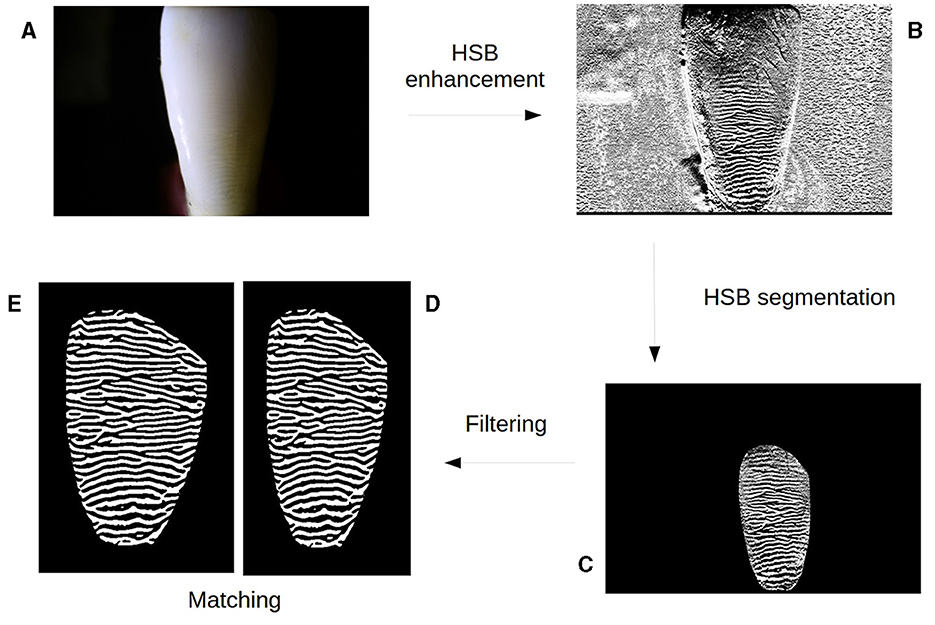
Figure 1. Tooth biometrics workflow. The workflow starts with original photography of tooth crown under side lighting (A) that goes through a Hunter-Schreger Band (HSB) enhancement (Arrieta et al., 2018). Then, the reliable enhanced HSB (B) is segmented (C) and filtered into a binary noiseless image representing the tooth HSB pattern (D), which in turn might be stored as template or be compared against tooth templates registered in a database (E) using a matching algorithm.

2. Methods

In this section, we present the methods that were developed to automatically segment the HSBs. The teeth used in this study were provided by the Biobank of Bones, Teeth and Human Corpses of the Department of Biosciences of the Piracicaba Dental School. This study was approved by the research ethics committee of the Piracicaba Dental School under number CAAE 03596918.2.0000.5418. We considered two approaches, classical image processing and a convolutional neural network, for automatic segmentation. The first one is an image processing pipeline based on the anisotropic HSB property. The second one is known as U-Net, a fully convolutional neural network created for medical image segmentation (Ronneberger et al., 2015).

2.1. Anisotropy-based segmentation

The anisotropy-based segmentation (ABS) approach takes advantage of the well-established orientation pattern of HSBs, in addition to their relatively low variation in orientation. Once the tooth photograph is taken with the tooth vertically positioned, its bands consequently will appear horizontally overall. Therefore, it is unnecessary to apply any rotation. The physical property of an object that presents different values according to measures along different axes is called anisotropy. This property arises mainly in the regions of the image containing HSB patterns, and harnessing this characteristic for segmenting the area of interest is possible due to (1) anisotropic features around a tooth are very unlikely to exist, except for the HSBs of its neighboring teeth; (2) the focus of the camera on the HSB pattern of the targeted tooth surface makes other regions blurry; and (3) the HSBs appear only under side lighting, and the residual light effect on neighboring teeth is expected to be weaker. The ABS workflow is shown in Figure 2. A complete description follows. All parameter values chosen were validated across the available data set using the visualization method described by Fogalli et al. (2022).

FIGURE 2

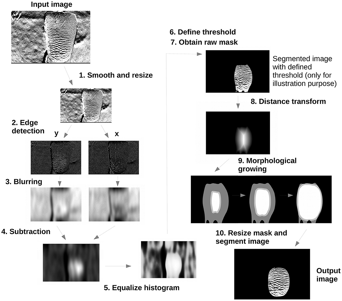
Figure 2. Anisotropy-based segmentation workflow.

2.1.1. Smooth and resize

The primary goal of this processing step is to standardize image features before further processing, given the variations present in the input images. Since the initial and enhanced HSB images are noisy, high-resolution images, and the segmentation process do not require these levels of detail; we start the process by smoothing the enhanced HSB image E into E_s such as

$\begin{array}{ll}{E}_s=W_{(27,27)}\star E,& (1)\end{array}$

where W_{(27, 27)} represents a 27 × 27 integral kernel (whose sum equals 1) and the star sign (⋆) represents a cross-correlation between the kernel and the image E. The expanded version of this expression is demonstrated as follows: Let a be a kernel with size (2h+1) × (2w+1) and B an image; the cross-correlation between them can be computed with

$\begin{array}{ll}a\star B(i,j)={\displaystyle \sum _{u=-h}^h}{\displaystyle \sum _{v=-w}^w}a(u,v)·B(u+i,j+v).& (2)\end{array}$

The ROI seems to follow roughly the shape of the tooth crown. Since anterior teeth are preferable, we assumed its dimensions as default. Consider a front image of an anterior tooth vertically positioned, its frontal surface has a vertical dimension greater than the horizontal dimension at tooth's neck, that is, where the HSBs appear more clearly due to a thinner enamel layer, so the ROI usually is taller vertically and thinner horizontally (Figure 3). Hence, after visual comparisons of the algorithm results using proportions of width over height from 1 (square shape) to $\frac{1}{5}$, the chosen and validated proportion for ROI was set to $\frac{1}{2}$.

FIGURE 3

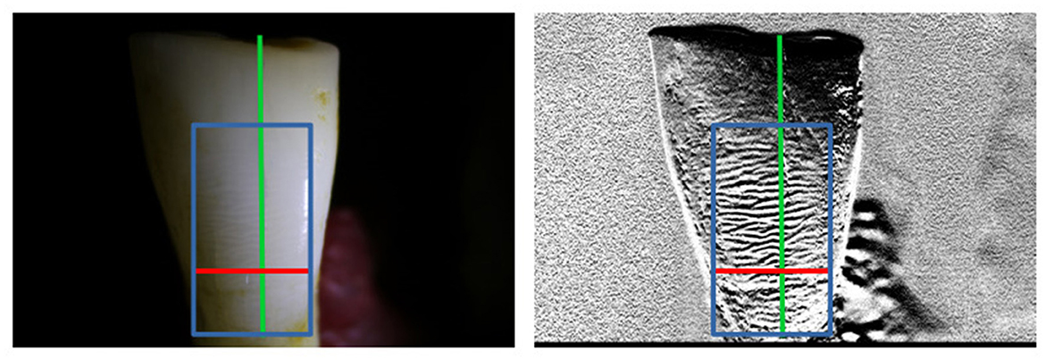
Figure 3. Original photography and enhanced Hunter–Schreger Band (HSB) image of an anterior tooth with proportion measures. Green line is the vertical size of the tooth crown. Red line is the horizontal measure of the tooth frontal surface. Blue box represents approximately the extension of recoverable HSB (region of interest).

In order to maximize performance and standardize the segmentation process, the HSB-enhanced grayscale image E_s with dimensions of M rows and N columns (M×N) is resized to image J of dimensions P×Q according to the following equations:

$\begin{array}{ll}\text{P}=r\text{Q},& (3)\end{array}$

$\begin{array}{ll}r=\frac{\text{M}}{\text{N}},& (4)\end{array}$

$\begin{array}{ll}\text{Q}=\sqrt{\frac{J_{size}}{r}},& (5)\end{array}$

$\begin{array}{ll}{J}_{size}=\text{P}\text{Q}=k_x{k}_{y}u,& (6)\end{array}$

where parameter u was empirically determined by visually comparing the results for different possible values and validated afterward. It is also proportional to the new desired image size; we used u = 200 as default. The scalars k_x = 61 and k_y = 122 are related to a kernel filter size that will be used later, and their values were chosen accordingly to fit the ROI proportion $\frac{k_x}{k_y}=\frac{1}{2}$. With those settings, the size of image J is fixed at $J_{size}=1.5\times 10^6$ pixels. Let image J_b be the blurred version of J, computed as

$\begin{array}{ll}{J}_b=W_{(3,6)}\star (W_{(3,6)}\star (W_{(3,6)}\star J)),& (7)\end{array}$

where W_{(3, 6)} is a 3 × 6 integral kernel. Kernel shape and size were selected using the validation approach described previously by Fogalli et al. (2022) for determining other parameters. The horizontally elongated kernel reduces the noise in the background that could mimic HSB edges, mainly in regions of the tooth with artifacts from reflected light, while causing virtually no disturbance to the real HSB.

2.1.2. Edge detection

The HSBs are expected to appear as horizontal stripes. In this processing step, horizontal and vertical edges are detected, hinting at regions containing horizontal stripes (HSBs) or not, respectively. Therefore, after obtaining image J_b, we decompose its features into x and y directions to initially locate the HSB region. Edge detection is performed using horizontal $s_x=\left[\begin{array}{ccc}-1& 0& 1\\ -2& 0& 2\\ -1& 0& 1\\ \end{array}\right]$and vertical $s_y=\left[\begin{array}{ccc}-1& -2& -1\\ 0& 0& 0\\ 1& 2& 1\\ \end{array}\right]$ Sobel operators:

$\begin{array}{ll}{G}_x=s_x\star J_b,& (8)\end{array}$

$\begin{array}{ll}{G}_y=s_y\star J_b.& (9)\end{array}$

The filtered image G_y highlights, among other possible undesirable horizontal features, the HSB region. While the filtered image G_x highlights regions where vertical structures are predominant. To remove high-frequency gradients mostly represented by noise and keep values in a standardized range, we clip the edge maps to be in [0, 255], such as

$\begin{array}{ll}{G}_{x+}(i,j)=\{\begin{array}{l}0if{G}_x(i,j)<0\\ 255if{G}_x(i,j)>255\\ G_x(i,j)otherwise\end{array},& (10)\end{array}$

$\begin{array}{ll}{G}_{y+}(i,j)=\{\begin{array}{l}0if{G}_y(i,j)<0\\ 255if{G}_y(i,j)>255\\ G_y(i,j)otherwise\end{array}.& (11)\end{array}$

2.1.3. Blurring

The previous step detected edge intensities locally for orthogonal directions (x and y). The edge blurring applied in this step will allow the detection of larger regions in which a preferred edge orientation is present. The blurring will diffuse the edge magnitude equally to their neighborhood and single strong edges (usually not part of HSBs) are mitigated. Once the edges are detected, after blurring them, the regions with concentrated, stronger edges tend to form blobs, whereas sparse and weak-edged regions tend to disappear. Considering that HSBs are confined to a single region in G_y, after blurring its edges, a few blobs are created, and the most intense values appear near the core of the ROI. To perform this, let K be a unit-integral filter kernel of dimensions k_y×k_x, such as

$\begin{array}{ll}K=\left[\begin{array}{ccc}{1}_{(1,1)}& \cdots & 1_{(1,k_x)}\\ ⋮& \ddots & \\ 1_{(k_y,1)}& & 1_{(k_y,k_x)}\end{array}\right]\times \frac{1}{k_y{k}_x}.& (12)\end{array}$

Both images G_x and G_y are filtered again by three repeated cross-correlations with K, resulting, respectively, in the blurred images

$\begin{array}{ll}{B}_x=K\star (K\star (K\star G_{x+})),& (13)\end{array}$

$\begin{array}{ll}{B}_y=K\star (K\star (K\star G_{y+})).& (14)\end{array}$

The shape and size of kernel K are directly related to the level of blurring desired and, consequently, the capture of the details of the ROI shape. A larger K results in heatmaps (described in next section) with more rounded borders, while a smaller K results in more jagged borders (Figure 4). The more cross-correlation repetitions, the larger and longer the area because the number of rows in K is greater than the number of columns. The number of repetitions, that is, three, was chosen after a visual comparison of the general overlap between the ground truth (ROI) and the automated segmented images among all sets and cannot be replaced by a single cross-correlation with a larger kernel size.

FIGURE 4

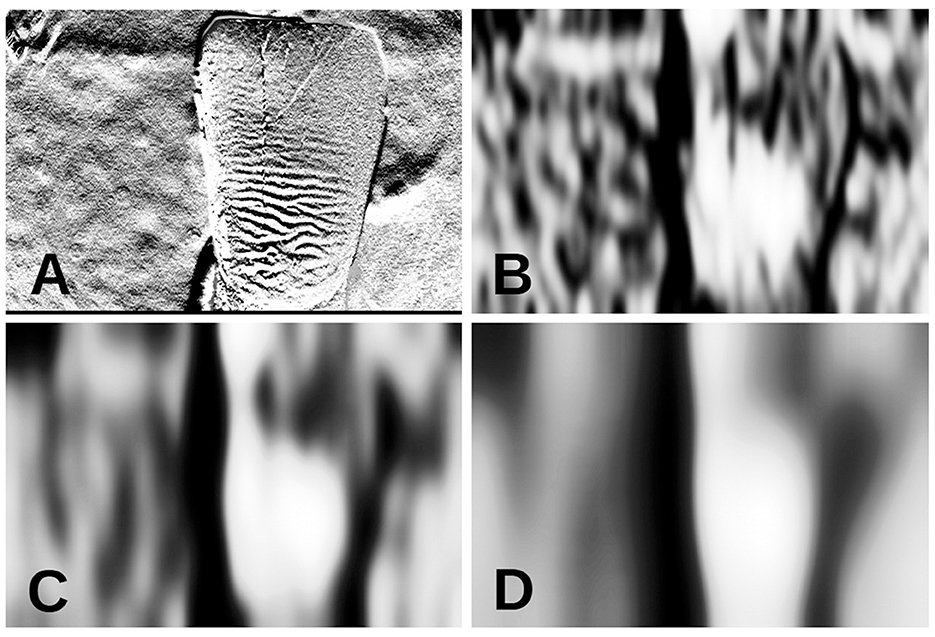
Figure 4. Differences on heatmap H₁ according to parameterizations. (A) Resized tooth image J for segmentation. (B) Heatmap with low parameters k_x = 25 and k_y = 75. (C) Heatmap with intermediate parameters k_x = 50 and k_y = 150. (D) Heatmap with high parameters k_x = 100 and k_y = 300. All images have the same size, achieved by maintaining $J_{size}=1.5\times 10^6$.

2.1.4. Subtraction

Following the previous step in which regions with preferred edge directions (x and y) were accentuated, subtracting one blurred-edge image from the other will result in a map of anisotropy density. Blurred images B_x and B_y represent blurred-edge maps with gradients for horizontal and vertical features, respectively. Subtracting one from the other creates a heatmap in which isotropic regions have values around zero, high values match the locations of the first-term high values, and low values match the locations of the second-term high values. Therefore, with B_y as the first term, the highest values of the heatmap will indicate the ROI. Let the heatmap H₁ for HSB location at position (i, j) be

$\begin{array}{ll}{H}_1(i,j)=B_y(i,j)-2B_x(i,j),& (15)\end{array}$

where B_x is subtracted twice to compensate for the J→J_b (Equation 7), where horizontally detected edges were faded twice as much as vertical ones. Then, from H₁, we remove negative values as follows:

$\begin{array}{ll}{H}_2(i,j)=\{\begin{array}{l}0if{H}_1(i,j)<0\\ H_1(i,j)otherwise\end{array},& (16)\end{array}$

in which H₂ pixel values are in the interval ℝ_p = [0, p], where p varies among different images, depending on the extension and intensity of HSBs produced by the lighted tooth.

2.1.5. Equalize histogram

Since the range of gray-level values vary among different H₂ heatmap samples, an equalized heatmap H₃ is created to normalize grayscale values for the automated process. Hence, let the function γ be

$\begin{array}{ll}\gamma (m_b)=\frac{n_b}{J_{size}},& (17)\end{array}$

where m_b is the bth gray level and n_b is the number of pixels in heatmap H₂ taking the value m_b. The equalized-histogram heatmap H₃ consists of the transformation mapping H₃:ℝ_p → {0, 255} for all b gray levels in H₂. So, the equalized-histogram heatmap H₃ at all positions with pixel value m_b can be defined as

$\begin{array}{ll}{H}_3(m_b)=\lfloor 255{\displaystyle \sum _{a=0}^b}\gamma (m_a)\rceil .& (18)\end{array}$

2.1.6. Define threshold

Since the image gradient of H₃ tends to increase in the direction of the center of the ROI, descending this gradient leads to its borders (Figure 5A). The threshold for the lower bound determines to what extent the HSBs are enclosed. A fixed threshold for enclosing ROI as a foreground mask was tested on a few images without success. Consequently, an adaptive threshold was created based on histogram distribution indexes where large gaps (absence of discrete grayscale values) at high indexes of the histogram are selected as the threshold. To do so, let β be an ordered set of gray levels m_a in H₃, such that

$\begin{array}{ll}\beta =\left\{m_a\mid \gamma (m_a)>0\right\}.& (19)\end{array}$

FIGURE 5

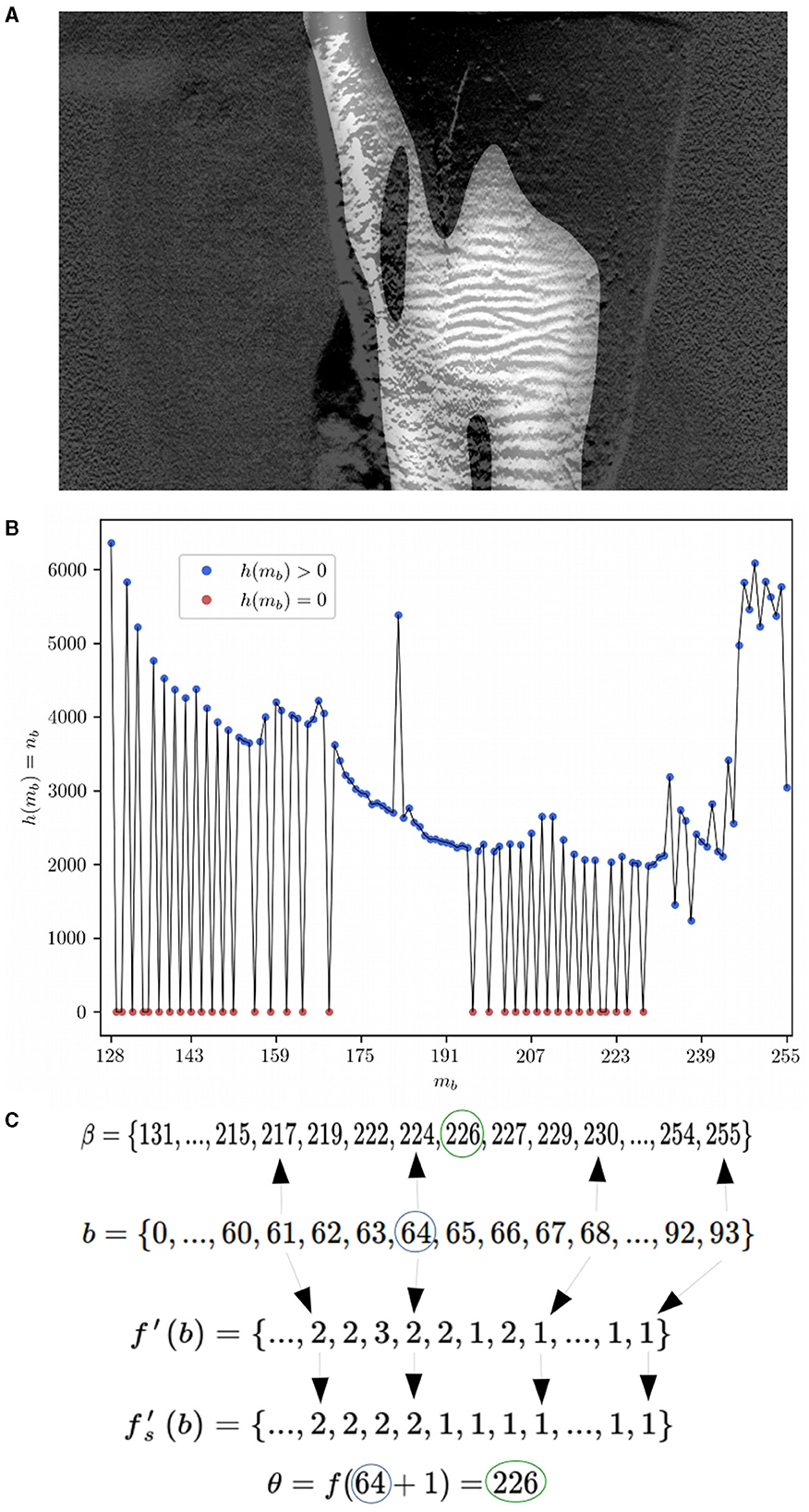
Figure 5. Example of adaptive threshold selection for image 10L2. (A) Heatmap H₃ overlapping image E (resized to J_size for visualization purposes only). Note the higher values of the H₃ heatmap toward the center of the Hunter–Schreger Band region. (B) Histogram of H₃ showing values where m_b > 127, values above zero (blue dots) compose the ordered set β. (C) Illustrated relations between functions and sets to find threshold θ.

We define the function f(.) as

$\begin{array}{ll}f(b)={\beta }_b,& (20)\end{array}$

where β_b is the bth value in β (Figure 5B). We find the adaptive threshold by looking for the last gap greater than one in the sequence of discrete values of β (Figure 5C). For that, the discrete derivative of f(b) is computed as

$\begin{array}{ll}{f}^{\prime }(b)=f(b)-f(b-1).& (21)\end{array}$

To prevent the premature selection of a high threshold and consequently the segmentation of a small region by minor gaps among the β highest values, f′(b) is smoothed by the following linear cross-correlation:

$\begin{array}{ll}{f}_s^{\prime }(b)=\lfloor {\displaystyle \sum _{-\ell }^{\ell }}{W}_{(3)}(\ell )·f^{\prime }(b+\ell )\rfloor ,& (22)\end{array}$

where W₍₃₎ is a linear unit integral kernel of length 3, ℓ = 1, and $f_s^{\prime }(b)\in \mathbb{N}$. To solve the threshold decision, let {1, ..., ȷ} be an ordered set of all b that satisfy the inequality

$\begin{array}{ll}{f}_s^{\prime }(b)>1.& (23)\end{array}$

The final threshold θ to segment H₃ is computed as

$\begin{array}{ll}\theta =f(ȷ+1).& (24)\end{array}$

2.1.7. Obtain raw mask

The raw mask M₁ can be defined as

$\begin{array}{ll}{M}_1(i,j)=\{\begin{array}{l}1if{H}_3(i,j)\ge \theta \\ 0otherwise\end{array}.& (25)\end{array}$

2.1.8. Distance transform

At this point, a segmentation by the M₁ mask might still produce foreground branches that reach outside the ROI. Also, the M₁ mask border might have sharp angles that are not useful for biometric comparisons due to the bands' discontinuity in concave areas. To mitigate this problem, a shrinkage of mask M₁ is performed to remove the branches. Later, a morphological growing is applied to restore its size with a smoother boundary. We first obtain a distance map D using the Euclidean distance transform

$\begin{array}{ll}D(i,j)=min(\{\sqrt{{(i-v)}^2+{(j-u)}^2}\mid (v,u)\in (V,U)\}),& (26)\end{array}$

$\begin{array}{ll}(Y,X)=\left\{(y,x)\mid M_1(i,j)=1\right\},& (27)\end{array}$

$\begin{array}{ll}(V,U)=\left\{(v,u)\mid M_1(v,u)=0\right\},& (28)\end{array}$

where (Y, X) is the set of pairs of the foreground pixel coordinates and (V, U) is the set of pairs of the background pixel coordinates in M₁.

2.1.9. Morphological growing

Afterward, a new background removal is performed on D, with threshold ϕ = max(D)·α, where α determines the reduction rate of D foreground area based on its maximum pixel value. By default, it was set to α = 0.6, resulting in the reduced foreground mask area

$\begin{array}{ll}{M}_r(i,j)=\{\begin{array}{l}1ifD(i,j)>\varphi \\ 0otherwise\end{array}.& (29)\end{array}$

The M_r is repeatedly dilated by a circle-shaped morphological operator ρ_c of radius k_x·0.5 until eventually resulting in the final mask M₂ when any foreground pixel of M_r overlaps with any background pixel in M₁. The pseudocode for this process is described in Algorithm 1.

ALGORITHM 1

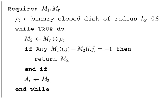
Algorithm 1. Morphological growing mask.

2.1.10. Resize mask and segment image

In the end, the binary mask M₂ is resized back to M×N dimensions, resulting in the M₃ mask, and the final segmented image S_E is defined as

$\begin{array}{ll}{S}_E(i,j)=\{\begin{array}{l}E(i,j)if{M}_3(i,j)>0\\ 0otherwise\end{array}.& (30)\end{array}$

2.2. Fully convolutional neural network

The U-Net was initially created for the precise segmentation of medical images and proved to be useful in diverse branches of medical imaging, including magnetic resonance imaging (MRI; Dolz et al., 2019; Li et al., 2019), optical coherence tomography (OCT; Shah et al., 2018), and microscropy (Cai et al., 2020; Pandey et al., 2020). Due to the high efficiency demonstrated by this neural network when applied in several fields of imaging, we harnessed the architecture of the U-Net to automate the segmentation of the HSBs. The U-Net consists of two parts: an encoder and a decoder. The encoder has four blocks, each one composed of two consecutive convolutions and one max-pooling function. The decoder also has four blocks, each one composed of a deconvolution (up-conv), a concatenation with the intermediate output (copy and stack) from the respective encoder block, followed by two convolutions. The encoder and decoder parts are connected by a “bridge” consisting of two convolutions (Figure 6). Our architecture differs only by image padding, which is the same throughout the network, instead of decreasing; there is no cropping, and the initial image size is a single-channel gray scale of 480 × 320 pixels.

FIGURE 6

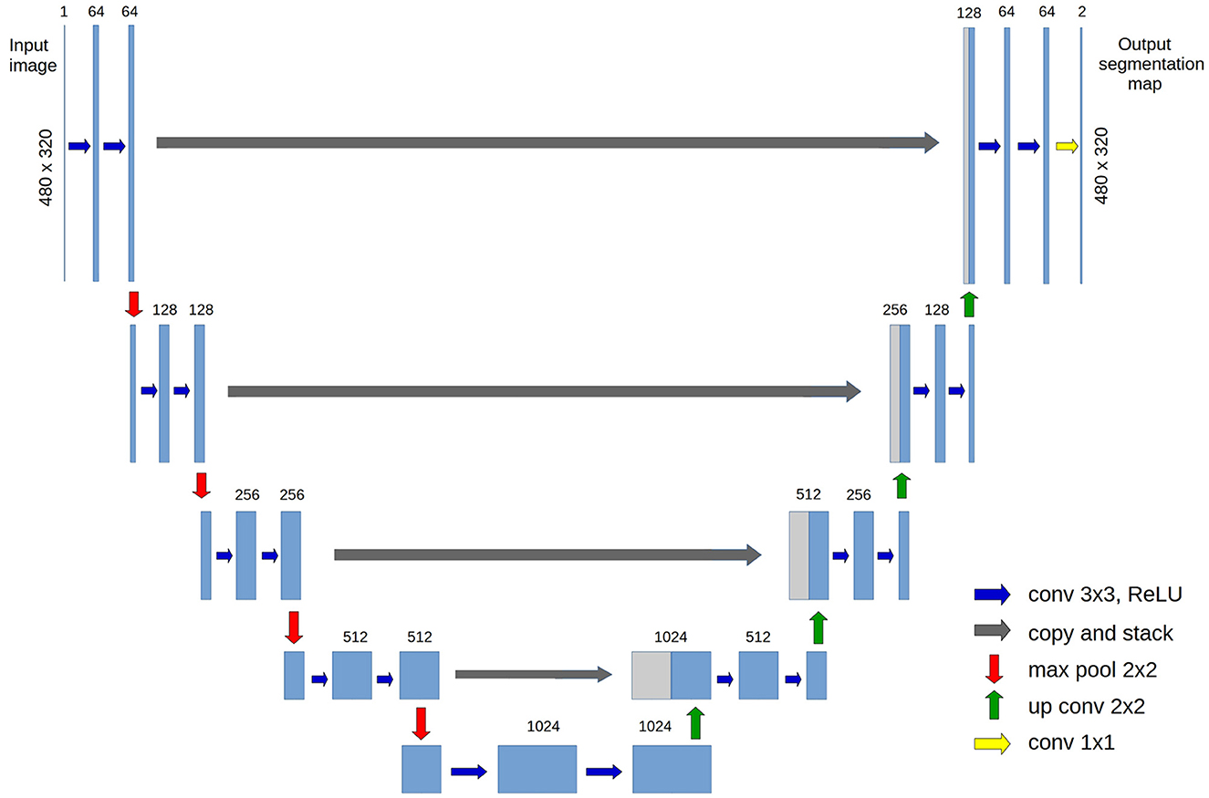
Figure 6. U-Net architecture used; adapted from the original paper (Ronneberger et al., 2015).

The whole data set was divided into three groups: training, validation, and test groups (15, 6, and 10 teeth, that is, 60, 24, and 40 images, respectively). To avoid result bias by the network seeing different images from the same tooth in the training and test groups, we sorted the image such that all four images per tooth went into the same group. The teeth were randomly assigned to each one of the three groups. Regarding the limited data set size for such a deep network, data augmentation during training was performed to maximize variability, creating five variations from each image for training and one variation for the validation group. These augmented images (and their masks) were created randomly over each epoch, being a total of 300 training and 24 validation images per epoch. Since the biometrics protocol in development should accept only images of a tooth positioned vertically, augmentation techniques, for example, rotation, are limited to small ranges in order to be beneficial for the HSB pattern learning. The parameters used for augmentations were rotation {-20, 20} degrees, height, and width shift up to 20%, range in brightness up to 50%, zoom (in or out) up to 20%, and vertical and horizontal flip.

Since the final output image is a binary mask, the final activation is a sigmoid function. The optimizer of choice was Adam, with a learning rate α = 1.0 × 10⁻⁵, and the chosen loss was binary cross-entropy defined as

$\begin{array}{ll}{\text{BCE}}_{loss}=\frac{1}{N}{\displaystyle \sum _{i=1}^N}-\left[(y_{i}ln{p}_i)+(1-y_i)ln(1-p_i)\right],& (31)\end{array}$

where y_i is the true label and p_i is the predicted label for all N pixels in the image. The metric used for assessing performance was Intersection Over Union (IOU). The previously described U-Net was trained over 300 epochs using different batch sizes (1, 5, 10, 15, and 20), and the weights of the epoch with best validation IOU scores were used as the final trained model.

3. Results

In order to assess the results obtained using the developed methods, images were manually segmented to generate a ground truth. The results were assessed by comparing the manual and the automated segmented regions from the same image. The manual selection was performed using the preprocessed grayscale images (Figure 1B) as input images as follows:

1. Selection of region visually greater than HSB area

2. Application of HSB filtering algorithm (“Filtering” in Figure 1) and visual location of improper regions

3. Selection of a smaller and better fitting region if there are improper areas

4. Repetition of steps 2 and 3 until no change is needed

5. Final region is selected.

Since this process gradually decreases the segmented region size, the manually selected ROI is considered to be the largest area with recoverable HSBs, or, more precisely, the largest area whose filtered output image from the HSB filtering algorithm has no visually important deformations for biometric usage.

3.1. ABS experimental results

The previously described ABS algorithm was tested using four sets of images, each from the same 31 extracted teeth. All photographs were taken with the teeth vertically positioned, with the incisal portion upward and cervical portion downward. Two sets were taken with left-side lighting (L1 and L2) and two other sets with right-side lighting (R1 and R2).

The average IOU score between the manual and automated segmented regions overall was 0.766 ± 0.106 SD (standard deviation). The residuals can be separated into an Exclusive Manual-Segmented Regions Over Union (EMSOU), that is, a potential region not selected by the algorithm, and an Exclusive Automate-Segmented Region Over Union (EASOU), which is a trespassed area outside the ROI. Once the EASOU is considered an area with no recoverable HSBs, its minimization is preferred compared to the EMSOU. The average EMSOU was 0.191 ± 0.127 SD and the average EASOU was 0.042 ± 0.044 SD (Table 3 ABS all). The large SD compared to the average for EMSOU and EASOU indicates a non-parametric distribution for these results, with sparse high errors in only a few images, which can be seen in Figure 7. Some examples of ABS performance are shown in Figure 8. In addition to the IOU, the computed FPR (false-positive rate or misclassified background pixels rate) was 0.006, and the FNR (false-negative rate or misclassified foreground pixels rate) was 0.188.

FIGURE 7

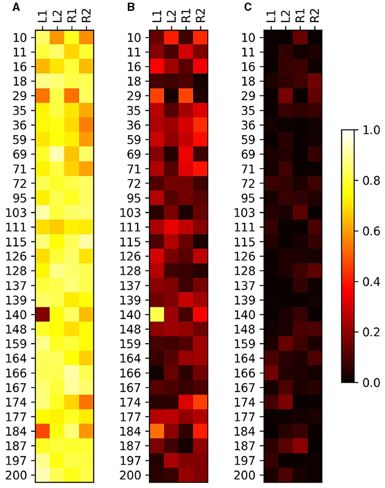
Figure 7. Results of the relation between manual and automated segmentation for the four sets of images of 31 teeth. (A) Intersection Over Union (IOU). (B) Exclusive Manual-Segmentation Region Over Union (EMSOU). (C) Exclusive Automate-Segmented Region Over Union (EASOU). Note that IOU_{i, j}+EMSOU_{i, j}+EASOU_{i, j} = 1, for (i, j)∈ℕ².

FIGURE 8

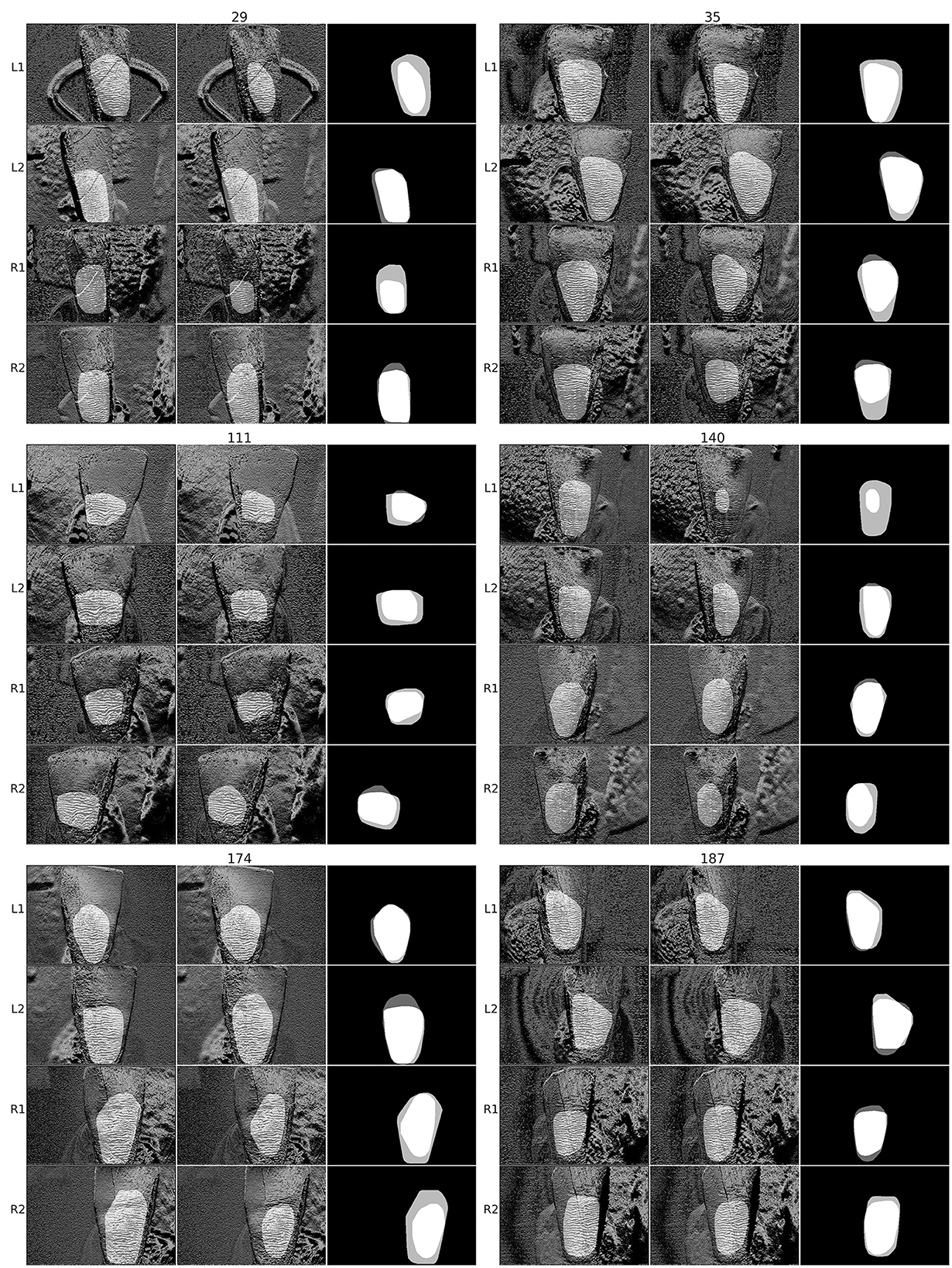
Figure 8. Examples of manual and anisotropy-based segmentation automated segmentation and their mask overlaps for the teeth with indices 29, 35, 111, 140, 174, and 187. The three images for each tooth photograph (L1, L2, R1, R2), from left to right, are HSB image with manual mask, Hunter–Schreger Band (HSB) image with automated mask, and overlap of both masks (white is overlap, light gray is only manual mask, and dark gray is only automated mask).

3.2. U-Net experimental results

According to the training results (Table 1), the hyper-parameter batch size of 5 produced the best result, with a loss of 0.0544 and an IOU score of 0.827 in the validation data set during the training. This IOU score (IOUd) is computed using the predicted decimal values for every pixel in the interval [0, 1] without any thresholding. The training progression loss and IOU score are shown in Figure 9. Other result metrics were very close among all batch sizes.

TABLE 1

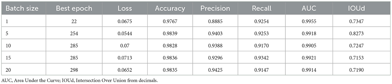
Table 1. Training metrics of the best epoch of validation data set.

FIGURE 9

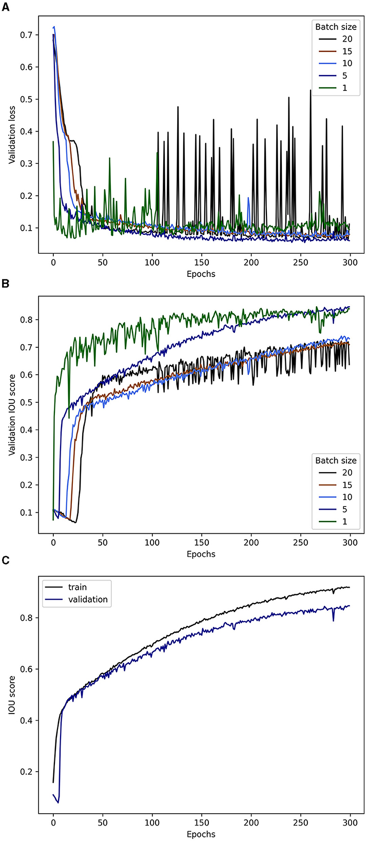
Figure 9. Training progression through epochs. (A) Validation loss. (B) Validation Intersection Over Union (from decimals) score. (C) Training and validation data sets Intersection Over Union in the model with batch size of 5.

The learning curve for batch sizes 5, 10, and 15 was more consistent with increased overfitting (Figure 9), whereas batch sizes of 1 and 20 produced high fluctuation values through the training, with the lowest losses too early and too late, respectively. These cases of high-variability metrics, for example, IOU score, during the training are examples of a trade-off between high-frequency parameter tuning per epoch without generalization by using small batch sizes (the former) and low-frequency parameter tuning per epoch as an attempt for excessive generalizations when using batches that are too large (the latter). It has been shown that large batches tend to reach sharp minima whereas small batches move toward flat minima, reducing the generalization gap (Keskar et al., 2016), that is, the difference between the validation and test data sets results.

3.3. Comparison

The results of evaluation of both models on the test data set are shown in Table 2. The IOU score was computed using the threshold of 0.5 for every pixel with a predicted value in [0, 1]. The model with the best IOU score (0.8393) was the U-Net model trained with a batch size of 15, followed closely by batch sizes of 20, 10, and 5. The least loss (0.0747) was again the model with batch size of 5, with still large differences in the IOUd compared to the other batch sizes (≈0.10). Although a batch size of 15 resulted in better performance on the test data set, the gap between test data set IOUd and IOU scores reveals that all except the batch size of 5 had less confidence in classifying a pixel as foreground or background. This means that the mask output values of the U-Net tend to be closer to the cutoff value for a binary classification, which is usually 0.5 in the range [0,1]. This indicates a high degree of uncertainty and explains the strong variation between the IOUd and IOU scores in these batch size groups. The high uncertainty has been shown to handicap the performance in predicting new data (Dolezal et al., 2022; Yang et al., 2022). The IOU score of the ABS model was the lowest.

TABLE 2

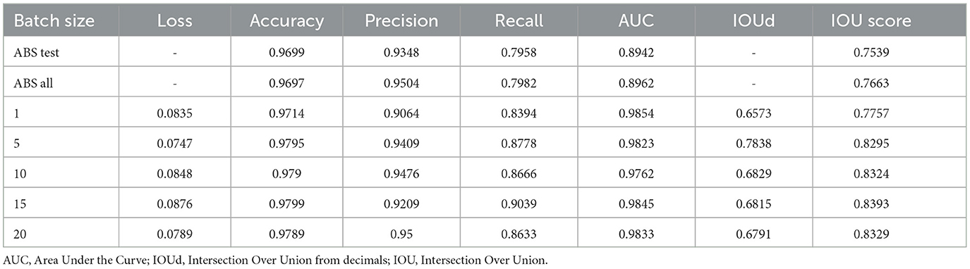
Table 2. Evaluation metrics for U-Net trained models and ABS model for all and only test images.

For further analysis, we kept only the predicted masks by the U-Net model with a batch size of 5 because it has the lowest loss and the lowest gap between the IOUd and IOU scores. The 40 test-predicted masks underwent post-processing by the convex hull algorithm (U-Net-CH; Barber et al., 1996) to also select regions in concave areas left out by the foreground mask. Since the HSB pattern is a radial effect of the light on the enamel subsurface, it usually appears as a convex area. Hence, the concavities of U-Net segmentation might handicap the subsequent biometric performance. The average IOU score between manual and automated segmented regions was 0.837 ± 0.06 SD, that is almost 0.08 above the ABS's. The average EMSOU was 0.101 ± 0.084 SD and the average EASOU was 0.06 ± 0.057 SD. Except for the EASOU score, these results are better than the ones from ABS (Table 3). The U-Net-CH not only improved the IOU and the EMSOU compared to U-Net but also increased average EASOU by 0.009. The U-Net-CH had an FPR of 0.007 and an FNR of 0.122. Compared to the ABS, the FPR of U-Net-CH is slightly higher (about 0.001), meaning its masks more frequently exceed the ROI boundaries, whereas the FNR is significantly lower (about 0.06), meaning it normally selects a larger area inside the ROI. Overall, the trained U-Net-CH was able to select a larger region inside ROI with a slightly greater overpass. The heatmaps for the IOU, EMSOU, and EASOU results are shown in Figure 10 for U-Net-CH and a detailed image-to-image comparison between the models ABS and U-Net-CH is shown in Figure 11 for only the test data set. Some examples of U-Net-CH performance on the test data set can be seen in Figure 12.

TABLE 3

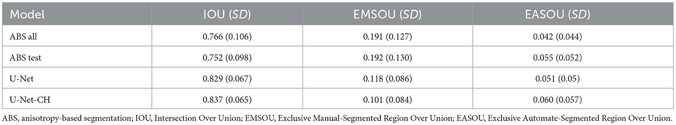
Table 3. Mean and standard deviation of model scores.

FIGURE 10

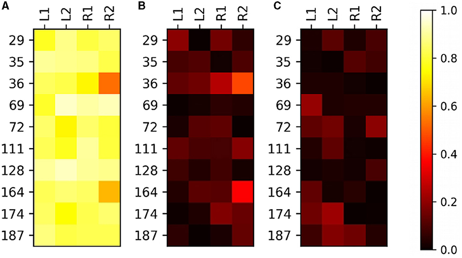
Figure 10. Results of the automated segmentation of U-Net-CH model on test data set. (A) Intersection Over Union (IOU). (B) Exclusive Manual-Segmented Region Over Union (EMSOU). (C) Exclusive Automate-Segmented Region Over Union (EASOU). Note that IOU_{i, j}+EMSOU_{i, j}+EASOU_{i, j} = 1, for (i, j)∈ℕ².

FIGURE 11

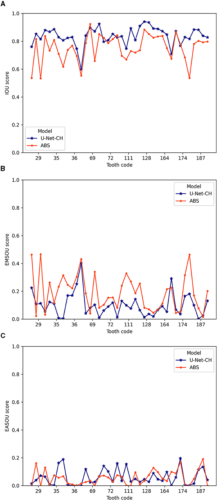
Figure 11. Detailed scores for the 10 teeth (40 images) in the test data set for anisotropy-based segmentation and U-Net-CH. (A) Intersection Over Union (IOU) score. (B) Exclusive Automate-Segmented Region Over Union (EASOU) score. (C) Exclusive Automate-Segmented Region Over Union (EASOU) score.

FIGURE 12

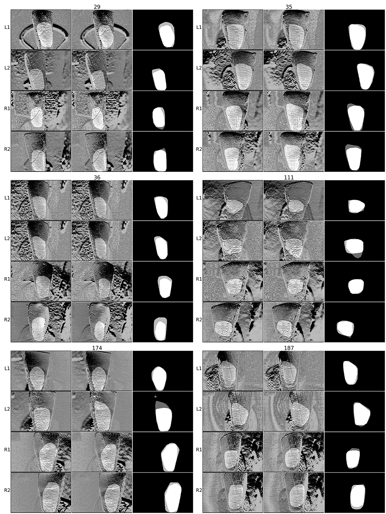
Figure 12. Examples of manual and U-Net-CH automated segmentation and their masks overlap for indexed teeth 29, 35, 36, 111, 174, and 187. The three images for each tooth photograph (L1, L2, R1, R2), from left to right, are Hunter-Schreger Band (HSB) image with manual mask, HSB image with automated mask, overlap of both masks (white is overlap, light gray is only manual mask, and dark gray is only automated mask).

4. Discussion

Currently, both techniques for automated segmentation have acceptable performances regarding ex vivo teeth image sets. While U-Net-CH approach resulted in better segmentation quality, it also had more results overpassing the ground truth boundaries. The ABS is more conservative regarding the boundary limits, resulting not only in smaller segmented regions but also probably in more consistent biometric identification results since fewer false HSBs are selected. Due to the limited sample size for such a deep neural network, that is, the U-Net, increasing the sample size for training the model probably would improve its predictions and might also reduce the most critical error score, that is, the EASOU, of segmented areas. It is worth mentioning that U-Net is extensively used in medical imaging analysis, where biological structures have relatively more precise delimitation, for example, organs in MRI or computed tomography scans, whereas for the proposed application, apart from being convex, the mask is fuzzy and does not fit any particular shape. In addition, different backgrounds should be taken into consideration for training to make sure they will not interfere with the HSB area selection in real applications, where neighboring teeth will likely appear next to the targeted one. Apart from data set specificity, novel variations of U-Net architectures might offer possibilities for further improvement. Examples are the Residual U-Net, based on ResNet (He et al., 2016), which adds skip connections to convolution blocks to prevent the loss of feature identities in deep layers (Siddique et al., 2021; Wang et al., 2021), and the Inception U-Net, which adds an inception module between U-Net convolution block of layers, which consists of filters of different sizes that are concatenated before reaching the next convolution block. The more recent versions of inception architecture have the advantage of reducing the computational cost (Szegedy et al., 2014, 2016; Siddique et al., 2021).

On one hand, the use of ABS might be seamless with limited computational resources and readily available once it is implemented. Moreover, a semiautomated experience can be implemented by offering the user ABS parameters to tweak in order to adapt the algorithm to the nuances the images might have without incurring errors caused by using, for example, a free selection tool. On the other hand, U-Net and its variations trained with a larger data set might achieve more robustness and better overall performance.

5. Conclusion

Automated segmentation is an important step in minimizing human mistakes in image analysis, primarily in the context of repetitive tasks, such as the presented biometric pipeline of HSBs, where multiple teeth should be registered to a database. The acquired performance of both employed methods will ease the development of subsequent processing steps. Apart from the biometric context, further applications of the proposed methods, mainly ABS, may be used to exploit other anisotropic patterns elsewhere.

Data availability statement

The raw data supporting the conclusions of this article will be made available by the authors, without undue reservation.

Ethics statement

The studies involving human participants were reviewed and approved by Research Ethics Committee of the Piracicaba Dental School CAAE 03596918.2.0000.5418. The patients/participants provided their written informed consent to participate in this study.

Author contributions

SL prepared the dental samples and designed the experiment. GF executed the image acquisition, developed the algorithms, and evaluation. SL and DB jointly supervised the project and revised the manuscript. All authors reviewed the manuscript and approved the final manuscript.

Funding

GF was supported by a fellowship from São Paulo Research Foundation (FAPESP, Grants 2018/23038-7 and 2020/07401-4). SL was supported by Grants from FAPESP (2022/10293-4) and Brazilian Council of Scientific and Technological Development (CNPq, 305783/2018-1). In addition, this study was supported by the German Ministry for Education and Research (BMBF) within the Forschungscampus MODAL (Project Grant 3FO18501).

Conflict of interest

The authors declare that the research was conducted in the absence of any commercial or financial relationships that could be construed as a potential conflict of interest.

Publisher's note

All claims expressed in this article are solely those of the authors and do not necessarily represent those of their affiliated organizations, or those of the publisher, the editors and the reviewers. Any product that may be evaluated in this article, or claim that may be made by its manufacturer, is not guaranteed or endorsed by the publisher.

References

Arrieta, Z. L., Fogalli, G. B., and Line, S. R. P. (2018). Digital enhancement of dental enamel microstructure images from intact teeth. Microsc. Res. Tech. 81, 1036–1041. doi: 10.1002/jemt.23070

PubMed Abstract | CrossRef Full Text | Google Scholar

Arrieta, Z. L., and Line, S. R. P. (2017). Optimizing the analysis of dental enamel microstructure in intact teeth. Microsc. Res. Tech. 80, 693–696. doi: 10.1002/jemt.22852

PubMed Abstract | CrossRef Full Text | Google Scholar

Barber, C. B., Dobkin, D. P., and Huhdanpaa, H. (1996). The quickhull algorithm for convex hulls. ACM Trans. Math. Softw. 22, 469–483.

PubMed Abstract | Google Scholar

Cai, S., Tian, Y., Lui, H., Zeng, H., Wu, Y., and Chen, G. (2020). Dense-UNet: a novel multiphoton in vivo cellular image segmentation model based on a convolutional neural network. Quant. Imaging Med. Surg. 10, 1275–1285. doi: 10.21037/qims-19-1090

PubMed Abstract | CrossRef Full Text | Google Scholar

Dolezal, J. M., Srisuwananukorn, A., Karpeyev, D., Ramesh, S., Kochanny, S., Cody, B., et al. (2022). Uncertainty-informed deep learning models enable high-confidence predictions for digital histopathology. Nat. Commun. 13, 6572. doi: 10.1038/s41467-022-34025-x

PubMed Abstract | CrossRef Full Text | Google Scholar

Dolz, J., Desrosiers, C., and Ben Ayed, I. (2019). “IVD-Net: intervertebral disc localization and segmentation in MRI with a multi-modal UNet,” in Computational Methods and Clinical Applications for Spine Imaging, eds G. Zheng, D. Belavy, Y. Cai, and S. Li (Cham: Springer International Publishing), 130–143.

Google Scholar

Fogalli, G. B., Line, S. R. P., and Baum, D. (2022). “Automatic segmentation of tooth images: optimization of multi-parameter image processing workflow,” in EuroVis 2022 - Posters, eds M. Krone, S. Lenti, and J. Schmidt (Eindhoven: The Eurographics Association), 11–13.

Google Scholar

He, K., Zhang, X., Ren, S., and Sun, J. (2016). “Deep residual learning for image recognition,” in 2016 IEEE Conference on Computer Vision and Pattern Recognition (CVPR), 770–778.

PubMed Abstract | Google Scholar

Keskar, N. S., Mudigere, D., Nocedal, J., Smelyanskiy, M., and Tang, P. T. P. (2016). On large-batch training for deep learning: generalization gap and sharp minima. arXiv preprint arXiv:1609.04836.

Google Scholar

Koenigswald, W. v. (1994). U-shaped orientation of hunter-schreger bands in the enamel of moropus (mammalia: Chalicotheriidae) in comparison to some other perissodactyla. Ann. Carn. Museum 63, 49–65.

Google Scholar

Li, S., Chen, Y., Yang, S., and Luo, W. (2019). “Cascade dense-unet for prostate segmentation in MR images,” in Intelligent Computing Theories and Application, eds D.-S. Huang, V. Bevilacqua, and P. Premaratne (Cham: Springer International Publishing), 481–490.

Google Scholar

Line, S. R. P., and Bergqvist, L. P. (2005). Enamel structure of paleocene mammals of the São José de Itaboraí Basin, Brazil. ‘Condylarthra', Litopterna, Notoungulata, Xenungulata, and Astrapotheria. J. Verteb. Paleontol. 25, 924–928. doi: 10.1671/0272-4634(2005)0250924:ESOPMO2.0.CO;2

CrossRef Full Text | Google Scholar

Pandey, R., Lalchhanhima, R., and Singh, K. R. (2020). “Nuclei cell semantic segmentation using deep learning UNet,” in 2020 Advanced Communication Technologies and Signal Processing (ACTS) (IEEE), 1–6.

Google Scholar

Ramenzoni, L. L., and Line, S. R. (2006). Automated biometrics-based personal identification of the hunter–schreger bands of dental enamel. Proc. R. Soc. B Biol. Sci. 273, 1155–1158. doi: 10.1098/rspb.2005.3409

PubMed Abstract | CrossRef Full Text | Google Scholar

Ronneberger, O., Fischer, P., and Brox, T. (2015). “U-Net: convolutional networks for biomedical image segmentation,” in International Conference on Medical Image Computing and Computer-Assisted Intervention (Cham: Springer International Publishing), 234–241.

Google Scholar

Shah, A., Zhou, L., Abrámoff, M. D., and Wu, X. (2018). Multiple surface segmentation using convolution neural nets: application to retinal layer segmentation in OCT images. Biomed. Opt. Express 9, 4509. doi: 10.1364/BOE.9.004509

PubMed Abstract | CrossRef Full Text | Google Scholar

Shen, W., and Tan, T. (1999). Automated biometrics-based personal identification. Proc. Natl. Acad. Sci. U.S.A. 96, 11065–11066.

Google Scholar

Siddique, N., Paheding, S., Elkin, C. P., and Devabhaktuni, V. (2021). U-net and its variants for medical image segmentation: a review of theory and applications. IEEE Access 9, 82031–82057. doi: 10.1109/ACCESS.2021.3086020

CrossRef Full Text | Google Scholar

Sweet, D., and Sweet, C. (1995). DNA analysis of dental pulp to link incinerated remains of homicide victim to crime scene. J. Forens. Sci. 40, 310–314.

PubMed Abstract | Google Scholar

Szegedy, C., Vanhoucke, V., Ioffe, S., Shlens, J., and Wojna, Z. (2016). “Rethinking the inception architecture for computer vision,” in 2016 IEEE Conference on Computer Vision and Pattern Recognition (CVPR) (Los Alamitos, CA: IEEE Computer Society), 2818–2826.

Google Scholar

Szegedy, C., Liu, W., Jia, Y., Sermanet, P., Reed, S., Anguelov, D., Erhan, D., et al. (2014). Going deeper with convolutions. arXiv preprint arXiv:1409.4842. doi: 10.1109/CVPR.2015.7298594

CrossRef Full Text | Google Scholar

Tseng, Z. J. (2012). Connecting hunter-schreger band microstructure to enamel microwear features: new insights from durophagous carnivores. Acta Palaeontol. Polonica 57, 473–484. doi: 10.4202/app.2011.0027

CrossRef Full Text | Google Scholar

Valenzuela, A., de las Heras, S. M., Marques, T., Exposito, N., and Bohoyo, J. M. (2000). The application of dental methods of identification to human burn victims in a mass disaster. Int. J. Legal Med. 113, 236–239. doi: 10.1007/s004149900099

PubMed Abstract | CrossRef Full Text | Google Scholar

von Koenigswald, W., Rensberger, J. M., and Pretzschner, H. U. (1987). Changes in the tooth enamel of early paleocene mammals allowing increased diet diversity. Nature 328, 150–152.

PubMed Abstract | Google Scholar

Wang, Z., Zou, Y., and Liu, P. X. (2021). Hybrid dilation and attention residual U-Net for medical image segmentation. Comput. Biol. Med. 134, 104449. doi: 10.1016/j.compbiomed.2021.104449

PubMed Abstract | CrossRef Full Text | Google Scholar

Whittaker, D., and Rothwell, T. (1984). Phosphoglucomutase isoenzymes in human teeth. Forens. Sci. Int. 24, 219–223.

Google Scholar

Yang, Z., Lafata, K., Vaios, E., Hu, Z., Mullikin, T., Yin, F.-F., et al. (2022). Quantifying U-Net uncertainty in multi-parametric MRI-based glioma segmentation by spherical image projection. arXiv preprint arXiv:2210.06512.

Google Scholar