A Novel Machine-Learning Framework With a Moving Platform for Maritime Drift Calculations

1 Introduction

1.1 Overview

Predicting the drift of objects in the ocean is an important and complex scientific problem. The trajectory of a drifting object on the sea surface is the net result of the aerodynamic and hydrodynamic forces acting on it. The direction of the drift is not always toward the wind, and its direction relative to the wind direction is referred to as the drift or divergence angle. The drift velocity can be resolved as a component in the direction of the leeway, referred to as the downwind drift leeway component (DWL), and the perpendicular component is the crosswind drift leeway component (CWL). Due to the unsteady nature of the wind and oceanic forces, estimating the forces in real time is extremely challenging. While the laws of physics for predicting the leeway trajectory of objects in open surfaces are well understood, the accuracy of the prediction of the leeway trajectory can be affected by the uncertainty of uncontrollable factors. The fundamental challenges in making forecasts in search areas are the errors that may arise due to the uncertainties that come from (a) the measurements of unsteady ocean current forcings, wind fields, turbulence mixing, and wave effects Breivik and Allen (2008); (b) the poor estimates of the real drift properties of the drifting object; and (c) the estimation of the drag forces acting on the drifting object. The unsteadiness and variation of the drag forces further complicate the problem. As the drift depends on the percentage of immersion of the object in the water, using a shape-dependent coefficient is not sufficient. The percentage of immersion should be accounted for in the model to be used. However, this information cannot be obtained a priori, which makes the model calculations uncertain.

An alternative method of calculating the leeway drift in real time is the focus of the present work. With the recent advances in machine learning and sensing technology; detecting and tracking a drifting object can be achieved with a high degree of precision. However, as the object is moving, its detection and tracking are prone to errors, and hence, combining machine learning and sensing technology with deep-learning models, which are mostly data driven, will make them robust to different types of uncertainty. An additional challenge with the objects drifting in the ocean is that the search area is very large, making it impossible to use a stationary sensing platform to detect them. Thus, we developed a technology specifically for a moving platform. The platform is to be deployed on a manned boat that can actively detect, track, and follow a drifting object in real time.

1.2 Background

Maritime search and rescue (SAR) is one of the United States Coast Guard’s (USCG) oldest missions. USCG maintains a high state of vigilance and readiness, engages in continuous distress monitoring, and employs sophisticated drift modeling and search optimization tools to improve its SAR planning and execution. In 2020, USCG responded to a total of 16,845 SAR cases, assisted 21,050 people, and saved 4,286 lives in imminent danger Buchman (2020).

Several operational forecast models for predicting the evolution of search areas for drifting objects have appeared of late Allen and Plourde (1999); Hackett et al. (2006); Donnell et al. (2006); Breivik and Allen (2008); Davidson et al. (2009). These models rely on Monte Carlo (stochastic) techniques to compute the coordinates of probable search areas from ensemble trajectory models that take into account the near-surface currents, the wind field, and the object-specific drift properties that may advect the drifting object. Simple linear regression coefficients have been proven to be the preferred tools for obtaining the parameters of the leeway of distressed objects in the SAR community Breivik and Allen (2008), but conducting field experiments to determine the drift properties of objects for the development of a database for drifting objects is costly Allen and Plourde (1999). Nonetheless, without a proper estimate of the basic drift properties and their associated uncertainties, forecasting the drift and expansion of a search area will remain difficult. With the recent advances in numerical modeling, high-resolution meteorological and ocean models are now capable of generating near-surface wind fields and surface currents. The fact that most leeway cases occur near the shoreline and in partially sheltered waters Breivik and Allen (2008) further compounds the difficulties involved as the resolution of operational ocean models in many places of the world is still insufficient to determine the nearshore features. The diffusivity of the ocean is an important factor when reconstructing the dispersion of particles on the basis of either the observed or modeled vector fields. Regional and possibly seasonal estimates of diffusivity and the integral time scale significantly affect the dispersion of drifting objects.

1.3 Perception Sensing

Maritime SAR operation needs a fast paced planning and execution speed but performing this search operation comes with its own issues. The search must be quick to shorten the detection time. In terms of perception, the object of interest may have a different level of immersion, lighting condition (due to weather or time of day), or obstruction between maritime boat and object of interest. In addition, precise scanning of objects is required to determine if the detected object is the target object. These requirements have a trade-off relationship because an increase in search speed inevitably decreases the precision with which the object is identified.

A promising solution to this problem is based on the use of multiple sensing techniques Wang et al., 2007; Shafer et al. (1986); Hackett and Shah (1990). LiDARs provide sparse panoramic information on the environment and have become increasingly popular Cesic et al. (2014). Capable of providing panoramic measurements up to 100 meters and at a reasonable rate of 10–15Hz. Thus making it the ideal option for objection detection and tracking of moving objects in the marine environment. However, they have a major disadvantage; they do not have the resolution needed to identify the shape of the drifting object.

The aforementioned problem can be resolved by utilizing depth perception cameras (also known as stereo cameras). Stereo cameras are capable of capturing data-rich images along with their depth information. These high-dimensional data (both image and depth information) needs to be processed with advanced algorithms that require high computing power. Even then, the data collected will be affected directly due to inadequate lighting, visibility, and weather conditions. Despite their limitations, computer vision algorithms have been developed to efficiently perform tasks like object detection Breitenstein et al. (2010); Kyto et al. (2011); Biswas and Veloso (2012); Redmon et al. (2016a). These methods are much cheaper than LiDARs Hall and Llinas (1997). Hence, the SAR community prefers them to other sensors for detecting moving objects. Both LiDARs and depth cameras contain depth sensors, but while depth cameras obtain depth information using the disparity information in the image, LiDARs obtain depth information from the environment. Each sensor has its pros, and cons Hall and Llinas (1997); Hall and McMullen (2004). Depth cameras provide rich depth information, but their field of view is quite narrow. Conversely, LiDARs contain a wider field of view, but they provide sparse rather than rich environment information Akhtar et al. (2019). LiDARs provide information in the form of a point cloud, whereas depth cameras provide luminance. It is evident that these sensors can complement each other and can be used in tandem in complex applications [Steinberg and Bowman (2007); Crowley and Demazeau (1993)]. In this work, we developed a hardware framework to align and fuse the data collected from IMU sensors, GPS data, stereo cameras, and LiDARs for monitoring a large area of interest. Later, we propose an integrated machine learning framework to identify, track, and estimate an object’s drifting trajectory in the wild in real-time using the collected data.

1.4 Machine Learning Framework for Detection and Tracking

A significant level of progress has been made in the field of object detection and tracking due to the development of deep learning LeCun et al. (2015). Additionally, continuous improvement of computing power has made it further possible to train and deploy these models for day to day use.

Object detection tasks can be divided into two major topics (1) Generic object detection: for the objects that are present around us in day to day application, and (2) application specific object detection: for objects in specific domains and use cases such as human in a marine search and rescue scenario Zou et al. (2019). Object detection has become popular due to its capability of using versatile real-world applications such as autonomous driving, robot vision, manufacturing defect detection, and maritime surveillance. All this was possible due to the development AlexNet Krizhevsky et al. (2012) which started the deep learning revolution in generic object detection followed by the development of other deep learning methods for object detection Girshick et al. (2014); Ren et al. (2016); Mask (2017); Liu et al. (2020). For a detailed list of development in this field, we encourage the reader to read the work by Li et al. Liu et al. (2020) and Jiao et al. (2019). In this work we propose to use a one-stage object detector proposed by Redmond et al. known as YOLO (You Only Look Once) Redmon and Farhadi (2017); Redmon et al. (2016b). YOLO is one of the extremely fast object detection algorithms that achieves 155fps (faster version)and 45fps (enhanced version) in edge devices (and webcam’s). YOLO defines the detection problem as a regression problem, so an unified architecture can extract features from input images straightly to predict bounding boxes and class probabilities directly. We implemented the version 3 of YOLO which can detect small scale to large scale objects in images which is a good fit for our case considering SAR’s parameters.

SAR operations require a quick detection and tracking time. However, performing detection at each frame is a computationally expensive task and increases the detection and tracking time. Thus to speed up the process, instead of running the detection algorithm at each frame, we detect an object at one frame and keep track of the object in consecutive frames utilizing a tracking algorithm. After a certain number of frame, we rerun the detection algorithm to detect objects in the frameLukezic et al. (2017); Behrendt et al. (2017). Furthermore, we utilize the stereo images collected from the cameras to train a second deep learning model to estimate the depth (or distance) of the objects with respect to the base location Chang and Chen (2018). The estimated depth is further processed to calculate the trajectory of the object of interest. Below are the objectives of the study-

1. To design and construct an observational data collection platform consisting of stereoscopic depth cameras, a rotating LiDAR, a global positioning system (GPS), an inertial measurement unit (IMU), a wind anemometer, an ocean current profiler, and an on-board computing unit to be mounted on a moving surface vehicle.

2. To develop a machine learning algorithm for detecting and tracking drifting objects in real time.

3. To calculate the leeway drift coefficients of pelicans, a floating person in water (PIW), and a partially submerged PIW.

The rest of this paper is organized as follows: Section 2 discusses the hardware technology used in the study and the developed machine learning framework. Section 2.1 discusses the hardware data collection platform, section 2.2 describes the object detection and tracking methods using machine learning algorithms, Section 2.3 discusses the details of the field tests. The results are presented in section 3, and section 4 presents the study conclusions.

2 Framework and Methodology

The framework for the hardware architecture that was used in the present study and for the method of detecting and tracking the target object using machine learning is described in this section. We first describe the hardware consisting of the operational platform, which had perception-based sensors, a GPS, an IMU, and a computer, followed by the environmental sensors consisting of a wind anemometer and an ocean current buoy. We then describe the moving platform and discuss how the sensors record the data with respect to such platform and how the frame of reference is transformed into a fixed one from a moving one. Finally, the test data and conditions are described.

2.1 Hardware: Data Collection Observational Platform

The hardware that was used in the present study consisted of a data collection platform, a detachable module that could be mounted on any surface vehicle, as shown in Figure 1. It consisted of a LiDAR sensor, stereoscopic depth cameras, a Piksi GPS, an IMU, and a computer. The details of each of these components are provided in the following sections. The data obtained from all the perception-based sensors and those obtained from the on-board meteorological tower and the ocean current profiler deployed in the ocean were collected and processed by the onboard computer. The perception-based sensors were the Ouster OS2-128 and MultiSense S21B stereo cameras. The setup consisted of a front-facing camera (facing the bow of the boat), a real-facing camera (facing the stern of the boat), and two cameras with a 180° distance between them and with an approximately 10° focal-view overlap. The LiDAR sensor was placed on an elevated mount at the center of the boat.

FIGURE 1

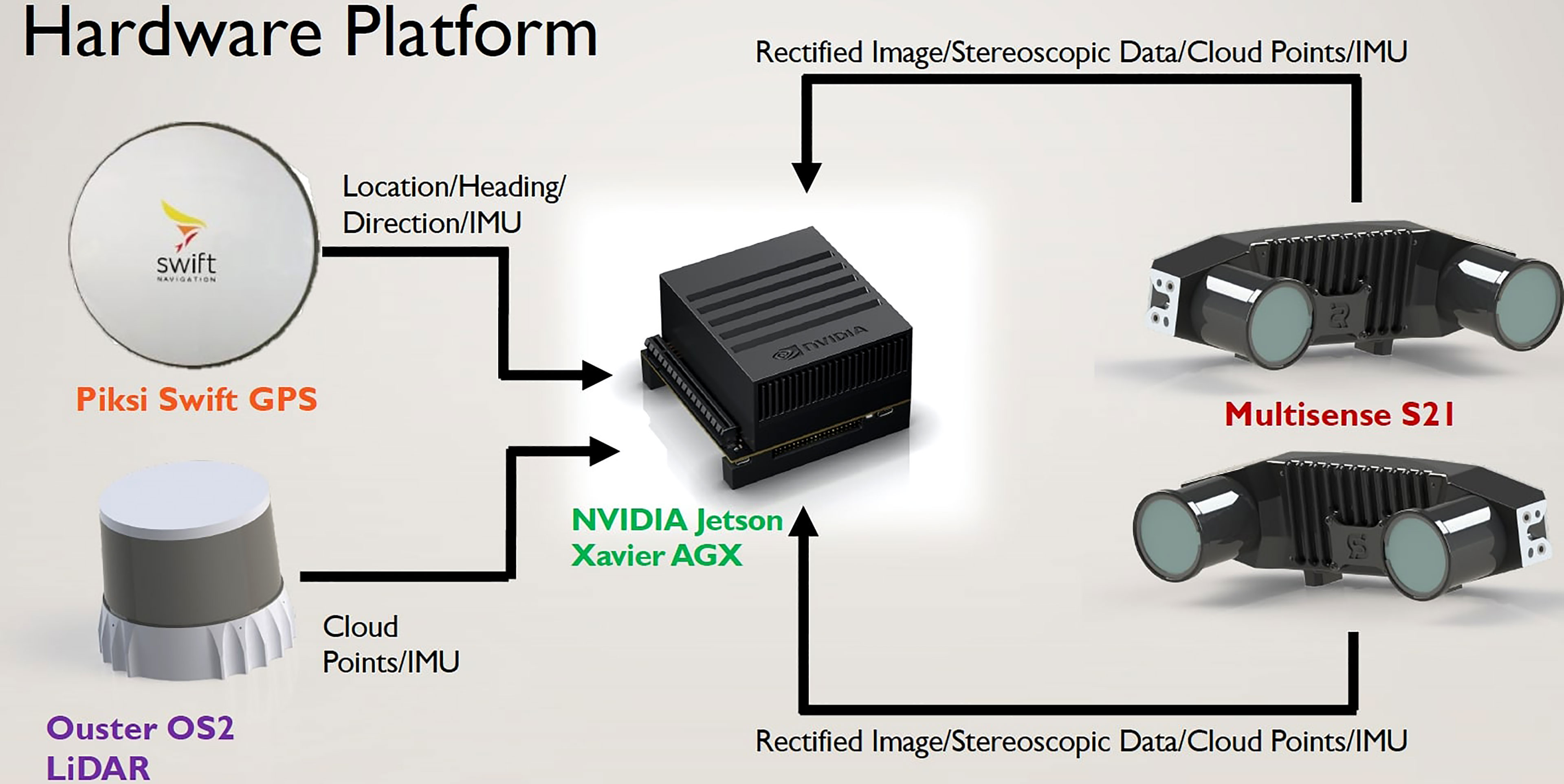
Figure 1 Flow chart showing the sensors connected to the computing unit.

The modules of the hardware platform from Figure 1 are explained here:

2.1.1 Light Detector and Ranging

LiDAR is a remote sensing technology that illuminates an area with a light source in the form of a pulsed laser. The light pulses are scattered by the objects in the scene and are detected by a photo detector. LiDAR sensors are currently the primary sensors used due to their detection accuracy, higher data resolution than other sensors, and capability of determining the shapes of objects. LiDAR sensors can provide precise three-dimensional (3D) information on the shape of an object and its distance from the source by measuring the time it takes for the light to travel to the object and back. LiDAR sensors are thus very useful in detecting objects and developing an environment model. However, they have both advantages and disadvantages. Their advantages include usage safety, fast scans of the environment, and high accuracy. Some LiDAR sensors can capture data even at a 2,500 m distance and have better resolution than other scan systems, like radars. As for their disadvantages, they are very expensive, the data that they provide are not as rich as those provided by an RGB (red, green, and blue) camera with a good resolution, a single data point may not be accurate, and high-volume data points may need to be used, their scans and eventual point clouds are too big and consume much space. Two-dimensional LiDAR sensors are mainly useful as line scanners and are sparingly used.

2.1.2 Stereoscopic Depth Camera

Stereo vision sensors provide depth information. The benefits of using this combined with a LiDAR sensor are the accuracy, speed, and resolution of the LiDAR sensor and the quality and richness of the data from the stereo vision camera. Together, the LiDAR sensor and the stereo vision camera provide an accurate, rich, and fast dataset for the object detection layer. For the precise tracking of a moving object in real time, accurate data from each of the sensors are required. An RGB (red, green, blue) camera is equipped with a standard CMOS (complementary metal-oxide-semiconductor) sensor through which the colored images of the world are acquired. The advantages of RGB cameras are their wide availability, affordability, and ease of use, not needing any specialized driver. As for their disadvantages, they require good lighting, the high-end ones with an excellent resolution are costly, and some of them cannot efficiently capture reflective, absorptive, and transparent surfaces such as glass and plastic. For the present study, we used a 360° camera, which captures the dual images and video files from dual lenses with a 180° field of view and either performs automatic on-camera stitching of the images/videos or allows the user to perform off-board stitching of the images/videos to provide a 360° view of the world; Guy; Sigel et al. (2003); De Silva et al. (2018a, 2018b).

2.1.3 Localization Module

The localization module informs the boat of its current position at any given time. A process of establishing the spatial relationship between the boat and stationary objects’ localization is achieved using devices like GPS, odometer sensors, and IMU. These sensors provide the position information of the sensing system, which can be used by the system to see where it is situated in the environment.

2.1.4 Sensor Data Alignment: Transformation

Locating leeway objects is an interesting problem as the objects need to be located in highly nonlinear, dynamic environments. If the environment does not change, the detection is usually straightforward. In this case, however, due to the dynamic nature of the environment and the objects of interest, the problem becomes complex. Keeping this scenario in mind, we used a tiered approach to detecting leeway objects. We first used LiDAR scans because the sensor can scan objects upwards of 200 m from the sensor whereas cameras can locate objects only 40–50 m from the sensor. The system first tries locating the object through a LiDAR scan and then tries to locate the object when it is closer using the integrated information from the camera and the LiDAR sensor. The data collected from the sensors are according to their respective frames of reference. The data obtained from all the sensors should then be converted into a uniform reference frame. One of the ways to do this is by using transforms between the three sensors. To detect a leeway object using the two stereo cameras and the LiDAR sensor, we determined the transforms between them and a base point. We used the base of the sensor mount as the base point. First, we calculated the transforms of the sensor base to the LiDAR sensor, which provided the position of the LiDAR sensor with respect to the sensor base. We then calculated the transforms of the two MultiSense S21B cameras; this provided the positions of the two cameras relative to each other. We then determined the transforms between the LiDAR sensor and the two cameras. After completing this step, we obtained a full-transform tree of the three sensors. After the successful data integration, we used the information that we obtained to locate the target moving objects.

2.1.5 Environmental Sensors

The gill wind anemometer is used to measure the wind speed and direction. For the data collection in the present study, a 2007 VIP Model 2460 boat from USCG was used. The boat was 25 ft long and had four poles connecting the roof to the ground. Using the poles placed in the port-stern side of the boat (left-rear), we attached the sensor base to the round central mount sign bracket and then to the pole on the boat. The gill wind sensor was mounted relative north. The sensor is located at a height of 3 ft above the surface of the boat. The reference was directed to the front of the boat. The GPS mounted on the boat was used to calculate the wind speed and direction with respect to the geographical north.

The ocean currents were measured using an Eco acoustic Doppler current profiler (ADCP) designed for shallow-water measurements. It measures water velocities in-situ, through the water column using the acoustic Doppler technology. A buoy is used deploy the current profiler into the waters.

2.2 Machine Learning Framework

The machine learning framework consists of three distinct modules. The modules being: (1) Detection Module, (2) Tracking Module, and (3) Distance Mapping Module. The first two module works in a synergy to speed up the detection and tracking process, while the third module maps the distance of the detected/tracked object utilizing the stereo camera images. Below we describe each module separately-

2.2.1 Object Detection Framework

The aim of the object detection module is to identify the desired features within a region of interest. For example, a trained object detector aims to identify all the humans present in a given image frame. At stage one, it looks into parts of the image that have a high probability of containing the target object. Once the features of interest are identified, the module labels them (or counts the number of objects present). The algorithm that is used is the YOLOV3 model. YOLO is orders of magnitude faster (45 frames/s) than other object detection algorithms (e.g., MobileNetV3, YOLOV2) and was designed with mobile devices in mind to support classification, detection, and tracking. Figure 2 shows the combined operation steps for detection and Tracking for our combined step.

FIGURE 2

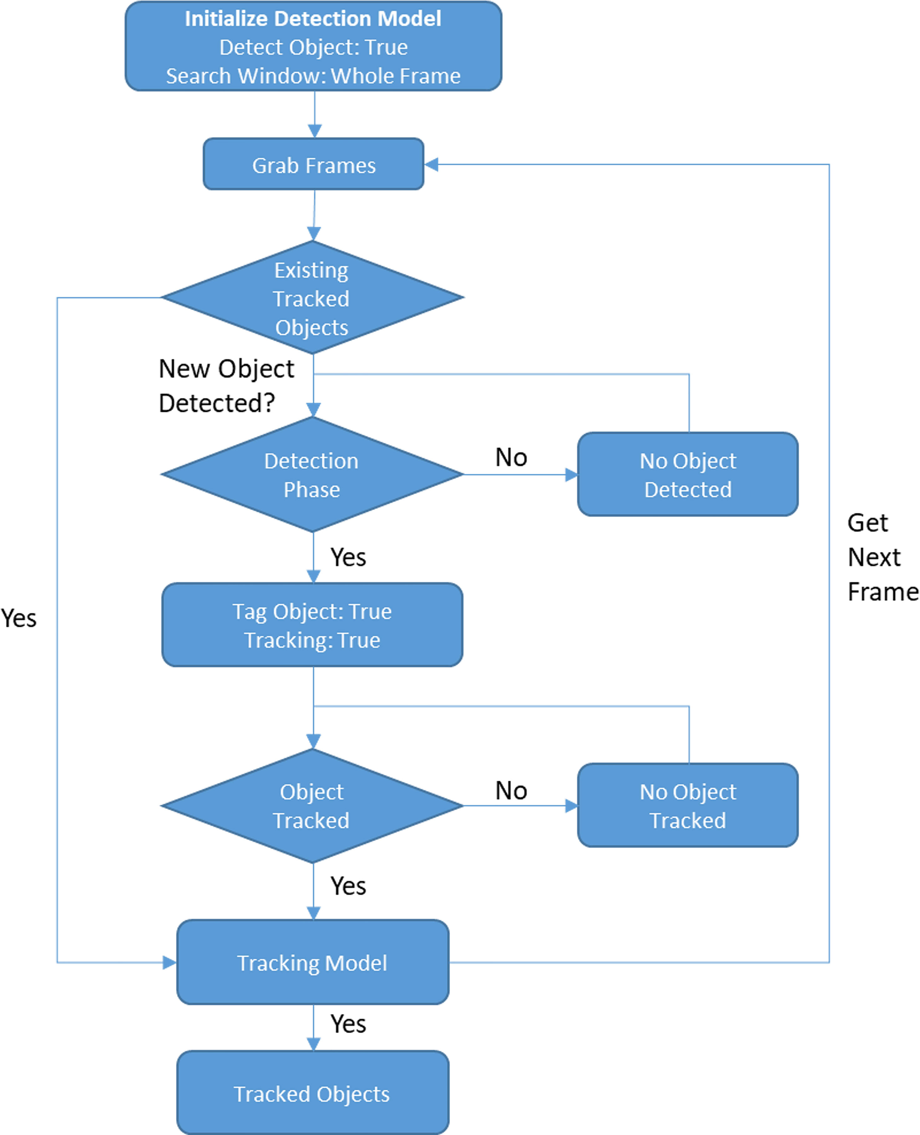
Figure 2 Overall steps for detection and tracking.

YOLO is a unified detector that poses object detection as a regression problem. The network divides the images into several regions and approximates the bounding boxes for detected objects and probabilities for each of the regions simultaneously. Let X represents an image, the pipeline divides the image into m × m grids. Each grid cell is tested to determine the presence of each predicting class probabilities C, bounding box, B, and their confidence score. As YOLO scans the whole image X while making a prediction, it implicitly encodes contextual information about object classes, its less likely to predict false-positive classes and bounding boxes Redmon and Farhadi (2017); Redmon et al. (2016a). YOLOV3 has 53 convolution layers called Darknet-53. It uses utilizes the sum of squared errors (SSE)/loss function to optimize their network. However, Redmon et al. (2016a, 2016b); modified the loss function to reflect their objective of maximizing the average precision. They increased the loss coming from bounding box coordinate prediction and decreased the loss from confidence predictions for boxes that contain detected objects. Thus, the loss functions becomes-

$\begin{array}{ll}\begin{array}{c}ℒ={\lambda }_{coord}{\displaystyle \sum _{i=0}^{S^2}}{\displaystyle \sum _{\underset{+}{j=0}}^B}{1}_{ij}^{obj}[{(x_i-{\widehat{x}}_i)}^2+\hspace{0.17em}{(y_i-{\widehat{y}}_i)}^2]+{\lambda }_{coord}{\displaystyle \sum _{i=0}^{S^2}}{\displaystyle \sum _{j=0}^B}{1}_{ij}^{obj}[{(\sqrt{w_i}-\sqrt{{\widehat{w}}_i})}^2+{(\sqrt{h_i}-\sqrt{{\widehat{h}}_i})}^2]\\ {\displaystyle \sum _{S^2}^{S^2}{\displaystyle \sum _{j=0}^B{1}_{ij}^{obj}[{(C_i-{\widehat{C}}_i)}^2+{\lambda }_{noobj}}{\displaystyle \sum }_{i=0}^{S^2}{\displaystyle \sum }_{j=0}^B{1}_{ij}^{noobj}[{(C_i-{\widehat{C}}_i)}^2}\\ {\displaystyle \sum _{i=0}^{S^2}{1}_{ij}^{obj}{\displaystyle \sum _{c\in classes}{\left(p_i\left(c\right)-{\widehat{p}}_i\left(c\right)\right)}^2}}\end{array}& (1)\end{array}$

where, $1_{ij}^{obj}$ denotes if an object appears in i^th cell and if j^th bounding box in i^th cell is “responsible” for the prediction. The loss function only penalizes the classification error if an object is present in a grid cell. The first two terms represent the localization loss. The first term calculates the SSE between the predicted bounding box and ground truth coordinates, and the second term calculates the SSE in the bounding box dimensions. Here, $1_{ij}^{obj}=1$ the box contains an object and is responsible for detecting this object (higher IOU) else. $\widehat{C}=1$ The third term is confidence error where $\widehat{C}=1$ and 0 ≤ C ≤ 1. If there is no object in the grid the localization and classification error is ignored and confidence error is calculated. Here,

$1_{ij}^{noobj}=1$ if there is no object in the grid else 0. Since most grids will not contain any object, this term pushes the confidence scores of those cells towards zero which is the value of the ground truth confidence. To avoid the divergence due to the large number of these types of grids we assign λ_noobj =0.5 The last term calculates the class probabilities.

We utilized mean average precision (mAP) to evaluate the performance of the detection module. This is also referred to as average precision (AP) and is a popular metric used to measure the performance of models doing document/information retrieval and object detection tasks. mAP is defined as -

$\begin{array}{ll}mAP={\displaystyle \sum _{q=1}^Q\frac{AveP\left(q\right)}{Q}}& (2)\end{array}$

Where, Q is the number of queries in the set and AveP(q) is the average precision (AP) for a given query q.

2.2.2 Object Tracking Framework

This module follows/determines the location of the features identified in the detection phase through consecutive images. Detection is generally computationally expensive, but utilizing a tracking module allows computation after the analysis of the first frame of an image. For example, when an object of interest (say a pelican) is identified at the first frame of the video stream, from the next frame onward the identified object will be tracked using the object-tracking module. The tracking will continue up to a certain time threshold, when the object will be re-detected (using the detection module) to check if there are any additional objects on the frame. This provides the advantage of not requiring much computation to keep track of the objects in the image frames. We utilized a discriminate correlation filter with channel and spatial reliability (CSR Tracker) for short-term tracking that provides efficient and seamless integration in the filter update and tracking process Lukezic et al. (2017).

CSR Tracker is based on a correlation tracker but compared to traditional trackers the update step is modified. A spatial reliability map is computed to guide the update step. This is done by extracting features of the detected object with respect to its background. Then the new location of the peak correlation value is determined from the computed map of the consecutive future frames. The filter to extract features is most robust to track most shapes.

Given, any image an object position x is estimated by maximizing the probability -

$\begin{array}{ll}p(x|h)={\displaystyle \sum _{d=1}^{N_d}p\left(x|f_d\right)p\left(f_d\right)}& (3)\end{array}$

where, N_d is a given set of channels and the feature extracted are f=f_dd=1:Nd, h_dd=1:Nd is the target filters, and p(x|f_d)=[ f_d×h_d ](x) is the convolution of feature map with a learned template evaluated at x and p(f_d) is a prior reflecting the channel reliability. The spatial reliability map for each pixel in the image is computed by Bayes rule from the objects foreground and background color models which are maintained during tracking in a color histogram and is calculated by the following equation-

$\begin{array}{ll}p\left(m=1|y,x\right)\propto p\left(y|m=1,x\right)p\left(x|m=1\right)p\left(m=1\right)& (4)\end{array}$

where, m ⋲ 1,0is the spatial reliability map. CST tracking is suitable for low-cost computing hardware (e.g. Raspberry Pi modules). Thus selected for the purpose of tracking in our case.

2.2.3 Distance Mapping Framework

Given a pair of rectified images (as collected by the hardware) the goal is to estimate the depth map of the scene. This is done by first computing the disparity¹ for each pixel in the reference image. Once the disparity (say d) is calculated for all the corresponding pixels in the frame the depth of the pixel is calculated by the following equation-

$\begin{array}{ll}Depth,D=\frac{f\times B}{d}& (5)\end{array}$

Where, f is the camera’s focal length and B is the distance between the stereo cameras center.

For estimating the depth of the detected/tracked objects in this work we utilized a depth estimation model popularly known as PSMNet Chang and Chen (2018). PSMNet uses spatial pyramid pooling (SPP) He et al. (2015); Zhao et al. (2017) and dilated convolution Yu and Koltun (2016); Chen et al. (2017) to enlarge the receptive fields for region-level feature extraction (both local and global). Stereo images were fed into two weight-sharing pipelines consisting of a CNN for feature map calculation, an SPP module for feature harvesting by concatenating the representations from sub-regions with different sizes, and a convolution layer for feature fusion. The left and right image features were then used to form a four-dimensional cost volume data, which was fed into a 3D CNN for regularization and disparity regression. Disparity regression is computed as

$\begin{array}{ll}\widehat{d}={\displaystyle \sum _{d=0}^{D_{\max }}d\times \sigma \left(-c_d\right)}& (6)\end{array}$

A smooth L₁ loss function is used to train the PSMNet. The choice of loss function is due its robustness and low sensitivity to outliers. The loss function of PSMNet is defined as -

$\begin{array}{ll}L\left(d,\widehat{d}\right)=\frac{1}{N}{\displaystyle \sum _{i=1}^{N}smoot{h}_{L_1}}\left(d_i-{\widehat{d}}_i\right)& (7)\end{array}$

where, N is the number of labeled pixels, d is the ground truth disparity, and $\widehat{d}$ is the predicted diparity.

$\begin{array}{ll}smoot{h}_{L_1}\left(x\right)=\{\begin{array}{ll}0.5x^2,\hfill & \text{if}\hspace{0.17em}\left|x\right|<1.\hfill \\ \left|x\right|-0.5,\hfill & \text{otherwise}.\hfill \end{array}& (8)\end{array}$

Instead of training the model from scratch we utilized a pre-trained model that was trained using the KITTI 2015 dataset for scene flow. We also used additional information from the “detection + tracking” model. First, we calculated the depth/distance only for the pixel locations stored in the previous stage (for the detected/tracked only). That allowed us to reduce our computations. We then obtained the average (and maximum) calculated distance of the pixel area and recorded it as the final distance/depth from the point of reference.

2.3 Moving Platform: Leeway Position Estimation in Geodetic Coordinates

Figure 3 shows the data platform that has been mounted on the surface vehicle. The leeway position estimation involves three steps/components: (i) transforming the geodetic coordinates (latitude, longitude, and height) of the boat into the corresponding local North-East-Down coordinates and defining a local navigation frame; (ii) calculating the estimated leeway coordinates in the local navigation frame; and (iii) transforming the estimated leeway coordinates into the corresponding geodetic coordinates (latitude, longitude, and height). This process consists of three steps: 1. Transform the boat’s latitude, longitude and height to local NED coordinates, 2. Calculate the estimated leeway coordinated, 3. Transform estimated leeway coordinates to latitude, longitude and height.

FIGURE 3

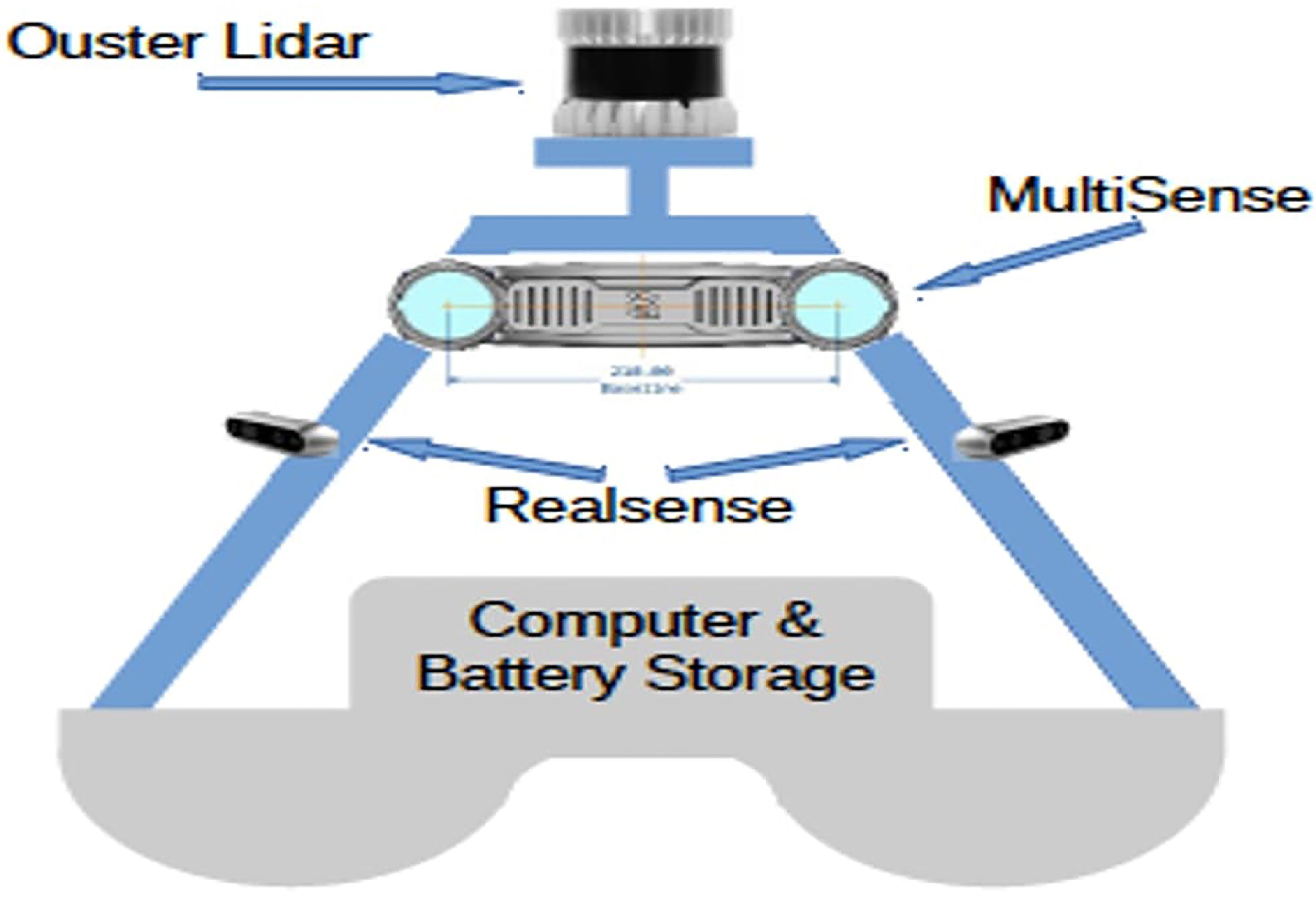
Figure 3 Placement of the sensors on the platform and which is attached to the boat.

2.4 Transforming Geodetic Coordinates of the Boat to NED Coordinates

The boat’s position information (or trajectory) is obtained from the Piksi (GPS) data in terms of its geodetic coordinates (latitude, longitude, and height). However, we need the boat trajectory in a local navigation frame. To this end, we first choose a local NED frame and transform the geodetic coordinates to NED coordinates. This transformation involves two steps as described next.

Transformation from geodetic to Earth Centered, Earth Fixed (ECEF) coordinates: Geodetic coordinates (ϕ_B, λ_B, h_B ) can be transformed to ECEF coordinates as Lugo-Cardenas et al. (2014)

$\begin{array}{ll}\left[\begin{array}{c}{X}_B\\ Y_B\\ Z_B\end{array}\right]\hspace{0.17em}=\hspace{0.17em}\left[\begin{array}{c}\left(N\left({\varphi }_B\right)+h_B\right)\text{cos }{\varphi }_B\text{cos }{\lambda }_B\\ \left(N\left({\varphi }_B\right)+h_B\right)\text{cos }{\varphi }_B\text{sin }{\lambda }_B\\ \left(\left(1-e^2\right)N\left({\varphi }_B\right)+h_B\right)\text{sin }{\varphi }_B\end{array}\right]& (9)\end{array}$

where

$$N\left({\varphi }_B\right)=\frac{a}{\sqrt{1-e^2\stackrel{2}{\sin }{\varphi }_B}}$$

which assumes that the Earth is modeled as a geodetic ellipsoid (e.g., the World Geodetic System 1984 (WGS84), the Geodetic Reference System 1980 (GRS80)), with a and e as its semi-major axis and first eccentricity, respectively.

Transformation from ECEF to NED coordinates: This can be carried out in a manner similar to the transformation from ECEF coordinates to local East-North-Up (ENU) coordinates outlined in Lugo-Cardenas et al. (2014), with simple modifications for the NED coordinates in our case. The transformation requires a reference point/position, expressed in the ECEF coordinates. Note that we take the boat’s initial position according to the GPS data (of a particular case/part) as the reference point. Also, let us denote this reference point, in terms of geodetic coordinates, as (ϕ₀,λ₀,h₀). Now, using the transformation in (9), we can obtain the corresponding ECEF coordinates as (X₀,Y_0,Z₀). Similarly, we can obtain (X_B,Y_B,Z_B) for the boat’s position given by any (ϕ_B,λ_B,h_B). Finally, (X_B,Y_B,Z_B) is transformed to the local NED coordinates as follows:

$\begin{array}{ll}\left[\begin{array}{c}{p}_{N_B}\\ p_{E_B}\\ p_{D_B}\end{array}\right]\hspace{0.17em}=\hspace{0.17em}{R}_{ECEF}^{NED}\left[\begin{array}{c}{X}_B-X_0\\ Y_B-Y_0\\ Z_B-Z_0\end{array}\right]& (10)\end{array}$

where the rotation matrix $R_{ECEF}^{NED}$ is given by

$\begin{array}{ll}{R}_{ECEF}^{NED}=\left[\begin{array}{ccc}-\text{sin }{\varphi }_0\text{ cos }{\lambda }_0& -\text{sin }{\varphi }_0\text{ sin }{\lambda }_0& \text{cos }{\varphi }_0\\ -\text{sin }{\lambda }_0& \text{cos }{\lambda }_0& 0\\ -\text{cos }{\varphi }_0\text{ cos }{\lambda }_0& -\text{cos }{\varphi }_0\text{ sin }{\lambda }_0& \text{sin }{\varphi }_0\end{array}\right].& (11)\end{array}$

It is clear from the transformation in (10) that the origin of the local NED frame is at the reference point which is same as the boat’s initial position as provided by the GPS data.

Note that we use the ‘geodetic2ned’ function in MATLAB for carrying out the transformation from geodetic to local NED coordinates in this research. This function requires the geodetic coordinates of a reference point, which we specify as (ϕ₀,λ₀,h₀). Also, out of the three NED coordinates, only the North (p_NB) and East (p_EB) coordinates are relevant for the problem at hand as we focus on the planar motion of the objects (boat and leeway). Let us define a coordinat system (or frame) with x≡p_N and y≡−p_E (i.e., x positive towards the North and y positive towards the West). This is utilized as the local navigation frame for the problem (see Supplement Figure 1). Let us denote the corresponding boat and leeway coordinate pairs as (x_B,y_B) and (x_LO,y_LO), respectively. We can recreate the entire boat trajectory provided by the GPS data in terms of (x_B,y_B) coordinates using the transformation described in this section. These (x_B,y_B) coordinates, along with the multisense camera sensor (distance) data, are then used to derive estimated leeway positions/trajectory in the local navigation frame, as described in the next section.

2.5 Calculation of Estimated Leeway Position Coordinates

The distance data obtained from the machine learning analysis (identification and estimation) are regarded as pseudo range measurements with respect to the boat. Thus, we have the following mathematical relationship:

$\begin{array}{ll}r=\sqrt{{(x_{LO}-x_B)}^2+{(y_{LO}-y_B)}^2}& (12)\end{array}$

where r is the distance or pseudo range (see Supplement Figure 1). The objective is to find estimates of the pair (x_LO,y_LO) utilizing the knowledge of (r, x_B, y_B ). These estimates are obtained by solving the following unconstrained optimization problem:

$\begin{array}{ll}\underset{x\in ℝ, y\in ℝ}{\min }\hspace{0.17em}{\left(\left({(x-x_B)}^2+{(y-y_B)}^2\right)-r^2\right)}^2.& (13)\end{array}$

The above cost function is locally convex, which is illustrated in the plots in Supplement Figure 2. Therefore, existing convex optimization solvers would generally require a carefully specified initial guess for the solution to successfully solve this problem. To this end, the initial guess for the solution is taken as

$$x^{\left(0\right)}=x_B+r\hspace{0.17em}\text{cos }(\theta ), y^{\left(0\right)}=y_B+r\hspace{0.17em}\text{sin }(\theta )$$

where θ = θ_B + θ_C is the camera angle with respect to the positive x axis of the local navigation frame, with θ_B as the boat heading angle and θ_C as the camera angle with respect to the surge direction (see Supplement Figure 1). Note that the optimization problem (13) is solved using the ‘fmincon’ function in MATLAB, with a primal-dual interior-point algorithm (Supplement Data for the details).

2.6 Test Data Collection

Four continuous drift runs were conducted on two drifting objects on 18 April 2021, from 14 p.m. GMT to 21 p.m. GMT, with the support of the USCG (auxiliary) vessel in Galveston Bay (located at 29.34N, -94.85W) (Figure 4). The drifting objects that were used in this study were pelican rectangular boxes (pelican-1 and pelican-2) (Table 1). We conducted two tests on the pelicans. We also used two full-size mannequins resembling PIWs. The first was referred to as PIW-1, and the second, onto which holes were drilled so it would be partially submerged in water, was referred to as PIW-2. The experiments were conducted in the following manner. The objects were deployed from the boat at different locations in the 5-mile vicinity of the coordinates 29.34N, -94.85W. The objects drifted due to the combined action of the wind and the waves, and the sensor data were recorded for the entire duration of the experiment. The boat fitted with the operational sensing platform followed the drifting object within a 5-mile radius from the object. The moving sensing platform (boat) gathered real-time data through the LiDAR sensor, two multisense (MS) depth cameras (MS1 and MS2), GPS, and IMU. Simultaneously, the wind anemometer fitted onto the poles of the boat collected the local wind data. At the beginning of the experiment, the current profiler for measuring the current speed was deployed at the start location. It was retrieved at the end of the experiment. The start and end times of each test case were recorded, and the outputs of the LiDAR sensor were collected in the form of bag files, the outputs of the cameras were stored as image files, the data from the GPS were stored as ROS files, and the wind and ocean data were retrieved as text files. All these data were stored on the onboard computer. Figure 5 shows the LiDAR image on the right panel and the images from the left and right MS cameras on the upper and lower parts of the left panel, respectively. The object was 60m from the sensor, and as it was outside the range of the left MS, it could be seen only in the right MS. Using the information from the right MS camera and the LiDAR sensor, we calculated the distance of the object from the sensor.

FIGURE 4

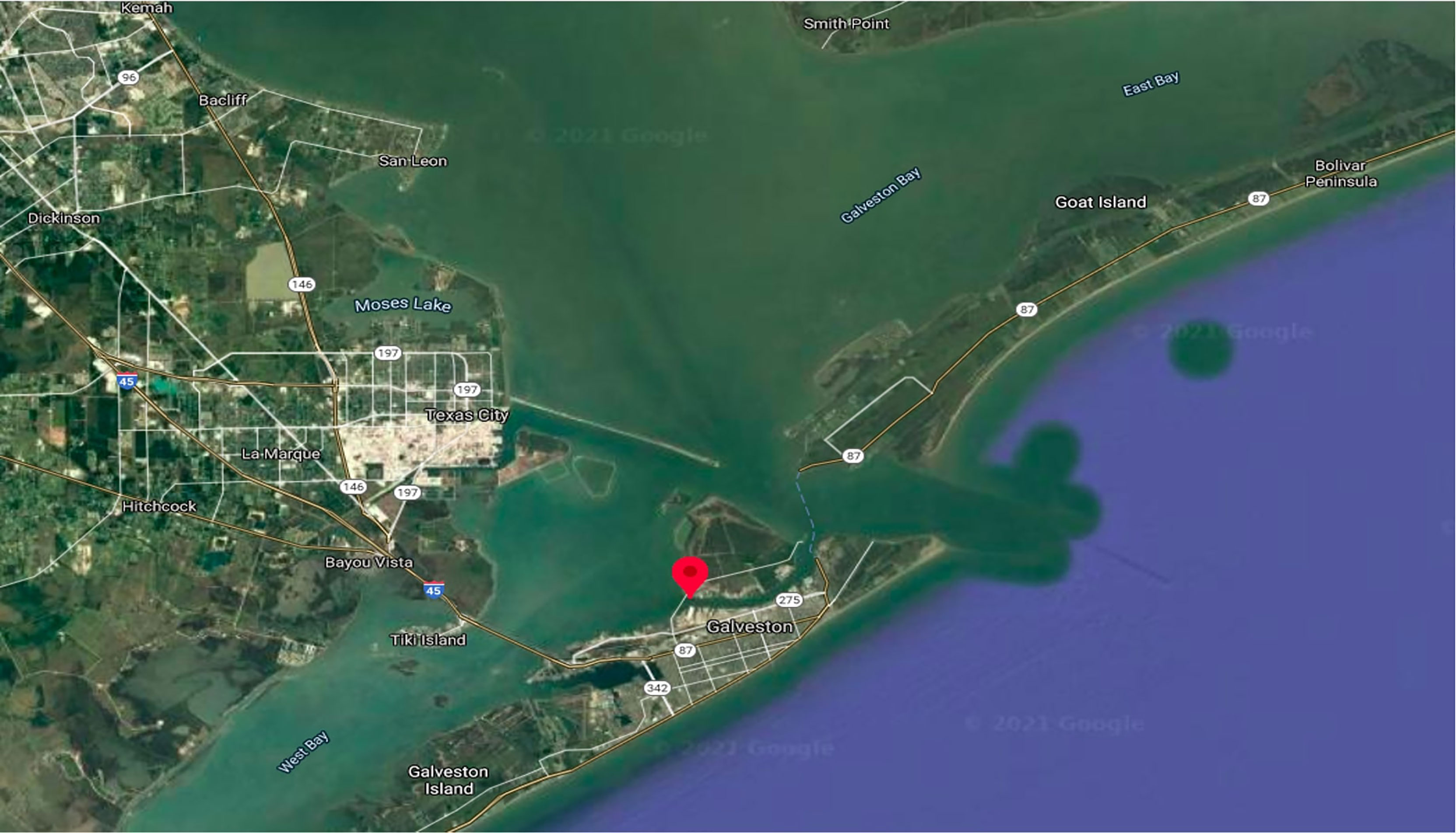
Figure 4 Location of the field test for data collection. At the docking area, the data-collection platform was fitted on the boat. The boat was steered 5 miles inside the bay and the objects were deployed.

FIGURE 5

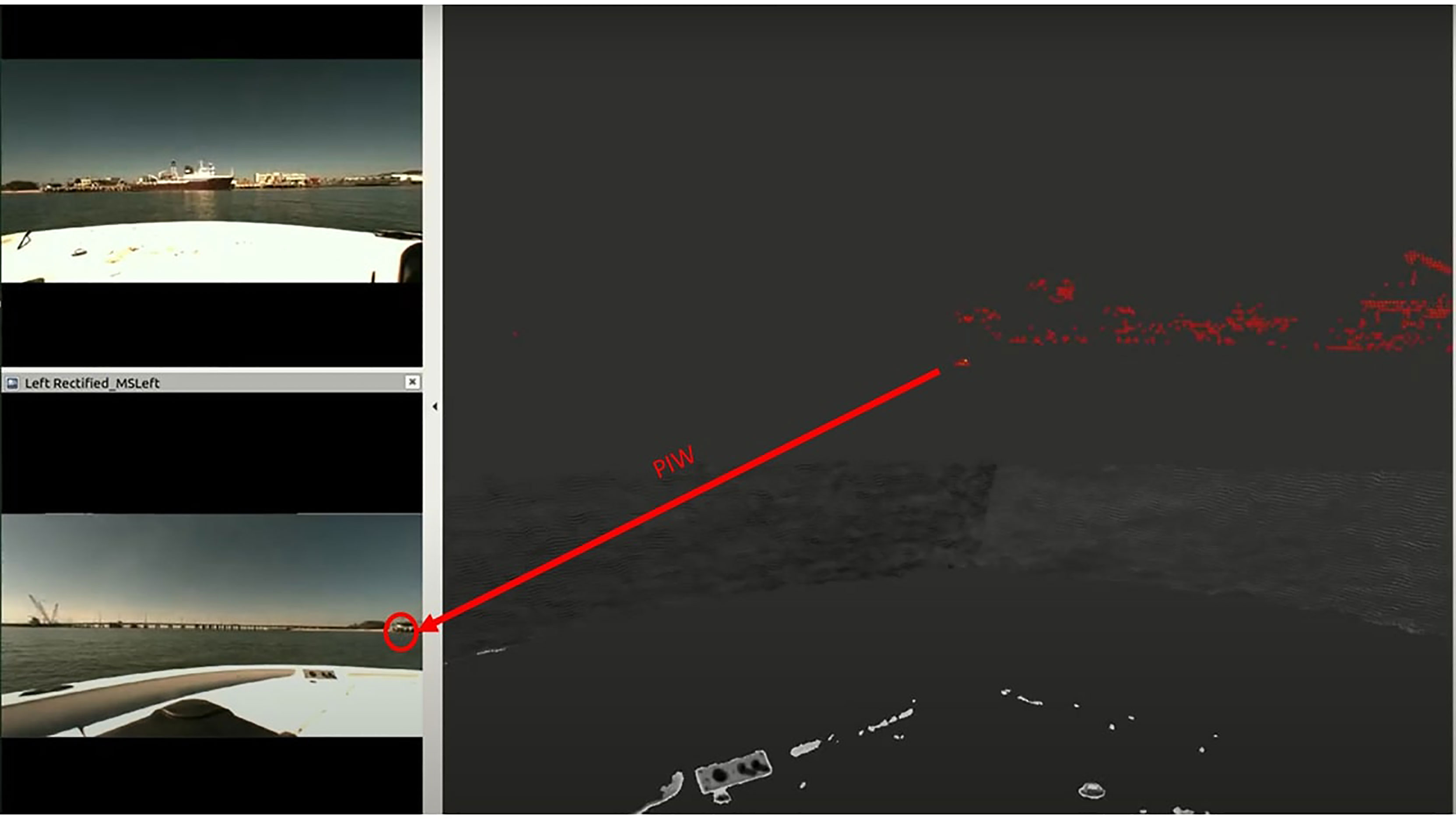
Figure 5 [Top Left] Image from the left stereoscopic camera MS1, [Lower Left] Image from the right stereoscopic camera, MS2, [Right] Output from the LiDAR bag files.

TABLE 1

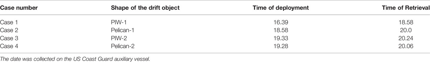
Table 1 Test conditions for the 4 test cases conducted in Galveston bay at 29.34 N, -94.85 W.

3 Results

In this section, the results of the sensors’ data collection, the machine learning analysis for object detection and tracking, and the drift analysis are presented. The object detection, tracking, and distance mapping results are discussed first, followed by the results of the analysis of the leeway objects’ drift characteristics.

3.1 Object Detection and Tracking

The data for training the models were collected in two steps. The first set of data were collected from the swimming pool of the University of Texas, San Antonio (UTSA), and the second set of data were collected during the field testing in Galveston Bay, Texas. The data collected from the swimming pool revealed high-level features at close range (for the objects, see Figure 6). The second set of data were collected to capture the low-level features in a long-range setup, where the objects were directly affected by the ocean conditions (see Figure 7).

FIGURE 6

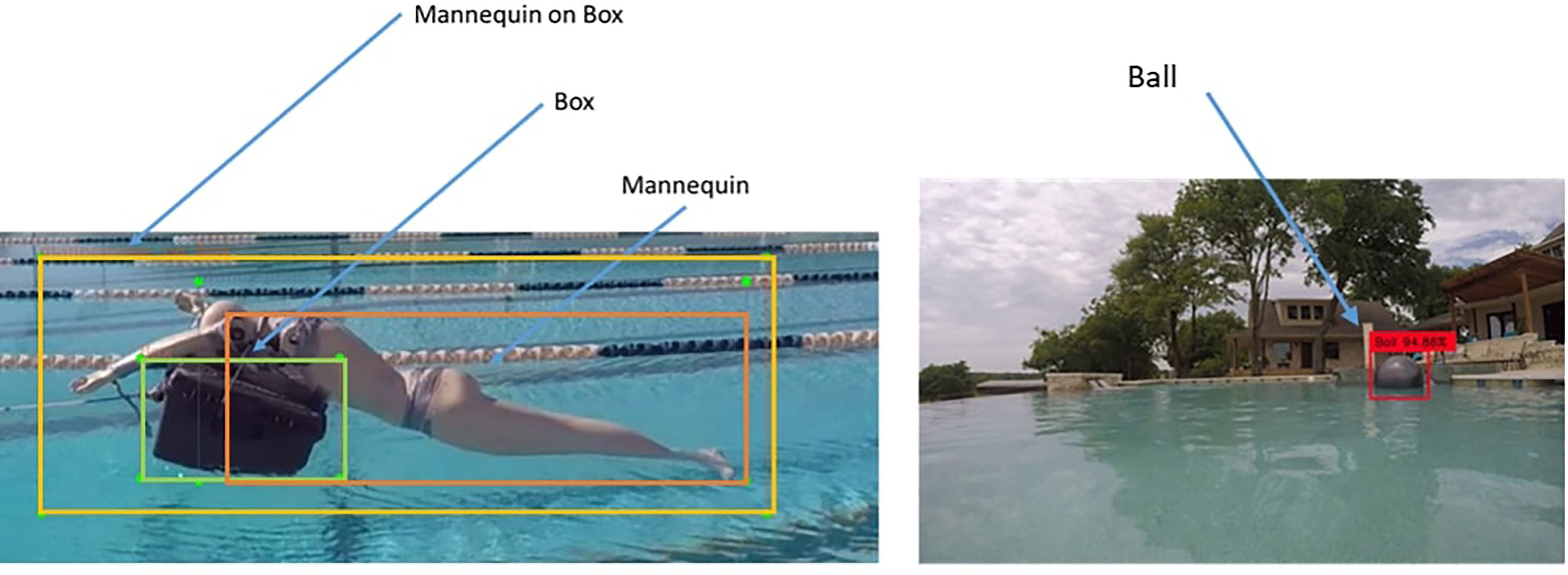
Figure 6 Labels for training the object detection model: [Left Panel] To replicate PiW we utilized a mannequin. In addition we also labelled a box and a combination of mannequin on box to show the PiW is using a support to keep themselves afloat, [Right Panel] label to identify spherical shaped object in this case a ball.

FIGURE 7

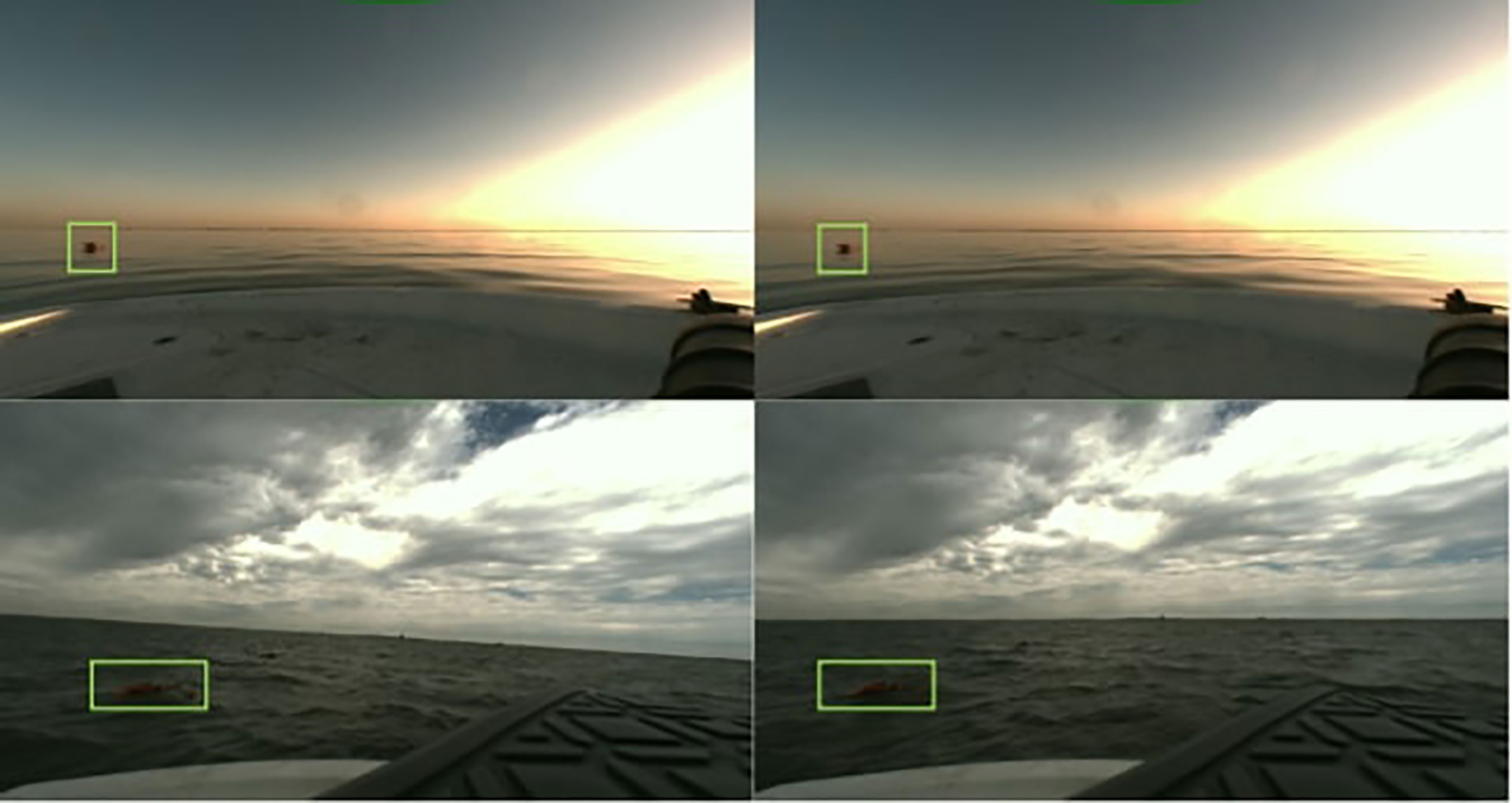
Figure 7 Results of the object tracking algorithm where detection is done once and tracking is used to detect the object for the rest of the frames [Top left] Object detection module is used to detect the object of interest (Pelican). [Top Right]. Detected object is tracked in the next frame [Lower Left] The detection algorithm detects the object in the frame [Lower Right] tracking the object after 40.

frames.

Figure 6 shows the labels used to train the detection model. Four labels with three distinct objects were created. The labels are Box, Ball, Mannequin, and Mannequin on the box. The collected data were separated into train and test sets to train and estimate the performance of the trained model. A pre-trained YOLO model [trained on COCO dataset Lin et al. (2014)] was used as the base and we further fine-tuned the model utilizing the training data. Table 2 shows the mAP performance of the model on the test data. The test data consists of objects of interest under different case scenarios with varying degrees of object immersion in water for pelican box, and with different surrounding wave intensity and lighting conditions while floating in the water. On the test data, the detection model has a >99% accuracy for detecting the basic shapes like box and ball. Wheres, the detection performance falls to 72.4% for the mannequin. A combination of mannequin and box has a higher detection rate with the limited number of samples in the data (153 data samples.) The mAP for all the objects is calculated to be 89.65% which can be considered very good performance for the case in hand. We hypothesize the model performance can be improved by increasing the training data for the diversity of objects. We had to limit our labeling and data collection steps due to time constraints.

TABLE 2

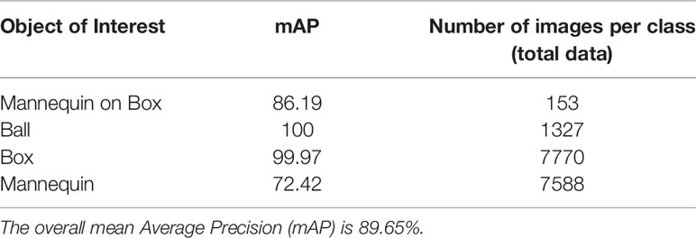
Table 2 The average precision for different objects.

We also set up additional tests to check the model’s capabilities and performance under different test conditions. The test setups are as follows-

3.1.1 Detection and Tracking Capability in Different Degrees of Immersion

As shown above, the trained model does an excellent job detecting our objects of interest (see Table 2). Now, we set the object of interest at different degree immersion settings to check how the trained model performs. The detection model identifies objects perfectly under 0%, 25%, and 50% immersion consecutively. An interesting observation is for the above-mentioned immersions the detection model performs well regardless of the object is closer to the camera or not but the difference can be noticed for immersion at 75%. When the object is closer to the camera the model can detect it clearly but when the object of interest is far away from the camera the trained model fails to detect the object. Among the test cases with 75% immersion, we achieved an accuracy of 67.5% while all the failed case falls into objects located far away from the camera. Supplement Figure 4 shows some of the sampled results from the detection test at different immersion levels.

3.1.2 Detection and Tracking Capability in Continuous Setup (Monitoring)

The combination of detection and tracking algorithm is very robust. The detection algorithm identifies the object at the first frame and records the object features. The tracking algorithm then tracks the features in corresponding frames. In Figure 8 top left image shows the detected object. The following two frames (left to right) continue to detect the object. In frames 4 and 5 the object detector re-detects the objects. An interesting observation is that the model detects the object as both mannequin and box but as the model has a lower certainty level (middle row left frame) for the detected object to be a box, it drops that label and continues to detect it as a mannequin. The consecutive frames continue to track the detected object. And thus the test continues till the process is terminated. We ran a 6 (six) hour test to check the performance of the model. The result from the test can be found in this compressed video link https://drive.google.com/file/d/18YXTWANDR5SbiLgfu7MK1qR-Id61D_uz/view?usp=sharing.

FIGURE 8

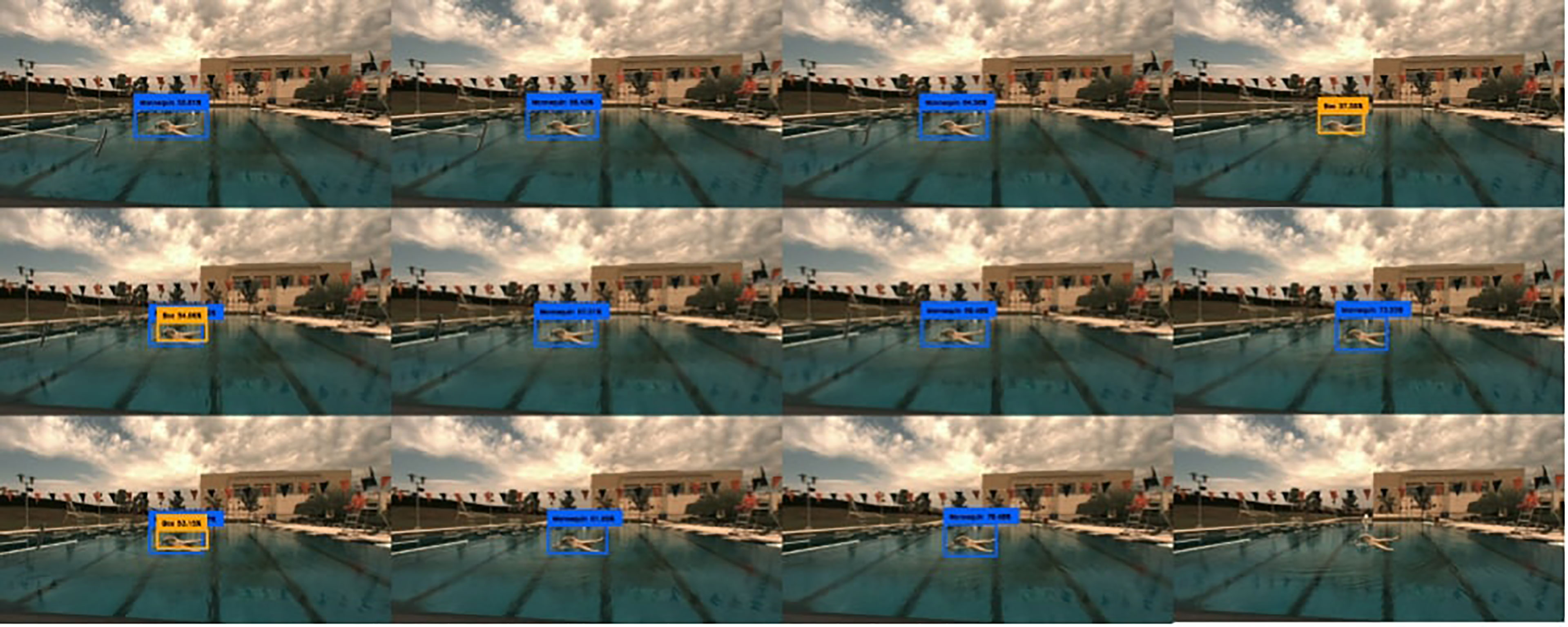
Figure 8 Continuous detection and tracking performance of the proposed model.

3.1.3 Detection and Tracking Capability in Different Lighting Conditions

We further tested the model performance under different lighting conditions (both in Galveston and UTSA pool). Supplement Figure 4 shows a few sampled images from the test data where the object of interest is at different lighting conditions. The top left image of Supplement Figure 4 shows the object of interest in the frame when the sun is perpendicular to the camera thus distorting the field of view. The top right image shows the object in a sunset lighting condition, the bottom left shows a cloudy sky when the test was conducted and the bottom right shows the object under a clear and bright lighting condition. In all the lighting conditions the proposed model was able to detect and track the objects.

For all the field tests, all the objects were detected and tracked with a very high degree of accuracy. It should be noted that when the object reappeared after being completely submerged or drifted away in water for a short period of time, the algorithm was still able to detect it. Further, during the field tests, there were many ships and other natural obstructions in the test area. In-spite of the presence of these objects in the vicinity of the test site, the machine learning algorithm accurately detected and tracked the target object.

3.2 Distance Mapping

To map the location of the object of interest with respect to the location of the camera we utilize the methodology introduced in section 2.2.3. Using the rectified stereo images collected from the camera we use PSMNet to map the distances of the objects in the area of focus. The calibration of the model was performed in an in-house test-bed where the box/pelican was set at different distances to determine the baseline distance of the camera. Figure 9 shows the estimated map using PSMNet and on top shows the distance of the object from the camera in meters (both the maximum possible distance and average distance). To speed up the process of determining the distance of the object of interest, we only generate the distance map of the region of the identified object in the image. The region is retrieved from the object detection and tracking module. Then we map the distance of the proposed region using the proposed model. The processing time per frame is shown in section 3.3. A short video of full mapping can be found here: https://drive.google.com/file/d/1lQd7X9HD3By8zN-0R9-aynIJ72fnLAqi/view?usp=sharing.

FIGURE 9

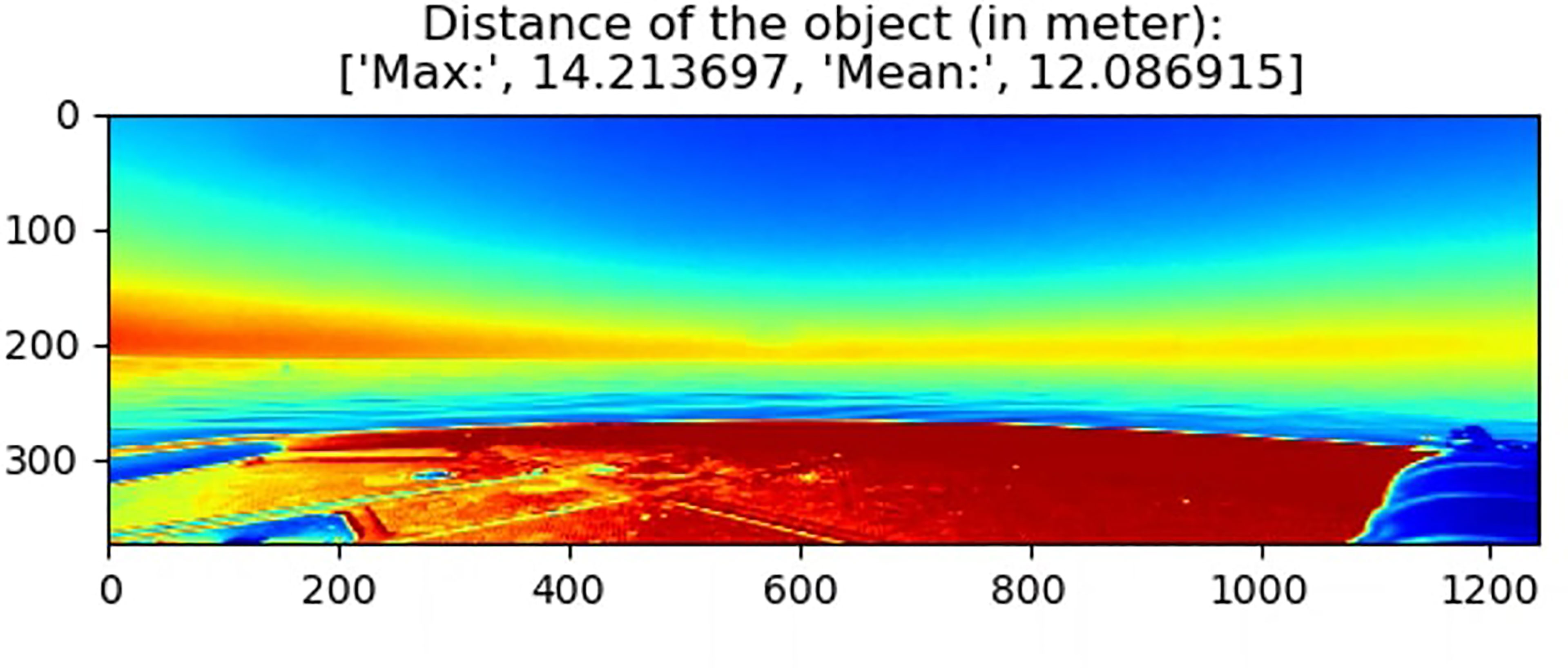
Figure 9 Distance mapping from stereo images.

3.3 Time Analysis of Machine Learning Algorithm

Time analysis of the detection, tracking, and distance mapping modules are performed in a real-life deployment. The test was performed for a six hour test in a Galveston. The summary of time is as follows-

1. Detection and Tracking:

a. Pre-detection processing: 0.8 sec/frame (on average. Max: 1.5 sec/frame)

b. The detection time: 1.53 sec/frame (on average. Max: 2.73 sec/frame)

2. Depth Estimation:

a. Pre-range calculation processing: 0.3 sec/frame (on average. Max:.7 sec/frame)

b. The range calculation: 4.71 sec/frame (on average. Max: 7.39 sec/frame)

The total average time when considered best case scenario is 7.34 sec/frame and the worst case scenario is 12.32 sec/frame.

3.4 Drift Analysis

Leeway drift is defined as the movement of a leeway object relative to the ocean’s surface (Allen and Plourde, 1999). The location of the leeway is the result of the leeway drift and the movement of the upper layer of the ocean. As leeway is influenced by the wind forces and ocean currents, it may not be aligned with the wind and with a component of the leeway velocity (L) along the wind direction (DWD), and with the component perpendicular to the wind drift (CWD), as shown in Figure (Supplement Figure 1). When there is no wind, objects will move with the ocean current. However, when wind is present, it has two effects. First, the shear stress at the water/air interface creates waves and alters the surface current. Second, the wind acting on the exposed surfaces of the object generates leeway drag. It should be noted that the leeway velocity also depends on the degree of immersion of the object below the ocean’s surface. The object will be influenced by the aerodynamic forces on the parts exposed to the wind and will be influenced by the oceanic forces on the submerged parts. The deviation of the leeway drift from the downwind direction is referred to as the leeway divergence (L_α), and it is calculated using the leeway angle, which is defined as the angle between the wind direction and the direction of the leeway velocity. To calculate the leeway drift, we used the distance of the leeway from its last known location and estimated it using the mean leeway speed during that time.

Accurate determination of the divergence of leeway objects from the downwind direction is very important for SAR operations. The proposed framework can be used to calculate the leeway divergence on the basis of the downwind and crosswind components of the leeway. Here, the depth maps can be used to determine the distance of the leeway from the sensor. The local wind speed (W_s) and the ocean current speed (C_s) are measured using the wind anemometer and current profiler, respectively. Like Breivik and Allen (2008), we defined leeway speed (L) as the magnitude of the leeway velocity. The (x, y) coordinates of the leeway trajectory are determined in real time. Using this information, the components of leeway velocity along the N-S and E-W directions are calculated, and the leeway speed is also calculated as the magnitude of the components along the E-W and N-S directions. Leeway angle (L_α) is defined as the leeway drift direction minus the downwind direction, which is either positive or negative, with a deflection clockwise or counterclockwise from the downwind. Leeway speed and leeway angle are the components of the leeway velocity vector expressed in polar coordinates. DWL and CWL, on the other hand, are the components of the leeway velocity vector expressed in rectangular coordinates. The slopes of the DWD and LWD coefficients are defined as DWD/Ws and LWD/Ws, respectively. Divergence angle is a key parameter of the leeway characteristics and is calculated as DA = arctan(CWL/DWL).

Figure 10 shows the data from the Tides and Currents website of the National Oceanic and Atmospheric Administration (NOAA), developed and supported by the Center for Operational Oceanographic Products and Services. The wind and ocean current data at the Galveston Bay entrance (29.34N, 94.56W) and at the Galveston Bay west end (29.14N, 95.045W) were recorded. These locations were 28 and 29 km away from the test site, respectively. To a certain degree of accuracy, the data can serve as reliable validations. On the day of the experiments, a maximum wind speed of 10 m/s was recorded at the site, and the gusts varied significantly from 11.8 m/s in the morning to 13.39 m/s in the afternoon and 10 m/s in the evening. The average wind speed for the experiments was recorded as 6.3/7.14 m/s for the pelican/PIW tests. The ocean current data were highly intermittent, 0.15 m/s on average. The data collected from the current profiler ranged from 0.1 m/s to 1.7 m/s, with an average (over the bins) of 0.3 m/s. The data for the entire duration of all the experiments were averaged.

FIGURE 10

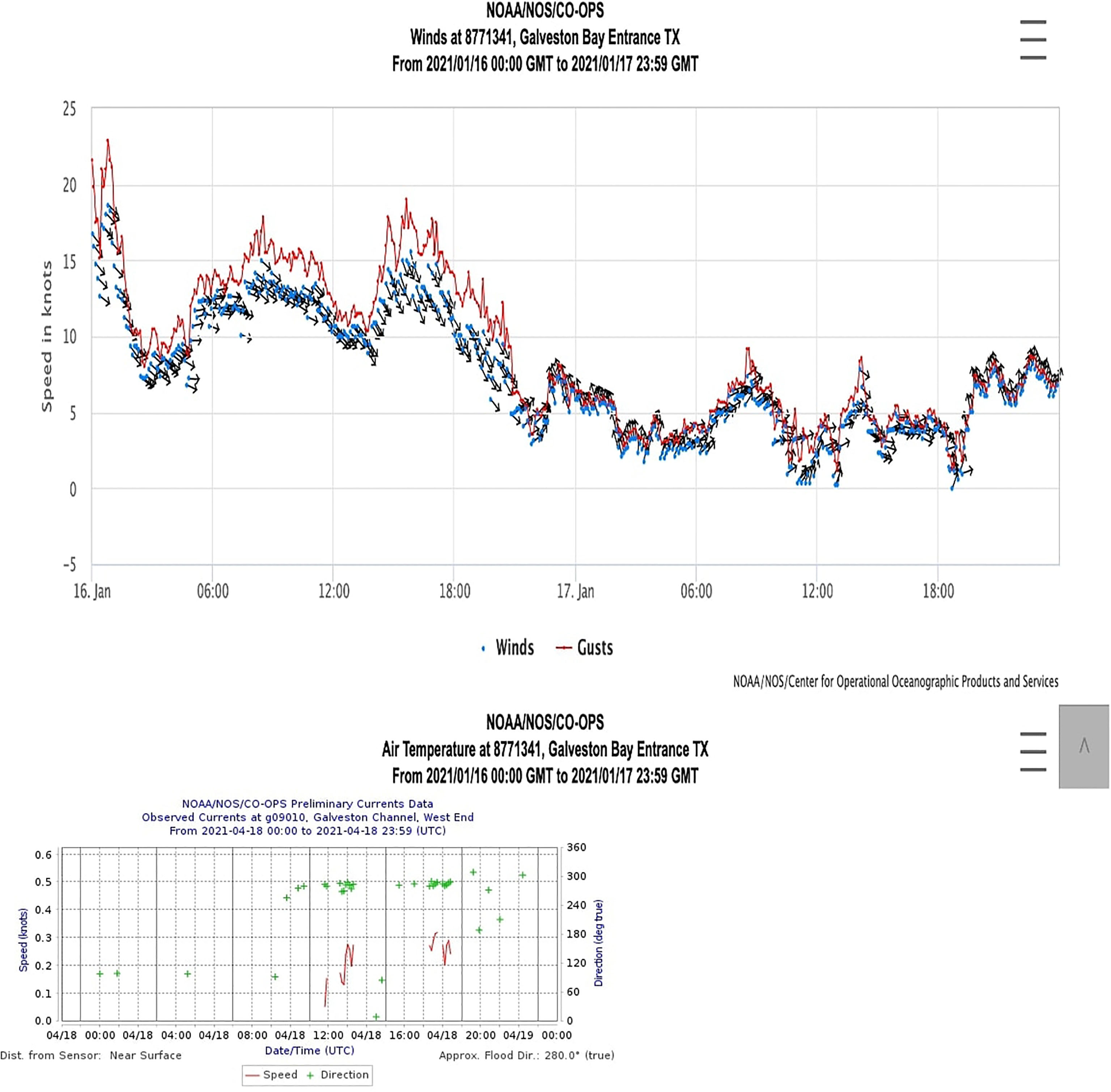
Figure 10 Validation of the nearby meteorological and oceanography data.

The results of the analyses for the four cases are presented in Table 3. The average wind speed was obtained by averaging the speed of the wind for the entire duration of the experiment. For the pelican-1 experiment, the average wind speed was 7.14 m/s, the average current speed was 1.68 m/s, the average leeway speed was 0.75 m/s, the DWL and CWL slopes were both 0.06, and the divergence angle was -26°. For the PIW experiments, PIW-2 had an average wind speed of 6.3 m/s, which resulted in an average leeway speed of 1.07 m/s, with a 16° divergence angle. As the wind speed increased to 6.6 m/s, the leeway speed increased to 1.25 m/s, with an 80° divergence angle.

TABLE 3

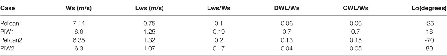
Table 3 Calculation of the drift characteristics for the cases.

Figure 11 shows the trajectory of the leeway object for the four cases. For the first pelican case (pelican-1), the trajectory was almost linear in the S-W direction. For the second pelican case (pelican-2), the initial drift of the leeway was in the S-W direction, and it continued to drift in the S-direction. For the first PIW case (PIW-1), the leeway initially drifted in the S-E direction and then switched its drift direction to S-W. The second PIW (PIW-2) had a more complicated trajectory. For the four cases, the average wind speed varied in the 6.3–7.14 m/s range, and the leeway speed varied in the 0.75–1.32 m/s range. The slope of the leeway speed was in the 0.1–0.2 range for the four classes. Figure 12 shows the maps of the crosswind-downwind distance travelled by the leeway. The CWL and DWL distances were calculated using the crosswind and downwind velocity components, respectively, during the experiment. For pelican-1, the drift was in the S-W direction, with a mean divergence angle of -25°. The map of the CWL-DWL distance shows a consistent trend, with a significant downwind drift with rightward divergence (20–25°in the eastward direction). For pelican-2, there was initially a significant downwind drift, but the crosswind drift component later became dominant, and it drifted in both the positive (eastward) and negative (westward) directions to the downwind, with a mean divergence angle of -70°, suggesting a mean skewed drift westward. The CWL-DWL distance maps for PIW-1 and PIW-2 are shown in the lower panels of Figure 12, respectively. The drift of PIW-1 was mostly downwind, in the S-W direction, and the mean divergence angle was around 16°. The trajectory of PIW-2, on the other hand, was much more complicated, and the drift angle varied from -110° to +120°, with a mean drift angle of 80°. The wind direction varied throughout the experiment.

FIGURE 11

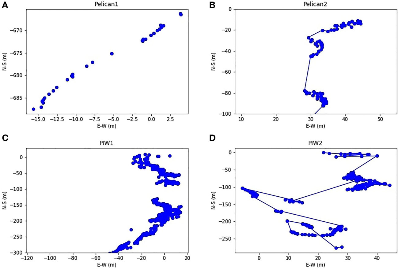
Figure 11 Trajectory of (A) Pelican 1 in m (B) Pelican 2 in m, (C) PIW 1 in m. (D) PIW 2 in m.

FIGURE 12

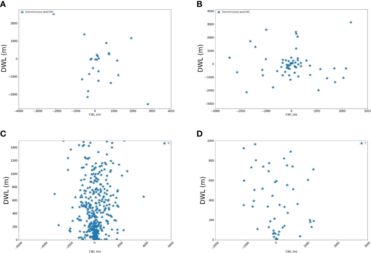
Figure 12 CWL-DWL trajectory plots for (A) Pelican 1 in m (B) Pelican 2 in m, (C) PIW-1 in m. (D) PIW 2 in m.

Overall, for the pelican cases, which were mostly floating over the water, the wind played an important role, with the drift significantly in the downwind direction. When the wind speed had been reduced for pelican-2, the relative effect of the current became dominant, with a higher leeway divergence angle compared to pelican-1. For PIW-1, which was a buoyant mannequin, the wind effects were also dominant, with the drift mostly in the downwind direction, whereas for PIW-2, which was the partially submerged mannequin, the percentage of the body immersed in the water varied significantly throughout the drift test, and the drift alternated between the downwind and crosswind drifts. For floating objects dominated by form drag, such as pelicans, using the slope of DWL will provide a good estimate of the drift divergence and drift velocity. The PIWs exhibited a similar trend when they were completely floating in water. When the PIW was partially submerged in water, the prediction of the drift and divergence was very complicated, and the average slope of DWL and CWL (over the entire duration of the experiment) did not prove to be an accurate estimate, and there was a need to calculate the slope in real time. For such cases, our proposed method of calculating the drift coefficients in real time is extremely valuable.

Conclusions

A novel method of obtaining the leeway drift and divergence characteristics in real time using a moving platform with vision-based sensors and machine learning techniques was developed. The system level architecture is discussed in detail herein. A platform consisting of an Ouster OS128 LiDAR sensor, MS stereoscopic depth cameras, a GPS, an IMU, a wind anemometer, and a centralized computing station was designed and built at the Laboratory of Turbulence, Sensing and Intelligence Systems of UTSA. The ocean current speed is calculated by a Nortek Eco ADCP current profiler. A wind anemometer attached to the poles of the boat collects the wind speed and direction data. The onboard computer collects the data from the sensors in real time. The localization module provides the location of the moving platform. A transformation algorithm is used to convert the location of the drifting object in the frame of the moving platform to a geostationary frame of reference. After the successful integration of the data from the sensors, the machine learning technique is used to determine the shape and location of the detected object. The system was trained to identify objects with the shape of a rectangular box (pelican) or a PIW, and to identify spherical objects (circular tanks). The training for object detection was performed in two steps. The first set of data was collected from the swimming pool at UTSA, and the second set of data was collected during the field tests in Galveston Bay. The advantage of this two-step approach is that the data collected from the swimming pool provide information regarding the high-level features at a close range, and the second set of data collected during the field tests capture the low-level features in a long-range setup, where the ocean currents and waves directly influence the objects. The performances of the models were measured using the mAP metric. The model detected PIW with a mAP of 72.42% and a pelican box with a mAP of 99.37%. The results from the data collected during the field tests in the Galveston region in Texas, USA are reported herein. Four continuous drift runs were conducted on four different drifting objects (pelican-1, pelican-2, buoyant PIW, and partially submerged PIW). The objects were deployed from a USCG auxiliary boat. The hardware platform that had been constructed at UTSA was first fixed on the boat. The Nortek Eco ADCP was deployed in water at the beginning of the first experiment and was collected at the end of the last experiment. The objects were deployed from the boat at different locations in the 5-mile vicinity of the coordinates 29.34N, -94.85W. The objects drifted due to the combined action of the wind and the waves, and the sensor data were recorded for the entire duration of the experiments. The leeway drift is caused by the combined action of the aerodynamic forces due to the wind and of the hydrodynamic forces due to the current Brushett et al. (2017). The wind speed, wind shear, and turbulence together influence the aerodynamic forces. Hence, using an analytical or numerical modeling approach to account for the aerodynamic forces is very challenging as measuring the wind shear, wind turbulence, and ocean waves is prone to many errors. In most of the previous studies, the aerodynamic forces were characterized on the basis only of the wind speed. In this study, an alternative approach was used to calculate the drift characteristics. Machine learning algorithm was used on the data collected from the cameras to detect a drifting object and to map their distance with respect to the boat. The method eliminates the need to calculate the aerodynamic/hydrodynamic forces to obtain the object trajectory. After the machine learning algorithm and localization steps, the leeway location in the (x,y) or (lat,lon) coordinate system is measured in real time. The rate of change of the location is calculated to obtain the leeway velocity and direction. The wind speed and direction are also measured, and the components of the leeway velocity in the wind direction (DWL) and perpendicular to the wind direction (CWL) are calculated. The divergence angle is also calculated as the difference between the leeway direction and the wind speed direction. The measured wind speed was validated using the NOAA measured data at a location 25 km from the experimental site. The magnitudes cannot be compared, but the accuracy of the measurements can be qualitatively estimated.

The distance maps of CWL-DWL for the four cases showed significant differences between the four scenarios. Pelican-1 drifted in the S-W direction. During this time period, the wind direction changed from S-E to S-W and vice versa. The mean divergence angle of the pelican was 25° westward. For pelican-2, the winds were mainly in the S-E direction, and the pelican drifted to the left by 70°, resulting in a drift in the S-direction. The DWL slopes for pelican-1 and pelican-2 were 0.1 and 0.2, respectively, and the LWL slopes were 0.06 and 0.15. As can be seen in the trajectory maps, the CWL component dominated pelican-2, with a much higher divergence angle than pelican-1. The influence of the ocean current was higher on pelican-2. The drift was more complicated for the PIWs. The initial drift of PIW-1 was in the S-E direction, and after drifting almost 200 m from the initial location, it changed direction to S-W and drifted 100 m in such direction. The drift of PIW-2 was extremely complicated as it changed directions and slopes multiple times during the experiment. PIW-2 was the partially submerged PIW, where the amount of immersion varied throughout the drift run; hence, it was influenced by the wind and ocean currents to varying degrees, which was not constant for the entire duration of the experiments. As for PIW-1, its average DWL slope was 0.7, and its mean divergence angle was 16°.

This work has an important contribution to the real-time detection of moving objects in nonlinear, dynamic environments, providing a viable alternative to the expensive and complex numerical simulations for determining the drift characteristics of drifting objects as it is less costly and eliminates the need to approximate the environmental conditions in the calculations, which is always a challenge. The proposed method is very suitable for complex cases, such as for PIWs partially submerged in water, where the degree of immersion changes significantly over time and the influence of the wind/ocean forces on the drift characteristics thus varies. In the future, we will extend this technology for use in unmanned boats.

Data Availability Statement

The original contributions presented in the study are included in the article/Supplementary Material. Further inquiries can be directed to the corresponding author.

Author Contributions

KB was responsible for the overall writing, organization and drift analysis. PK was responsible for the hardware implementation and sensor calibration along with writing the hardware platform section, AA and SHAF was responsible for implementing the machine learning algorithm and writing the corresponding part. DB was responsible for implementing the transformation, analysis. All authors contributed to the article and approved the submitted version.

Funding

Funding have been received from the Minority Serving Institutions Science, Technology, Engineering and Mathematics Research and Development Consortium (MSRDC) as a subaward #D01_W911SR-14-2-0001 from Department of Homeland Security. Thanks to USCG Research Division team for their technical guidance. KB acknowledges support from NASA Center for Advanced Measurements in Extreme Environments, Grant 80NSSC19M0194.

Conflict of Interest

The authors declare that the research was conducted in the absence of any commercial or financial relationships that could be construed as a potential conflict of interest.

Publisher’s Note

All claims expressed in this article are solely those of the authors and do not necessarily represent those of their affiliated organizations, or those of the publisher, the editors and the reviewers. Any product that may be evaluated in this article, or claim that may be made by its manufacturer, is not guaranteed or endorsed by the publisher.

Acknowledgments

The opinions, analysis and conclusions presented in this paper are the authors scientific viewpoints and it does not reflect the viewpoints of USCG RDC team. The authors acknowledge the support from USCG Research and Development Center throughout the project. It would not have been possible to conduct this work without their support. The authors acknowledge USCG for connecting us with the US coast Guard auxiliary services who have helped us with the data collection. The data was collected in USCG auxilary service boat. The authors acknowledge the funding from Department of Homeland security through MSRDC. The authors acknowledge the NASA CAMEE for providing the computational resources.

Supplementary Material

The Supplementary Material for this article can be found online at: https://www.frontiersin.org/articles/10.3389/fmars.2022.831501/full#supplementary-material

Footnotes

1. ^ Disparity refers to the horizontal displacement between a pair of corresponding pixels from a fixed frames left and right camera image.

References

Akhtar M. R., Qin H., Chen G. (2019). “Velodyne Lidar and Monocular Camera Data Fusion for Depth Map and 3d Reconstruction,” in Proceedings of the Eleventh International Conference on Digital Image Processing (ICDIP 2019), International Society for Optics and Photonics, Guangzhou, China, May 10th to 13th, 2019, Vol. 11179. 111790E.

Google Scholar

Allen A., Plourde J. (1999). “Review of Leeway: Field Experiments and Implementation,” in Report CG-D-08-99, US Coast Guard Research and Development Center, Groton, CT, USA CG-D-08-99 (US Coast Guard).

Google Scholar

Behrendt K., Novak L., Botros R. (2017). “A Deep Learning Approach to Traffic Lights: Detection, Tracking, and Classification,” in 2017 IEEE International Conference on Robotics and Automation (ICRA) (NJ, US: IEEE), 1370–1377.

Google Scholar

Biswas J., Veloso M. (2012). “Depth Camera Based Indoor Mobile Robot Localization and Navigation,” in Proceedings of the 2012 IEEE International Conference on Robotics and Automation, 1697–1702. (NJ, US: IEEE).

Google Scholar

Breitenstein M. D., Reichlin F., Leibe B., Koller-Meier E., Van Gool L. (2010). Online Multiperson Tracking-by-Detection From a Single, Uncalibrated Camera. IEEE Trans. Pattern Anal. Mach. Intell. 33, 1820–1833. doi: 10.1109/TPAMI.2010.232

PubMed Abstract | CrossRef Full Text | Google Scholar

Breivik O., Allen A. (2008). An Operational Search and Rescue Model for the Norwegian Sea and the North Sea. J. Mar. Syst. 69, 99–113. doi: 10.1016/j.jmarsys.2007.02.010

CrossRef Full Text | Google Scholar

Brushett B., Allen A., King B., Lemckert T. (2017). Application of Leeway Drift Data to Predict the Drift of Panga Skiffs: Case Study of Maritime Search and Rescue in the Tropical Pacific. Appl. Ocean. Res. 67, 109–124. doi: 10.1016/j.apor.2017.07.004

CrossRef Full Text | Google Scholar

Buchman S. (2020). United States Coast Guard.” Annual Performance Report United States Coast Guards. Unite. States Coast. Guard. Rep.

Google Scholar

Cesic J., Markovic I., Juric-Kavelj S., Petrovic I. (2014). Detection and Tracking of Dynamic Objects Using 3d Laser Range Sensor on a Mobile Platform. In 11th International Conference on Informatics in Control, Automation and Robotics (ICINCO). Vol. 2, 110–19. (NJ, US: IEEE)

Google Scholar

Chang J. R., Chen Y. S. (2018). “Pyramid Stereo Matching Network,” in Proceedings of the IEEE Conference on Computer Vision and Pattern Recognition Cameras. (NJ, US:IEEE).

Google Scholar

Chen L. C., Papandreou G., Kokkinos I., Murphy K., Yuille A. L. (2017). Deeplab: Semantic Image Segmentation With Deep Convolutional Nets, Atrous Convolution, and Fully Connected Crfs. IEEE Trans. Pattern Anal. Mach. Intell. 40, 834–848. doi: 10.1109/TPAMI.2017.2699184

PubMed Abstract | CrossRef Full Text | Google Scholar

Crowley J., Demazeau Y. (1993). Principles and Techniques for Sensor Data Fusion. Signal Proc. 32 (1–2), 5–27. doi: 10.1016/0165-1684(93)90034-8

CrossRef Full Text | Google Scholar

Davidson F., Allen A., Brassington G., Breivik B. (2009). Applications of Godae Ocean Current Forecasts to Search and Rescue and Ship Routing. Oceanography 22, 176–181. doi: 10.5670/oceanog.2009.76

CrossRef Full Text | Google Scholar

De Silva V., Roche J., Kondoz A. (2018a). Fusion of Lidar and Camera Sensor Data for Environment Sensing in Driverless Vehicles. Loughborough University https://hdl.handle.net/2134/33170.

Google Scholar

De Silva V., Roche J., Kondoz A. (2018b). Robust Fusion of Lidar and Wide-Angle Camera Data for Autonomous Mobile Robots. Sensors 18, 2730. doi: 10.3390/s18082730

CrossRef Full Text | Google Scholar

Donnell O., Ullman J., Spaulding D., Howlett M., Fake E., Hall P. (2006). “Integration of Coastal Ocean Dynamics Application Radar and Short-Term Predictive System Surface Current Estimates Into the Search and Rescue Optimal Planning System,” in Report No. CG-D-01-2006, US Coast Guard Research and Development Center, Groton, CT, USA CG-D-01. US Coast Guard.

Google Scholar

Girshick R., Donahue J., Darrell T., Malik J. (2014). “Rich Feature Hierarchies for Accurate Object Detection and Semantic Segmentation,” in Proceedings of the IEEE Conference on Computer Vision and Pattern Recognition, 580–587. (NJ, US: IEEE).

Google Scholar

Guy T. Benefits and Advantages of 360° Cameras. Available at: https://www.threesixtycameras.com/pros-cons-every-360-camera/ (Accessed 10-January-2020).

Google Scholar

Hackett B., Breivik ⋲Øyvind, Wettre C. (2006). “Forecasting the Drift of Objects and Substances in the Ocean,” in Ocean Weather Forecasting:an Integrated View of Oceanography. Eds. Chassignet E. P., Verron J.. (NY, US: Springer), 507–523.

Google Scholar

Hackett J. K., Shah M. (1990). “Multi-Sensor Fusion: A Perspective,” in Proceedings of the 1990 IEEE International Conference on Robotics and Automation, Cincinnati, OH, USA, 13–18 May. 1324–1330.

Google Scholar

Hall D., Llinas J. (1997). An Introduction to Multisensor Data Fusion. Proc. IEEE 85, 6–23. doi: 10.1109/5.554205

CrossRef Full Text | Google Scholar

Hall D., McMullen S. (2004). “Mathematical Techniques in Multisensor Data Fusion,” (Norwood, MA, USA: Artech House).

Google Scholar

He K., Zhang X., Ren S., Sun J. (2015). Spatial Pyramid Pooling in Deep Convolutional Networks for Visual Recognition. IEEE Trans. Pattern Anal. Mach. Intell. 37, 1904–1916. doi: 10.1109/TPAMI.2015.2389824

PubMed Abstract | CrossRef Full Text | Google Scholar

Jiao L., Zhang F., Liu F., Yang S., Li L., Feng Z., et al. (2019). A Survey of Deep Learning-Based Object Detection. IEEE Access 7, 128837–128868. doi: 10.1109/ACCESS.2019.2939201

CrossRef Full Text | Google Scholar

Krizhevsky A., Sutskever I., Hinton G. E. (2012). Imagenet Classification With Deep Convolutional Neural Networks. Adv. Neural Inf. Process. Syst. 25, 1097–1105. doi: 10.1145/3065386

CrossRef Full Text | Google Scholar

Kyto M., Nuutinen M., Oittinen P., SPIE (2011). “Method for Measuring Stereo Camera Depth Accuracy Based on Stereoscopic Vision,” in Proceedings of the Three-Dimensional Imaging, Interaction, and Measurement, International Society for Optics and Photonics, San Francisco, California, January 24-27 2011, Vol. 7864. 78640I.

Google Scholar

LeCun Y., Bengio Y., Hinton G., et al. (2015). Deep Learning. Nature 521 (7553), 436–44. doi: 10.1038/nature14539

PubMed Abstract | CrossRef Full Text | Google Scholar

Lin T. Y., Maire M., Belongie S., Hays J., Perona P., Ramanan D., et al. (2014). “Microsoft Coco: Common Objects in Context,” in European Conference on Computer Vision (NY, US: Springer), 740–755.

Google Scholar

Liu L., Ouyang W., Wang X., Fieguth P., Chen J., Liu X., et al. (2020). Deep Learning for Generic Object Detection: A Survey. Int. J. Comput. Vision 128, 261–318. doi: 10.1007/s11263-019-01247-4

CrossRef Full Text | Google Scholar

Lugo-Cardenas I., Flores G., Salazar S., Lozano R. (2014). “Dubins Path Generation for a Fixed Wing Uav,” in 2014 International Conference on Unmanned Aircraft Systems (ICUAS) (NJ, US: IEEE), 339–346.

Google Scholar

Lukezic A., Vojir T., ˇCehovin Zajc L., Matas J., Kristan M. (2017). “Discriminative Correlation Filter With Channel and Spatial Reliability,” in Proceedings of the IEEE Conference on Computer Vision and Pattern Recognition Cameras. (NJ, US: IEEE).

Google Scholar

Mask R. (2017). “Cnn/he K., Gkioxari G., Dollar P., Girshick R,” in 2017 IEEE International Conference on Computer Vision (ICCV). (NJ, US: IEEE).

Google Scholar

Redmon J., Divvala S., Girshick R., Farhadi A. (2016a). “You Only Look Once: Unified, Real-Time Object Detection,” in Proceedings of the IEEE Conference on Computer Vision and Pattern Recognition, Las Vegas, NV, USA, 26 June–1 July 2016. 779–788.

Google Scholar

Redmon J., Divvala S., Girshick R., Farhadi A. (2016b). “You Only Look Once: Unified, Real-Time Object Detection,” in Proceedings of the IEEE Conference on Computer Vision and Pattern Recognition cameras (CVPR), Las Vegas, NV, USA, July 1 2016.

Google Scholar

Redmon J., Farhadi A. (2017). “Yolo9000: Better, Faster, Stronger.You Only Look Once,” in In Proceedings of the IEEE Conference on Computer Vision and Pattern Recognition, (pp 7263–7271).

Google Scholar

Ren S., He K., Girshick R., Sun J. (2016). Faster R-Cnn: Towards Real-Time Object Detection With Region Proposal Networks. IEEE Trans. Pattern Anal. Mach. Intell. 39, 1137–1149. doi: 10.1109/TPAMI.2016.2577031

PubMed Abstract | CrossRef Full Text | Google Scholar

Shafer S., Stentz A., Thorpe C. (1986). “An Architecture for Sensor Fusion in a Mobile Robot,” in In Proceedings of the 1986 IEEE International Conference on Robotics and Automation, San Francisco, CA, USA, 7–10 April 3. 2002–2011.

Google Scholar

Sigel K., DeAngelis D., Ciholas M. (2003). Camera With Object Recognition/Data Output 6,545,705. US Patent.

Google Scholar

Steinberg A., Bowman C. (2017). Revisions to the Jdl Data Fusion Model. In Handbook of Multisensor Data Fusion. (Boca Raton, Fl, USA: CRC Press), 65–88.

Google Scholar

Wang C., Thorpe C., Thrun S., Hebert M., Durrant-Whyte H. (2007). Simultaneous Localization, Mapping and Moving Object Tracking. Int. J. Robot. Res. 26 (9), 889–916. doi: 10.1177/0278364907081229

CrossRef Full Text | Google Scholar

Yu F., Koltun V. (2016). Multi-Scale Context Aggregation by Dilated Convolutions. ArXiv.1511.07122. doi: 10.48550/arXiv.1511.07122

CrossRef Full Text | Google Scholar

Zhao H., Shi J., Qi X., Wang X., Jia J. (2017). “Pyramid Scene Parsing Network,” in Proceedings of the IEEE Conference on Computer Vision and Pattern Recognition, 2881–2890. (NJ, US: IEEE).

Google Scholar

Zou Z., Shi Z., Guo Y., Ye J. (2019). “Object Detection in 20 Years: A Survey,” in Arxiv. abs/1905.05055.

Google Scholar