Data-Driven Modeling of Dissolved Iron in the Global Ocean

1 Introduction

Iron (Fe) is an essential micronutrient with a profound imprint on global ecology and biogeochemistry (Cassar et al., 2007; Boyd and Ellwood, 2010; Tagliabue et al., 2017; Marchetti, 2019). In the modern oxygenated ocean, Fe is relatively insoluble, resulting in dissolved Fe (dFe) often regulating the extent and the dynamics of phytoplankton growth in many oceanic regions. This is particularly the case in “High Nutrient Low Chlorophyll” (HNLC) regions which cover >20% of the global ocean (e.g., equatorial Pacific, Southern Ocean, subarctic Pacific, subpolar North Atlantic, and California Current System) (Martin et al., 1990; Coale et al., 1996; Hutchins et al., 1998; Boyd et al., 2007; Cassar et al., 2007). With this in mind, dFe has been incorporated in Earth system models to project climate across multiple time scales (Watson et al., 2000; Tagliabue et al., 2009; Hain et al., 2010; Lambert et al., 2015; Jaccard et al., 2016). Because substantial uncertainties result from different representations of dFe in these models (Kohfeld and Ridgwell, 2009; Bopp et al., 2013; Tagliabue et al., 2016a), a better understanding of the biogeochemistry of dFe in the ocean is critical.

The exponential growth in dFe measurements in the last three decades, in great part thanks to the GEOTRACES program (www.geotraces.org) (Anderson and Henderson, 2005), has provided an unprecedented insight into the distribution of dFe in the ocean (Johnson et al., 1997; Bergquist and Boyle, 2006; Pollard et al., 2009; Saito et al., 2013; Rijkenberg et al., 2014; Resing et al., 2015; Twining et al., 2015). Such observations provide a unique opportunity to evaluate biogeochemical models. For example, Tagliabue et al. (2016a) compiled the dFe distributions from 13 global ocean biogeochemistry models and conducted a comparison against recent oceanic sections from the GEOTRACES program. This exercise highlighted that models struggle to reproduce the observed spatial pattern, because of poor skills in representing intricate dFe cycling processes such as input fluxes, biological consumption, and complex chemical processes (i.e., scavenging and production of iron-binding ligands). However, the limited number of observations in some regions and at some times of the year (e.g., harsh winter in the Southern Ocean) makes it challenging to evaluate model performance. One way to circumvent the sparsity of observations is to upscale field observations using data-driven statistical models.

Machine learning (ML) methods are rapidly gaining interest across the geosciences for their adaptability and ability to capture complex relationships without prior knowledge of underpinning mechanisms (Li et al., 2016; Mattei et al., 2018; Rafter et al., 2019; Tang et al., 2019; Wang et al., 2020; Chen et al., 2020; Huang et al., 2021). In addition to being used to evaluate biogeochemical models, they can also be used to guide sampling strategies, and infer mechanisms through statistical inferences (Li and Cassar, 2016; Roshan and DeVries, 2017; Mattei et al., 2018; Chen et al., 2020; Huang et al., 2021).

In this study, we construct a global data-driven climatology of dFe by upscaling a global dataset of dFe using ML algorithms with satellite observations and reanalysis products as predictors. We compare the trade-offs among three ML techniques and explore possible mechanisms governing the distribution from the statistically inferred dFe distribution. Finally, we evaluate the distribution of dFe in Earth system models using our data-driven dFe products as a reference.

2 Data Sources and Methods

2.1 Data Sources

2.1.1 Global Observational dFe Dataset

To build our data-driven model of oceanic dFe, we merged the dataset in Tagliabue et al. (2012) and a recently released dataset from the GEOTRACES program (IDP2021, GEOTRACES Intermediate Data Product Group, 2021, doi:10.5285/cf2d9ba9-d51d-3b7c-e053-8486abc0f5fd). A list of references for the original observations is available in the aforementioned compilation efforts. The newly added data in the updated Tagliabue et al. (2012) dataset include the samples from the following studies: Fitzsimmons et al. (2013); Ussher et al. (2013); Fitzsimmons et al. (2014); Marsay et al. (2014); Grand et al. (2015b); Gerringa et al. (2015b); Fitzsimmons Jessica et al. (2014); Fitzsimmons et al. (2015); Grand et al. (2015a). The GEOTRACES database includes quality control flags. In our study, only data with “flag=1” (equivalent to good data) was used. In total, we obtained more than 32,000 dFe concentration measurements spanning from 1978 to 2014 with a sampling depth ranging from 0 to 7200 m (Figure 1). A more detailed description of the observational dataset is provided in Section 3.1.

FIGURE 1

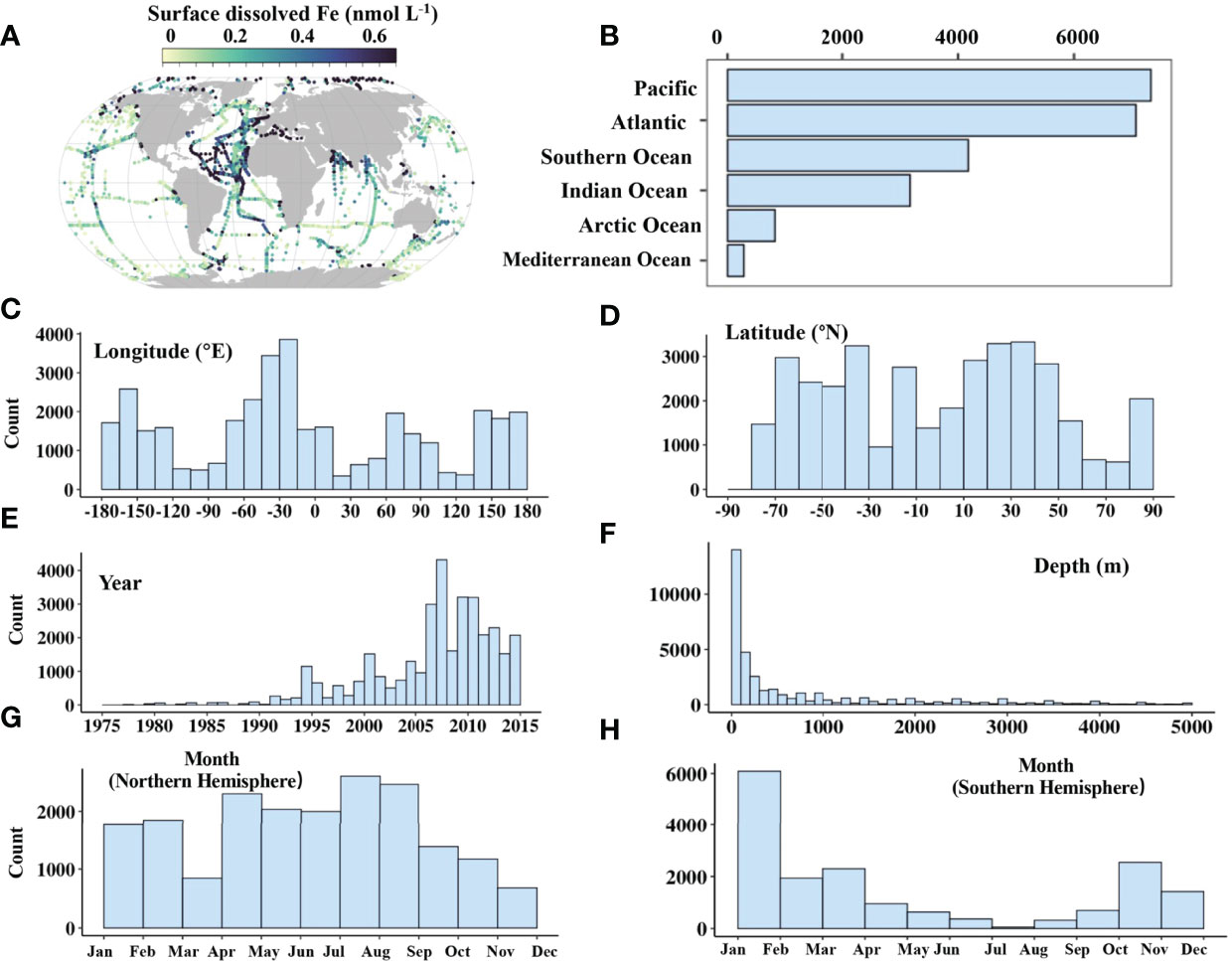
Figure 1 Distribution of compiled global observation dataset of dissolved Fe with the respect to surface ocean (A), main ocean basin (B), longitude (C), latitude (D), sampling year (E), sampling depth (F) and month (G, H). The Southern Ocean is defined as the region south of 40°S. The delineation of each ocean basin is shown in Figure S3.

2.1.2 Environmental Predictors

A suite of environmental predictors was selected, including basic sampling information (i.e., locations, sampling depth and time), physicochemical and biological parameters from contemporaneous satellite observations, reanalysis products and other model outputs. The data sources and resolution of these environmental predictors are listed in Table 1. The environmental parameters were matched with the dFe measurements according to the sampling day and location.

TABLE 1

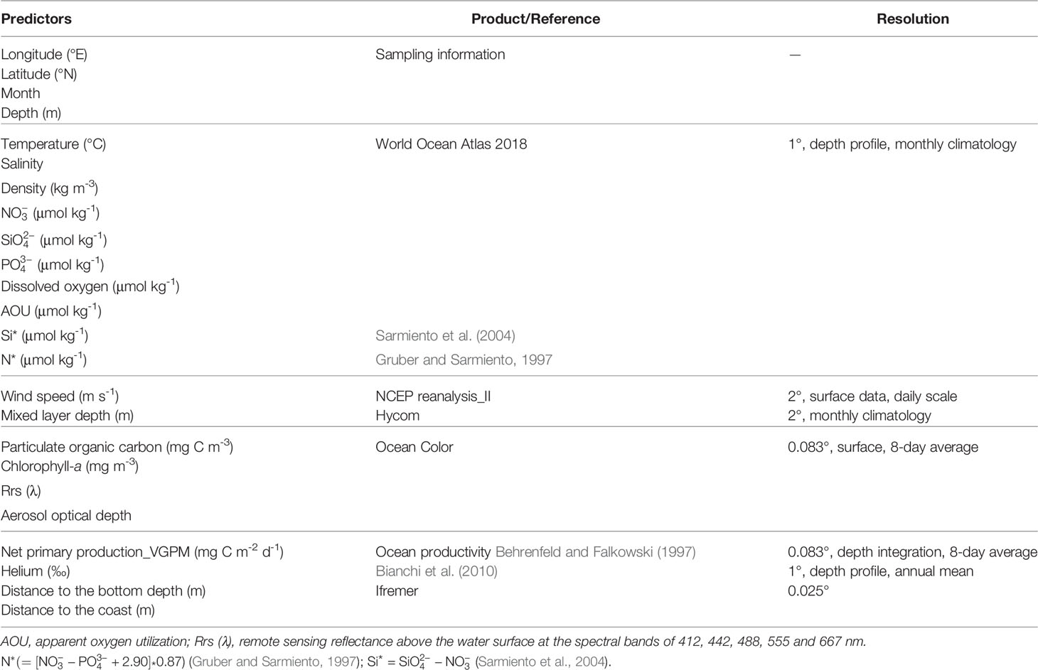
Table 1 Environmental predictors used for the model construction.

In light of our limited understanding of the intricate interplay of factors influencing dFe cycling, we intentionally include a large number of predictors and allow the statistical models to identify the most important ones. Properties such as temperature, salinity, macronutrients, dissolved oxygen concentration and composite biogeochemical tracers, such as apparent oxygen utilization (AOU), N*, and Si* (see below), link to the underlying processes that affect the distribution of dFe in the ocean (e.g., via biology and chemistry such as precipitation and scavenging by particles, complexation with organic ligands and redox transformations, large-scale ocean circulation) (Tagliabue et al., 2014c; Resing et al., 2015). AOU integrates information about water ventilation, remineralization, water age and ocean circulation (Ito et al., 2004). ${\text{N}}^{*}{\text{(=[NO}}_3^{-}-{\text{PO}}_4^{3-}+2.90]*0.87)$ represents the distribution of denitrification and N₂ fixation in the global ocean (Gruber and Sarmiento, 1997). The process of N₂ fixation may be linked to dFe distribution because of its high demand for Fe (Kustka et al., 2002; Dutkiewicz et al., 2012). Si*, defined as ${\text{Si}}^{*}={\text{SiO}}_4^{2-}-{\text{NO}}_3^{-}$, traces the transport of the iron-limited subantarctic mode waters to the subantarctic front and impacts surface plankton communities (Sarmiento et al., 2004).

Wind speed and mixed layer depth provide some insight into the role of surface forcing and the strength of vertical mixing in driving dFe patterns (Tagliabue et al., 2014b). Because dFe is a micronutrient, biological properties partly reflect their dFe status. Therefore, we included a wide spectrum of remotely-sensed biological metrics such as chlorophyll-a, particulate organic carbon (a proxy of biomass), and net primary production (Behrenfeld and Falkowski, 1997). Optical properties (Rrs) were also included because they provide some information about plankton community characteristics (Li et al., 2013). Given the importance of Fe sources from aeolian (Conway and John, 2014; Cassar et al., 2007; Hamilton et al., 2020; Tang et al., 2021), hydrothermal (Tagliabue et al., 2010; Resing et al., 2015; Roshan et al., 2020), coastal, riverine and benthic inputs in some regions (Elrod et al., 2004; Lam and Bishop, 2008), we also incorporated satellite estimates of the aerosol optical depth, model-simulated helium concentration (Bianchi et al., 2010), and distance to the coast and from the seafloor.

2.2 Data-Driven Model Construction and Validation

2.2.1 Data Processing

The overall workflow for the data processing, model construction and statistical analyses is illustrated in Figure 2. To avoid spatial autocorrelation and the overfitting induced by using near-neighbor values, measured dFe data and paired environmental parameters were gridded onto 1° × 1° horizontal grid with 31 vertical levels following the PISCES model [Aumont et al. (2015)]: 5, 15, 25, 35, 45, 55, 65, 75, 85, 95, 106, 117, 129, 142, 159, 181, 216, 271, 362, 508, 730, 1030, 1404, 1830, 2289, 2768, 3257, 3752, 4250, 4750, 5250 m. The sampling coordinates (longitude and latitude) and months were converted to periodic functions using sine and cosinece data (Eq. 1-Eq. 2) (Gade, 2010):

$\begin{array}{ll}Coordinates=\left[sin\left(lattiude \frac{\pi }{180}\right),sin\left(longitude \frac{\pi }{18}\right)cos\left(latitude \frac{\pi }{18}\right),\mathrm{co}s\left(longitude \frac{\pi }{10}\right)cos\left(latitude \frac{\pi }{180}\right)\right]& \text{Eq. 1}\end{array}$

FIGURE 2

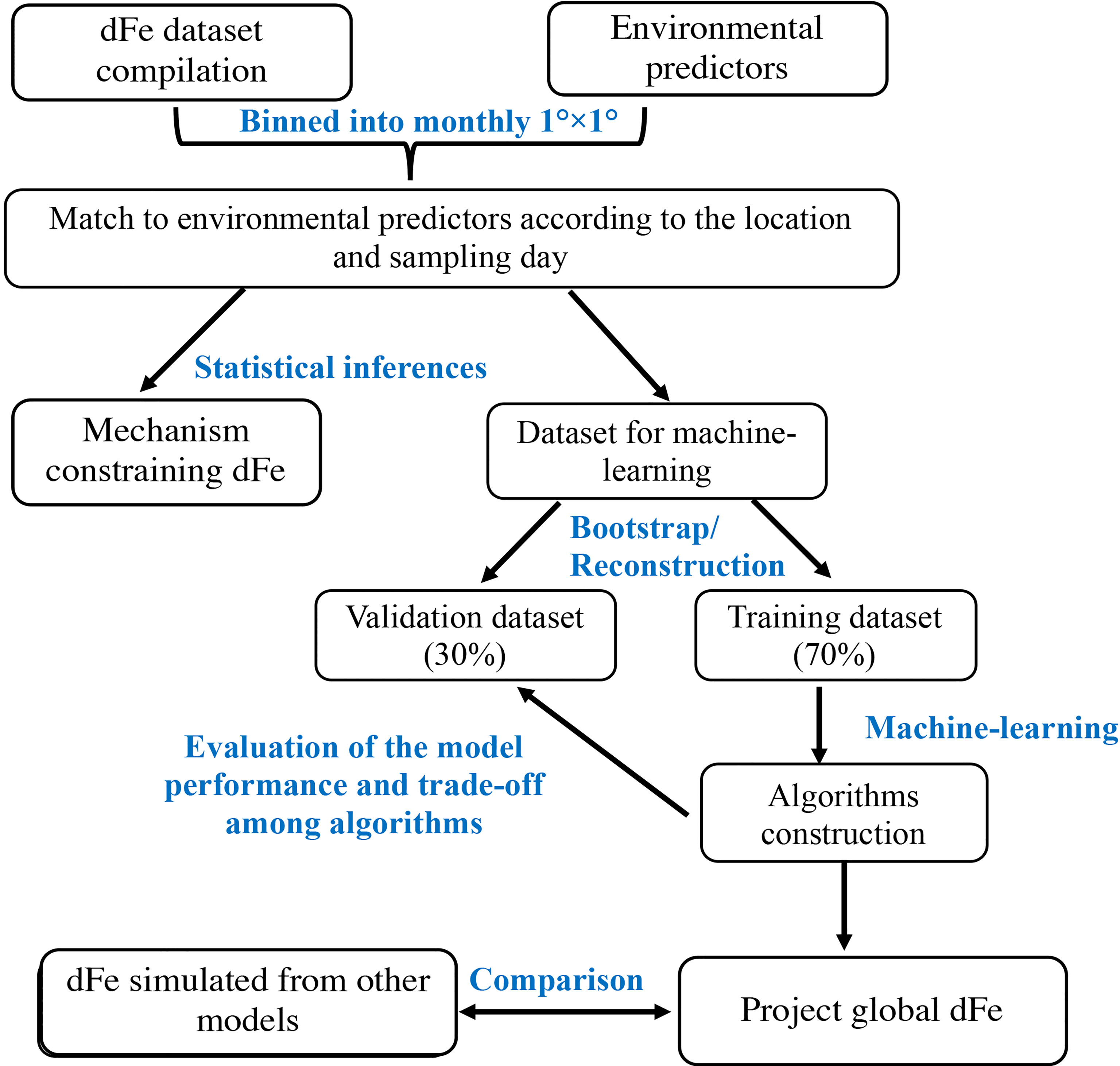
Figure 2 Workflow for the data processing, model construction and statistical analyses.

$\begin{array}{ll}Time=\left[cos\left(month \frac{2\pi }{12}\right), sin\left(month \frac{2\pi }{12}\right)\right]& \text{Eq. 2}\end{array}$

All the data were log-transformed to ensure a normal distribution.

2.2.2 Model Construction and Validation

The processed dataset was randomly divided into training (70 %) and validation datasets (30 %). For training, we used the ML techniques of random forest (RF), super vector machining (SVM), and artificial neural network (ANN). While the three techniques differ in how they find the optimal predictand solution from predictors, their general objective is to minimize the error between the observed and predicted dFe.

Briefly, RF is an ensemble algorithm composed of multiple individual decision trees which are constructed by a bootstrap sampling of the training dataset (Liaw and Wiener, 2002). Each individual tree splits out a class prediction and the class with the most votes become the model’s prediction. RF was implemented using the function ‘randomForest’ in the R package ‘randomForest’. The number of decision trees and minimum leaf size in our study were set to 300 and 20, respectively. SVM is a supervised learning model that searches for the hyperplane from the observations used for the classification or regression (Noble, 2006). SVM was performed using the function ‘svm’ in the R package ‘e1071’. The Kernel used in training and predicting is set to radial basis, with epsilon, gamma and the cost of constraints violation set to 0.2, 0.1, and 3, respectively. ANN is a nonlinear system using hyperbolic tangent as its activation function between the input and hidden layer (Wu and Feng, 2018). To reduce the dynamic range (Rafter et al., 2019; Wang et al., 2020), the dataset used to train the ANN was further standardized to their z-scores using Gaussian kernel $(\text{Z}=(\text{C}-\overline{C})/\sigma$ where C, $\overline{C}$ and σ represent the predictor’s individual concentration, mean concentration and standard deviation, respectively). ANN was trained using the R package ‘keras’. The architecture of our ANN consists of one input layer with node numbers equivalent to the number of environmental predictors (n=26), two hidden layers with nodes of 50 for both, and an output layer with a single node corresponding to the predicted dFe (n=1). The epoch, activation function and learning rate were set to 300, ‘rlu”, and 0.001, respectively. The optimizer of “Adam” was adopted to fit the model. In order to assess the added-value of using ML to model the complex distribution of dFe in the ocean, we compared the accuracy of our predictions to the more traditional statistical approach of multiple linear regression (MLR). The MLR was implemented using the function ‘lm’ in the R package ‘stats’.

The model performance was evaluated using the regression coefficients (R²) and root mean standard errors (RMSE) between predicted dFe and observed dFe from the validation dataset. To further assess the robustness of our predictions and dependence on the training dataset, we used a bootstrap approach to repeatedly reconstruct the training dataset and then calculated the coefficient of variation of the predicted dFe from 1000 iterations (c.v.= standard deviation/mean × 100 %). An attempt to build a data-driven algorithms for specific depth ranges (0-200 m, 200-1000 m, 1000-2500 m and >2500 m) did not improve the model accuracy compared to ML trained on the entire dataset (Figure S1). Finally, we used the RF algorithm (given its better performance, see section 3.2) to map the global climatology of dFe with a 1°×1° resolution at 31 vertical intervals as aforementioned.

2.3 Insight Into Mechanisms Governing dFe

We adopted two approaches to identify factors potentially influencing the spatial and temporal variability of dFe. First, we calculated the Pearson correlation coefficient between the field collected dFe samples and environmental predictors. Second, we sought the most important factors in predicting dFe concentrations by extracting the predictors that persistently ranked in the top three in relative importance during the repeated reconstruction of the training dataset used in the RF algorithm development. We applied these two statistical inferences in the subsets of the multiple depth intervals. We also derived the ferricline depth by extrapolating our data-driven predictions to profiles with 1m resolution. The ferricline is defined as the depth with the steepest vertical gradient in dFe Tagliabue et al. (2014b).

2.4 Comparison With dFe From Process-Based Models

We used our global dFe climatology as a reference to compare the performance of 13 ocean biogeochemistry models (OBM) compiled by Tagliabue et al. (2016a). Some of these OBMs have been used to specifically study global patterns of dFe cycling, and others have more broadly been used to simulate coupled climate-carbon systems as part of the recent Intergovernmental Panel on Climate Change (IPCC) report for studies. The OBM features and settings are summarized in Table 1 of Tagliabue et al. (2016a). For our comparisons, the dFe simulations from the OBM were temporally and spatially matched to our global Fe projections. While we use data-driven climatology as a reference in this study, we note that statistical models, just like process-driven models, have drawbacks and carry uncertainties, as discussed in section 3.5.

3 Results and Discussion

3.1 Global Distribution of Observational dFe Dataset

The global compilation dataset consists of over 32,000 measured dFe at the discrete depth intervals, covering the main ocean domains, and longitude and latitude bands (Figure 1). The Pacific and the Atlantic Ocean encompass the most dFe measurements among the basins, partly due to their large area (Figure 1B). The number of dFe measurements increase from around 1995 (Figure 1E) and with the start of the GEOTRACES program in 2010 (Anderson and Henderson, 2005). 70 % of samples were collected in the upper 500 m (Figure 1F). Compared to the relatively homogenous distribution of sampling months in the northern hemisphere, the striking feature in the southern hemisphere is the scarce number of measurements in the austral winter (Figures 1G, H).

3.2 Model Performance

The algorithms trained by ML approach outperform conventional linear regressions as reflected by the R² and RMSE (~0.8 vs. 0.5 and ~0.5 vs. 0.3 nmol L^-1, respectively, Figure 3). RF tends to overestimate in the lower range and underestimate in the higher range of dFe concentrations (Figure 3B). The SVM and ANN appear to do a better job in predicting endmembers, results in more scatter than the RF algorithm relative to observations (Figures 3C–E). All ML-based projections display larger errors at shallower depths and none of the models show stronger predictive skills at specific depth intervals (Figure 3F). The c.v. of the projected dFe from the data-driven model obtained from 1000 repeated reconstructions of the training dataset using a bootstrap approach (Figure 4) suggests that the RF algorithm was less sensitive to the selection of the training dataset (generally less than 20 %). The higher c.v. of SVM and ANN suggests that they may not be as stable (Figure 4). Hereafter, we focus our analyses on the global dFe climatology obtained using the RF algorithm given its greater stability with respect to the training dataset and the capability to rank the features importance.

FIGURE 3

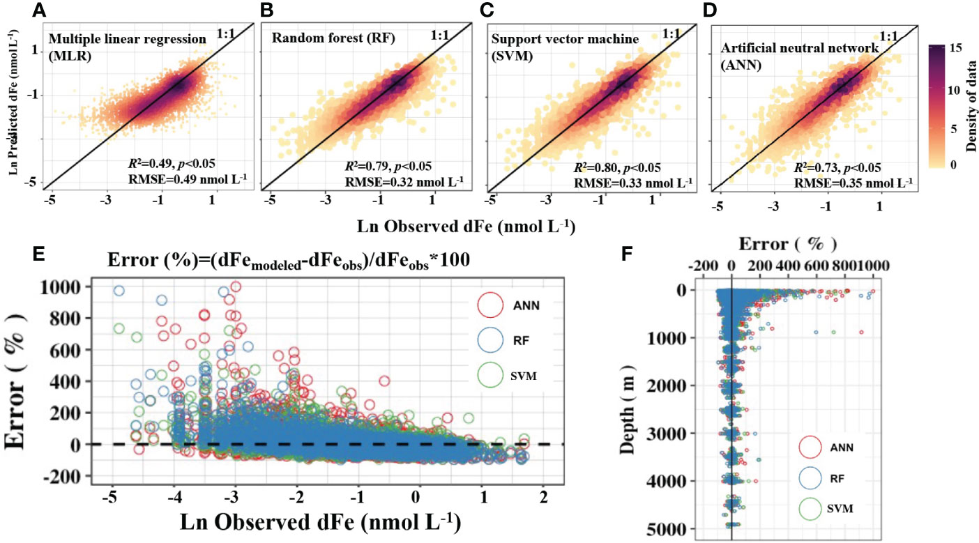
Figure 3 Model performance evaluated with the validation dataset. (A–D) show model accuracy for the different algorithms; (E, F) display the model errors alongside the magnitude of dissolved Fe (dFe) and sampling depth. RMSE, root mean standard error.

FIGURE 4

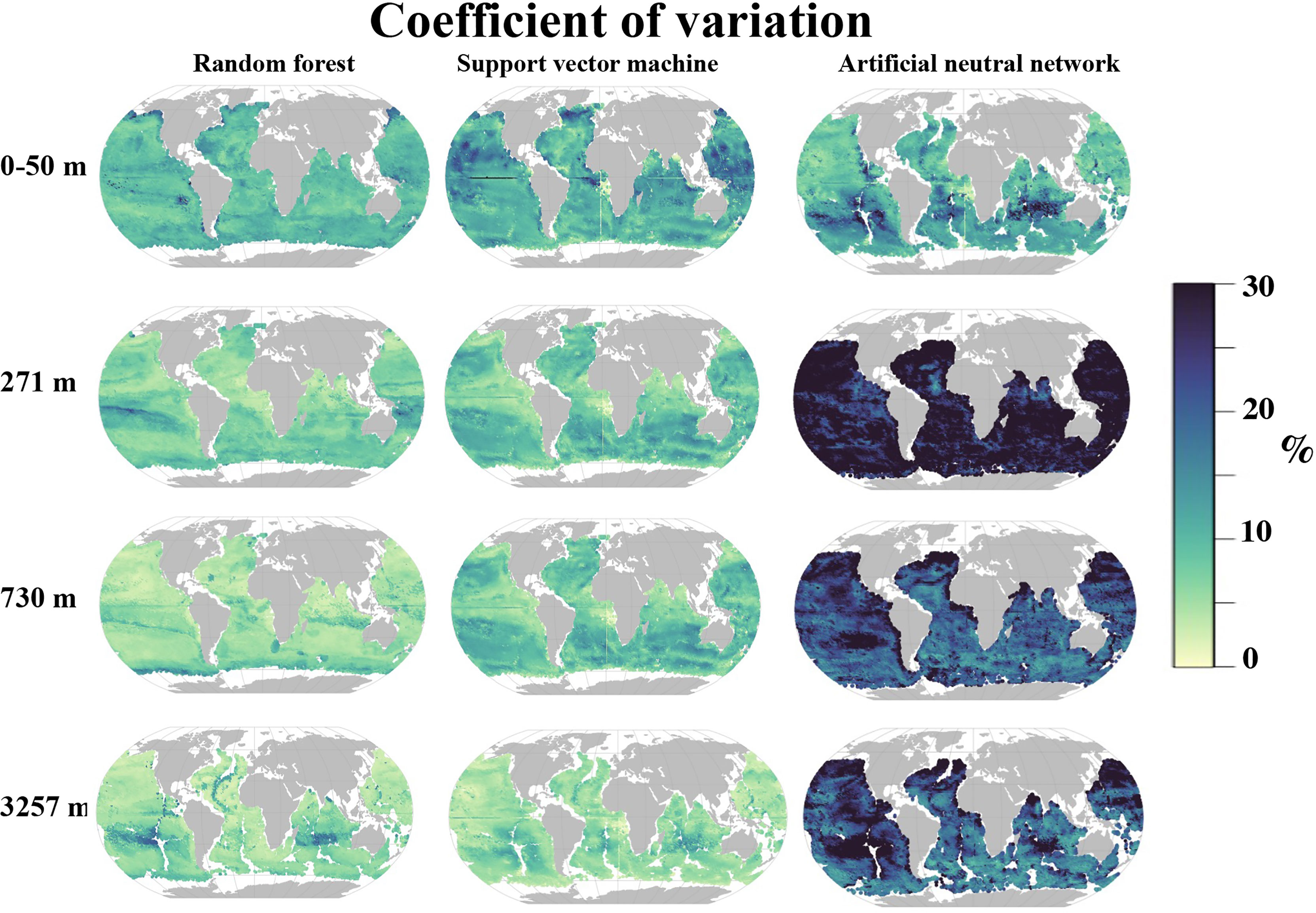
Figure 4 Coefficient of variation of projected dissolved Fe calculated from 1000 reconstruction of the training dataset using three machine-learning algorithms.

3.3 Global Climatology of Projected dFe and Potential Underlying Mechanism

The new global scale estimates of dFe achieved from our data-driven model can be used to advance our understanding of the regional magnitude and temporal dynamics of dFe in the contemporary ocean. Furthermore, the global patterns of dFe climatology and predictors provide an opportunity to assess the underlying mechanisms potentially governing the global dFe distribution at various depth horizons.

3.3.1 Surface Layer

dFe is a limiting nutrient in many regions of the surface ocean (Martin, 1990; Tagliabue et al., 2017). As expected, our data-driven model projects a prevalence of low surface dFe concentrations in many regions of the world ocean (typically less than 0.3 nmol L^-1, Figures 5A–C). Elevated surface dFe concentrations are found in the low latitude regions of the Arabian Sea, tropical Atlantic and continental margins, consistent with prior studies (Johnson et al., 1997; Rijkenberg et al., 2014).

FIGURE 5

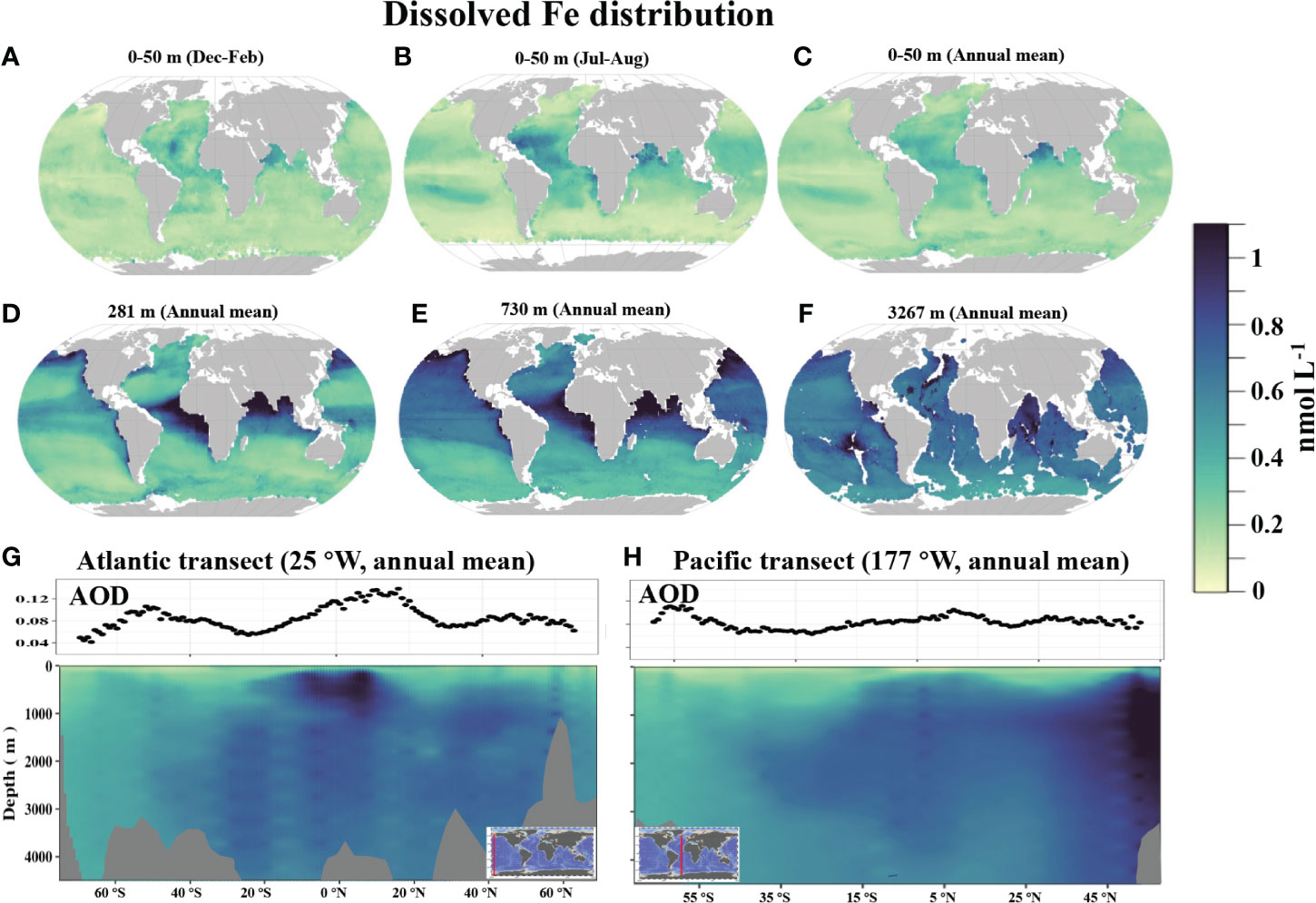
Figure 5 The global modeled dissolved Fe using the random forest approach. (A–F) show global maps of modeled dissolved Fe at various depth horizons; (G, H) display the corresponding dissolved Fe transects across the Atlantic and Pacific.

In the upper ocean, our analysis suggests that remotely-sensed aerosol optical depth is the best predictor of dFe (r=0.37, p<0.05, Table 2), with elevated surface dFe coinciding with high aerosol optical depth (Figures 5A–C and 6A, B). The pattern also holds for the seasonal cycle of both properties with surface dFe varying seasonally by a factor of two or more. The relation of surface dFe and aerosol optical depth supports the important role of aeolian dust in regulating the spatial and temporal variability in dFe concentrations in the tropical ocean (Johnson et al., 1997; Hamilton et al., 2020; Conway and John, 2014), with the caveat that remotely sensed AOD does not necessarily directly translate into aerosol deposition.

TABLE 2

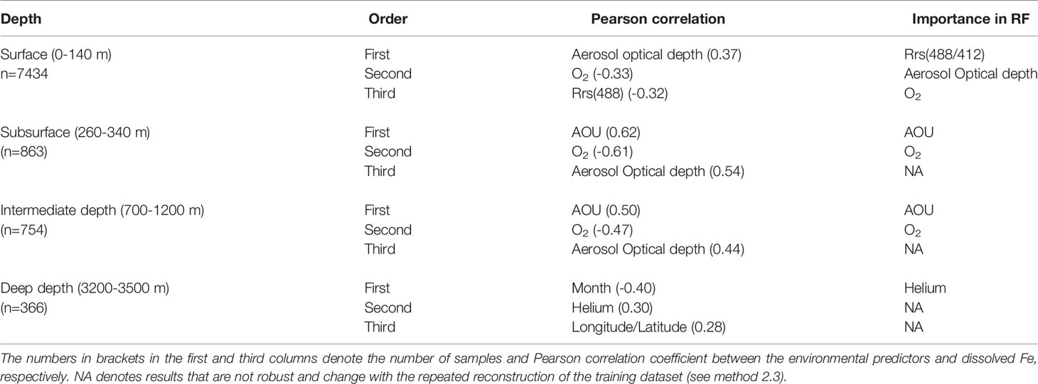
Table 2 Most important environmental predictors based on Pearson correlation and importance in the construction of the random forest (RF) algorithm (only top three are shown; the comprehensive results for all the predictors are provided in Table S1 and Figure S2).

FIGURE 6

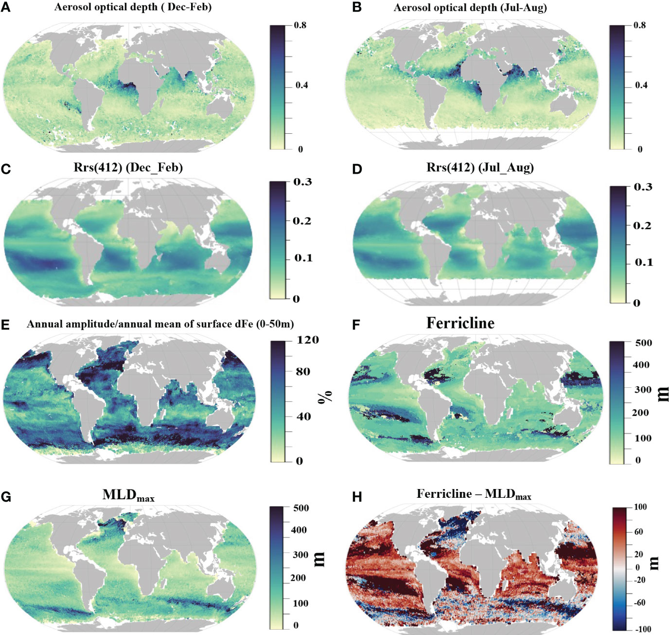
Figure 6 Global distributions of remotely-sensed aerosol optical depth (A, B), surface optical reflectance,Rrs(412) (C, D), seasonal variability of dissolved Fe represented as the percentage of the annual variance relative to the annual mean, (E) ferricline depth, (F), annual deepest mixed layer (MLD_max) (G) and the difference in ferricline and MLD_max (H).

The correlation of dissolved oxygen concentration with surface dFe is as high as for aerosol optical depth but negative (r=-0.33, p<0.05, Table 2). This negative correlation likely is not causal, and more likely results from low dFe generally being observed in the high latitudes, where O₂ solubility is high because of the cold water temperatures (Garcia and Gordon, 1992). In addition, satellite-retrieved surface ocean reflectance [i.e., Rrs(448/412)] is identified as an important feature in RF model construction (r=-0.32, p<0.05, Table 2). Water reflectance is impacted by intrinsic water properties, community structure, dissolved organic matter and detritus (Li et al., 2013; Dutkiewicz et al., 2019). The elevated surface dFe in the ultra-oligotrophic South Pacific Gyre align with the higher Rrs(412) signal (Figures 6C, D). It is unclear if the elevated dFe reflects accumulation of surface dFe due to the unique ecological characteristics of the region [weak biological activity under ultra-oligotrophic conditions, Yang et al. (2019); Quay et al. (2020)], or alternatively if it can be attributed to the misrepresentation of dFe in our data-driven model due to the limited number of observations in this region.

Another feature in the surface projection worth pointing out is that our model exhibited a higher surface dFe during summertime as opposed to winter in the Southern Ocean [as noted in prior compilations, Tagliabue et al. (2012)], which appears to contrast with a common axiom that active biological drawdown of dFe in the growing season (austral summer) and subsequent enrichment of dFe via the winter mixing. Combined with some high summer dFe (probably collected from regions with higher iron due to the island mass effect, e.g., Kerguelen and Crozet plateau), the uneven distribution of the training data is likely responsible for distorting the seasonal pattern of dFe in the Southern Ocean.

3.3.2 Subsurface and Intermediate Layers

In the subsurface layer (here shown as 271 m in Figure 5D), high dFe are observed in the tropics and subpolar Pacific. At this depth horizon, AOU emerges as the top predictor of dFe distribution as demonstrated by the Pearson correlation coefficient to individual field dFe observations (r=0.62, p<0.05, Table 2) and the spatial patterns (Figures 5D and 7A). The relationship between deep dFe and AOU has been documented in previous studies (Martin and Michael Gordon, 1988; Tagliabue et al., 2010; Tagliabue et al., 2019). AOU reflects local remineralization and spatiotemporally accumulated oxygen consumption due to the ocean circulation, with the latter tending to be predominant in the deeper layer (Ito et al., 2004). The correlation between dFe and AOU is known to be confounded by the removal of remineralized dFe via scavenging as reflected by observed Fe:O ratios diverging from those expected from sinking particulate material (Tagliabue et al., 2019). The generally elevated subsurface dFe in equatorial and high latitude regions is a result of mesopelagic respiration fueled by upper layer organic matter export in these productive regions. In addition, the upwelling in the equatorial Pacific (Wyrtki, 1981) can bring deep dFe to the subsurface depth. The highest subsurface AOU and dFe are found in the Arabian Sea and southeast tropical Pacific (Figures 5D and 7A), which are well-known oxygen minimum zones (OMZs). The mesopelagic respiration occurring at OMZs (Tiano et al., 2014), potentially coupled with reduced scavenging and oxidation of dFe under low oxygen condition (Tagliabue et al., 2019), may thus drive the high dFe in these regions.

FIGURE 7

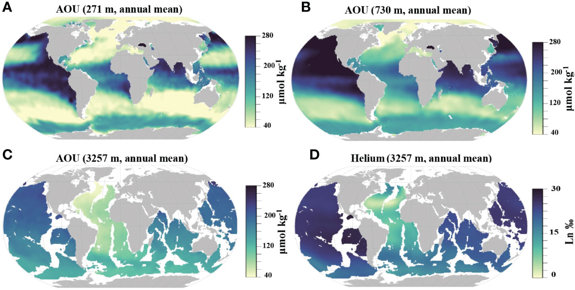
Figure 7 Global distribution of apparent oxygen utilization (AOU) at 271 m (A), 730 m (B), 3257m (C), and helium concentration at 3257 m (D).

In addition to AOU, the aerosol optical depth also shows a high correlation with the observed subsurface dFe (r=0.54, p<0.05, Table 2). From vertical distributions in the Pacific and Atlantic (Figures 5G, H), and mean profiles (Figure 8), we observe high dFe penetrating deeper in the water column (up to 2000-3000 m) in these dust-impacted regions. Studies have shown that Fe-rich dust can impact the entire column (Bruland et al., 1994; Johnson et al., 1997) via a range of processes such as dissolution of aeolian iron, enhanced mesopelagic remineralization through an increase in particle flux from the surface ocean thereby altering the deep organic complexing-ligands (Wozniak et al., 2015) or not being consumed by phytoplankton in the upper layer due to other nutrients being limiting (Bruland et al., 1994; Wu and Luther, 1994). In the subtropical gyres of the North Atlantic, higher dFe concentrations at the subsurface than in overlaying waters is perhaps driven by equatorward subduction and transport of excess dFe and organic Fe ligands from the more northern latitudes (Tagliabue et al., 2019).

FIGURE 8

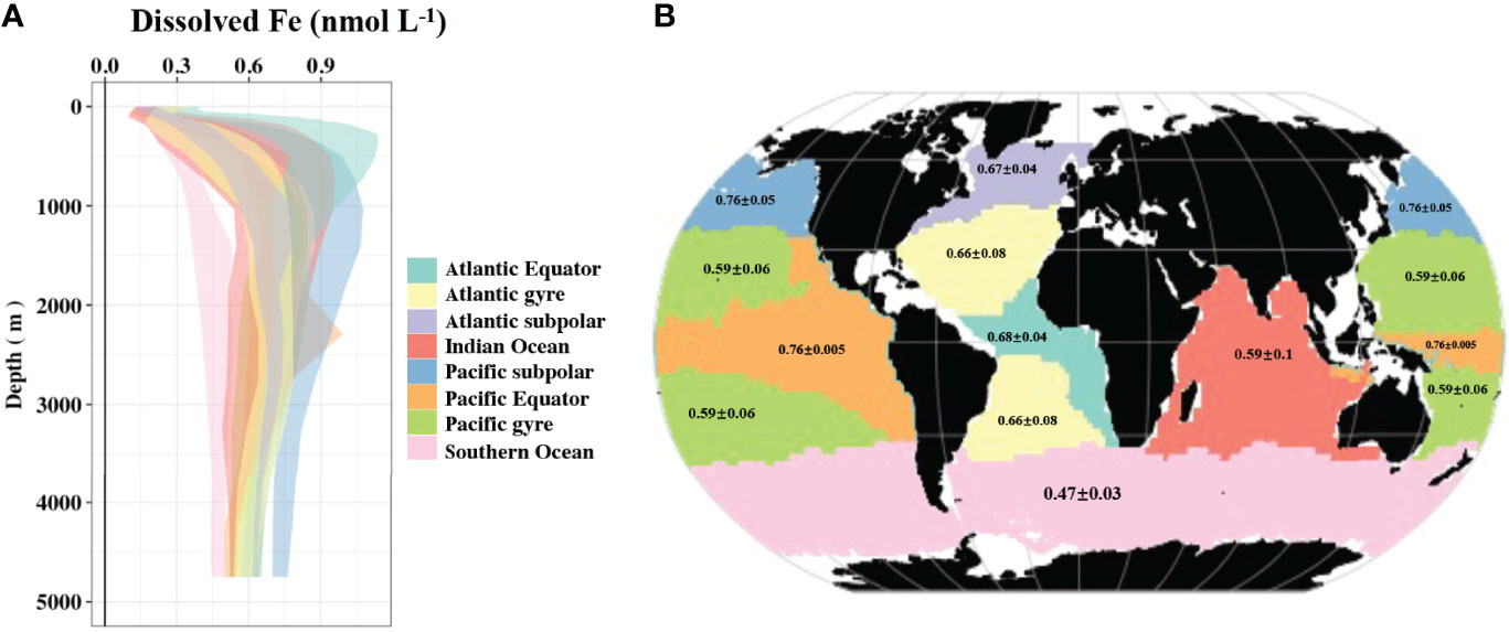
Figure 8 Mean profile of dissolved Fe (dFe) with the shading representing the standard deviation (A), and mean dFe concentration (±standard deviation) at the depth between 3000 m and 3500 m (B) in the main ocean basin.

The distribution of dFe in the subsurface also provides a qualitative insight into the potential for vertical entrainment. We compare the depth difference between annual deepest mixed layer and ferricline, which provide information about the potential of vertical dFe supply from the subsurface to the surface via the seasonal entrainment. We find that the deepest winter mixed layer depths rarely extend to the ferricline in the tropical Pacific and subpolar Pacific (Figures 6F–H). In contrast, the deep mixed layers in the subpolar Atlantic and some regions of Southern Ocean (e.g., subantarctic zone) extend to the ferricline (Figure 6). However, we note that entrainment supply of dFe is not only controlled by the ferricline depth. Entrainment input of dFe is determined by the volume of water being entrained during winter and detrainmented in the subsequent spring, together with the concentration difference of dFe between the mixed layer and underlying waters. These processes vary regionally (Rigby et al., 2020). For example, the persistently-low subsurface dFe in the subpolar Atlantic and subantarctic zone (Figure 5D) may limit the total amount of dFe that can be pumped via winter mixing even when mixing reaches the ferricline. In principle, the amount of dFe supply via vertical entrainment can be quantified by a combination of our modeled monthly dFe profile and seasonally varying mixed layer depth. Yet, we are cautious about overinterpretation of the present results because the global map of the ferricline depth obtained from our data-driven model is coarse, especially when it is diagnosed to be deeper than 200 m due to coarse resolution of vertical grids below 200 m in our projection (10 m spacing in the upper 200 m and 20-300m spacing between 200 m and 1000 m).

In the intermediate layers (here shown as 730 m in Figure 5E), AOU is still the top predictor of the dFe variability (Table 2, r=0.50, p<0.05). dFe generally increases equatorward in the southern hemisphere (Figure 5E). Water masses at these depths are generally composed of mode waters originating from the subantarctic (Herraiz-Borreguero and Rintoul, 2011). The increasing dFe likely reflects an accumulated remineralization signal along the Subantarctic Mode Water and Antarctic Intermediate Water pathways, reinforced by similar trends in AOU (Table 2 and Figure 7C) (Tagliabue et al., 2019).

3.3.3 Deep Layer

The variability of dFe at depth is relatively small, ranging from 0.4-0.7 nmol L^-1 (Figures 5E, 8). This has been hypothesized to result from relatively uniform concentrations of organic iron-complexing ligands in the ocean interior that act as a buffer on dFe concentrations (Gledhill and van den Berg, 1994; Johnson et al., 1997), although recent studies reveal more spatial heterogeneity than previously thought (Tagliabue et al., 2014c; Buck et al., 2015; Gerringa et al., 2015a). Despite the small variability, the deep layer still displays some distinct features, with the highest dFe in the subpolar and equatorial Pacific and the lowest dFe in the Southern Ocean. As the end of the overturning circulation, the subpolar Pacific preserves the footprint of dFe signals accumulated alongside the circulation. The Southern Ocean receives the lowest input of aeolian and sedimentary dFe (Hamilton et al., 2020). Moreover, due to the high levels of major nutrients, dFe is often strongly depleted by the end of the upper ocean growing season. Deep water masses, like Antarctic Bottom Water, form in the region and transport these low dFe values to the ocean interior. These younger water masses have had little chance to accumulate additional dFe from regeneration and hence deep water dFe values are the lowest in the global ocean. The lowest dFe observed in the Southern Ocean is aligned with the lowest δ¹⁵N found in the abyssal Southern Ocean among global ocean basin, suggesting a correlation to remineralization (Rafter et al., 2019). Such a pattern is also confirmed by the relatively low amount of sinking particles exported to depth in the Southern Ocean as estimated from sediment trap observations and satellite-based models (Elrod et al., 2004; Lam et al., 2008).

In line with a number of recent studies showing the importance of hydrothermal dFe sources along mid-ocean ridges (Tagliabue et al., 2010; Tagliabue et al., 2014a; Resing et al., 2015; Roshan et al., 2020), helium concentration, a tracer of hydrothermal activity, ranked as one of the important predictors for deep dFe distribution (r=0.30, p<0.05, Table 2). However, no consistent pattern was observed between the global distribution of helium and projected dFe at depth (Figures 5F and 7D). This is probably due to the different water column chemistry that decouples Fe from helium (Tagliabue and Resing, 2016b), as well as the impact of other local iron sources, such as sedimentary input (Elrod et al., 2004; Lam et al., 2008). Additionally, some patches of dFe emerge in the Northern Atlantic and South Pacific Gyre (Figure 5F). These patches are in regions with high bootstrap c.v. (Figure 4), implying that the dFe predictions in these regions are sensitive to the selection of the training dataset and therefore may not be robust.

3.4 Comparison With Process Model Simulations

We assess the OBM performance using our reference climatology from our data-driven model, building upon the previous effort of Tagliabue et al. (2016a) who used discrete observations. In the upper 200 m, while the correlation of dFe between the thirteen process-based models versus the data-driven model converge to 0.4, the RMSE vary widely from 0.15 to 0.5 nmol L^-1 (Figure 9A). This implies consistency in relative variability in dFe distribution at the surface but some differences in the absolute magnitude of dFe. Tagliabue et al. (2016a) found that most OBM reproduced the predicted enhancement in surface dFe in the tropical Atlantic, Arabian Sea and continental margins, but that some models’ representation of surface sources and biological uptake resulted in varying surface dFe concentrations. At depth, the OBMs skills were more variable, with Pearson correlation coefficients ranging from -0.4 to 0.6 (Figures 9B–D), depending on whether the models include or properly represent important Fe cycling processes occurring in the deep ocean, including organic blinding ligand, hydrothermal vents and scavenging (Gledhill and Buck, 2012; Tagliabue et al., 2016a; Tagliabue et al., 2010). Even OBM models with high Pearson correlation coefficients (up to 0.6) tend to underrepresent the degree of spatial variability in dFe concentration at depth (Figure 9D).

FIGURE 9

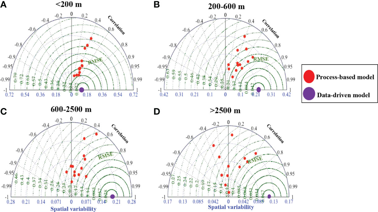
Figure 9 Taylor diagrams comparing global modeled dissolved Fe from thirteen existing process-based models against the random forest data-driven model at the depth different depth intervals (A–D). The models simulated dFe spatial variability, Pearson correlation coefficients and RMSE between process-based and the data-driven models are shown on the blue, black and green axes, respectively.

3.5 Caveats and Limitations

Our study carries limitations and caveats that need to be considered. First, biases may be present in the dFe dataset due to differences in sampling protocols and analytical techniques (Achterberg et al., 2001; Johnson et al., 2007), particularly for data collected before the implementation of the GEOTRACES program. For example, the filter pore size used as a cut-off for the dissolved phase differs between some historical studies, ranging from 0.2-0.45 um (Tagliabue et al., 2012).

Second, despite substantial progress in observations, the coverage of our training observational dataset remains uneven. For example, the winter season in the Southern hemisphere remains undersampled (Figure 1H). Extrapolation of projections from the data-driven model to under-represented regions or periods may be of acceptable quality if the algorithm captures the full range of relationships between predictors and predictants. However, because the factors regulating dFe differ among ocean regimes and timescales (Tagliabue et al., 2014a), our ML may not capture the full range of predictor-predictant relationships, and may as importantly not include some important predictors (e.g., properties important to dFe distribution not observable from space). The low c.v. obtained from repeated reconstructions of the training dataset using the bootstrap approach (Figure 4A) suggests that our results are relatively insensitive to the dataset selected used for training the algorithms, and that the subset of the entire data covers variability in the functional relationships between predictors and predictant dFe. However, the performance of our data-driven model is expected to improve as the number of observations grows.

Third, the environmental properties used as predictors also carry uncertainties. Because concurrent field measurements of environmental parameters are limited, we were forced to rely on reanalysis products (i.e., World Ocean Dataset 2018 or NCEP reanalysis-II), satellite observations and other model outputs. Some of these estimates carry substantial intrinsic uncertainties and errors associated with temporal and spatial mismatch to paired dFe observations. The ML approach may provide accurate projections if uncertainties in the predictors are systematic biases that can be captured by the algorithm. However, such biases would misrepresent the true relation between environmental factors and dFe and the mechanisms governing dFe cycling. Finally, as with more traditional statistical approaches, because the information provided by such analyses is inferential, conclusions about potential causation should be interpreted with caution and require field campaigns to further look into these patterns and underlying mechanisms. For example, our model yielded a unique vertical structure of dFe in the data-poor tropical eastern Pacific, with low surface dFe, but elevated dFe a few hundred meters beneath the surface. The relation between dFe and remotely sensed reflectance in the utra-oligotrophic South Pacific Gyre is another intriguing result that merits further exploration regarding the potential underlying mechanisms.

4 Conclusion

By leveraging a compilation of published data and a novel ML approach, we derived a global dFe climatology and explored possible mechanisms governing the dFe distribution using statistical inferences. Our study emphasizes the importance of dust input in enriching the dFe inventory at low latitudes. The correlation between AOU and dFe highlights the role of net regeneration and large-scale ocean circulation pathways as key mediators of the global dFe distribution at depth. Finally, we present a general assessment of existing OBMs using our data-driven model as reference. The uneven geographic distribution of observational dataset and uncertainty in environmental predictors remain important caveats for data-driven climatological maps. Further expansion in dFe observations together with parallel measurements of comprehensive environmental parameters, as conducted in the ongoing GEOTRACES program, will improve model simulations. While our approach carries uncertainties, our next data-based climatology may provide an independent mean to assess, evaluate, and ultimately improve the new generation of ocean iron models.

Data Availability Statement

The original contributions presented in the study are included in the article/Supplementary Material, further inquiries can be directed to the corresponding author. The products of the monthly climatological dissolved Fe generated in this study are available on the public data library Zenodo (https://zenodo.org/record/6385044#.Yn2AdBPMJhF, doi: 10.5281/zenodo.6385044) or on request to the corresponding author (nicolas.cassar.@duke.edu).

Author Contributions

NC and AT conceived and designed the project. AT compiled the dataset. YH and NC constructed the models, did the data analysis, and wrote the first draft of the manuscript, and all co-authors contributed the input to the final version. All authors contributed to the article and approved the submitted version.

Funding

NC was supported by the “Laboratoire d’Excellence” LabexMER (ANR-10-LABX-19) and co-funded by a grant from the French government under the program “Investissements d’Avenir”. AT has received funding from the European Research Council (ERC) under the European Union's Horizon 2020 research and innovation program (grant agreement no. 724289). YH was supported by Chinese State Scholarship Fund to study at Duke University as a joint Ph. D student (No. 201806310052). The work of WG 151 presented in this article results, in part, from funding provided by national committees of the Scientific Committee on Oceanic Research (SCOR) and from a grant to SCOR from the U.S. National Science Foundation (OCE-1840868).

Conflict of Interest

The authors declare that the research was conducted in the absence of any commercial or financial relationships that could be construed as a potential conflict of interest.

Publisher’s Note

All claims expressed in this article are solely those of the authors and do not necessarily represent those of their affiliated organizations, or those of the publisher, the editors and the reviewers. Any product that may be evaluated in this article, or claim that may be made by its manufacturer, is not guaranteed or endorsed by the publisher.

Acknowledgments

We are grateful to all the prior efforts in collecting, measuring and compiling dissolved iron in the global ocean and making these data publicly available, which forms the key basis for the construction of our data-driven model.

Supplementary Material

The Supplementary Material for this article can be found online at: https://www.frontiersin.org/articles/10.3389/fmars.2022.837183/full#supplementary-material

References

Achterberg E. P., Holland T. W., Bowie A. R., Mantoura R. F. C., Worsfold P. J. (2001). Determination of Iron in Seawater. Anal. Chim. Acta 442, 1–14. doi: 10.1016/S0003-2670(01)01091-1

CrossRef Full Text | Google Scholar

Anderson R., Henderson G. (2005). Program Update | GEOTRACES—A Global Study of the Marine Biogeochemical Cycles of Trace Elements and Their Isotopes. Oceanography 18, 76–79. doi: 10.5670/oceanog.2005.31

CrossRef Full Text | Google Scholar

Aumont O., Ethé C., Tagliabue A., Bopp L., Gehlen M. (2015). PISCES-V2: An Ocean Biogeochemical Model for Carbon and Ecosystem Studies. Geosci. Model Dev. 8, 2465–2513. doi: 10.5194/gmd-8-2465-2015

CrossRef Full Text | Google Scholar

Behrenfeld M. J., Falkowski P. G. (1997). Photosynthetic Rates Derived From Satellite-Based Chlorophyll Concentration. Limnol. Oceanog. 42, 1–20. doi: 10.4319/lo.1997.42.1.0001

CrossRef Full Text | Google Scholar

Bergquist B. A., Boyle E. A. (2006). Dissolved Iron in the Tropical and Subtropical Atlantic Ocean. Global Biogeochem. Cycle. 20, GB1015. doi: 10.1029/2005gb002505

CrossRef Full Text | Google Scholar

Bianchi D., Sarmiento J. L., Gnanadesikan A., Key R. M., Schlosser P., Newton R. (2010). Low Helium Flux From the Mantle Inferred From Simulations of Oceanic Helium Isotope Data. Earth Planet. Sci. Lett. 297, 379–386. doi: 10.1016/j.epsl.2010.06.037

CrossRef Full Text | Google Scholar

Bopp L., Resplandy L., Orr J. C., Doney S. C., Dunne J. P., Gehlen M., et al. (2013). Multiple Stressors of Ocean Ecosystems in the 21st Century: Projections With CMIP5 Models. Biogeosciences 10, 6225–6245. doi: 10.5194/bg-10-6225-2013

CrossRef Full Text | Google Scholar

Boyd P. W., Ellwood M. J. (2010). The Biogeochemical Cycle of Iron in the Ocean. Nat. Geosci. 3, 675–682. doi: 10.1038/ngeo964

CrossRef Full Text | Google Scholar

Boyd P. W., Jickells T., Law C. S., Blain S., Boyle E. A., Buesseler K. O., et al. (2007). Mesoscale Iron Enrichment Experiments 1993-2005: Synthesis and Future Directions. Science 315, 612–617. doi: 10.1126/science.1131669

PubMed Abstract | CrossRef Full Text | Google Scholar

Bruland K. W., Orians K. J., Cowen J. P. (1994). Reactive Trace Metals in the Stratified Central North Pacific. Geochi. Cosmochim. Acta 58, 3171–3182. doi: 10.1016/0016-7037(94)90044-2

CrossRef Full Text | Google Scholar

Buck K. N., Sohst B., Sedwick P. N. (2015). The Organic Complexation of Dissolved Iron Along the U.S. GEOTRACES (GA03) North Atlantic Section. Deep. Sea. Res. Part II. Top. Stud. Oceanog. 116, 152–165. doi: 10.1016/j.dsr2.2014.11.016

CrossRef Full Text | Google Scholar

Cassar N., Bender M. L., Barnett B. A., Fan S., Moxim W. J., Levy H., et al. (2007). The Southern Ocean Biological Response to Aeolian Iron Deposition. Science. 317, 1067–1070. doi: 10.1126/science.1144602

PubMed Abstract | CrossRef Full Text | Google Scholar

Chen B., Liu H., Xiao W., Wang L., Huang B. (2020). A Machine-Learning Approach to Modeling Picophytoplankton Abundances in the South China Sea. Prog. Oceanog. 189, 102456. doi: 10.1016/j.pocean.2020.102456

CrossRef Full Text | Google Scholar

Coale K. H., Johnson K. S., Fitzwater S. E., Gordon R. M., Tanner S., Chavez F. P., et al. (1996). A Massive Phytoplankton Bloom Induced by an Ecosystem-Scale Iron Fertilization Experiment in the Equatorial Pacific Ocean. Nature 383, 495–501. doi: 10.1038/383495a0

PubMed Abstract | CrossRef Full Text | Google Scholar

Conway T. M., John S. G. (2014). Quantification of Dissolved Iron Sources to the North Atlantic Ocean. Nature 511, 212–215. doi: 10.1038/nature13482

PubMed Abstract | CrossRef Full Text | Google Scholar

Dutkiewicz S., Hickman A. E., Jahn O., Henson S., Beaulieu C., Monier E. (2019). Ocean Colour Signature of Climate Change. Nat. Commun. 10, 578. doi: 10.1038/s41467-019-08457-x

PubMed Abstract | CrossRef Full Text | Google Scholar

Dutkiewicz S., Ward B., Monteiro F., Follows M. (2012). Interconnection of Nitrogen Fixers and Iron in the Pacific Ocean: Theory and Numerical Simulations. Global Biogeochem. Cycle. 26. doi: 10.1029/2011GB004039

CrossRef Full Text | Google Scholar

Elrod V. A., Berelson W. M., Coale K. H., Johnson K. S. (2004). The Flux of Iron From Continental Shelf Sediments: A Missing Source for Global Budgets. Geophys. Res. Letter. 31, n/a–n/a. doi: 10.1029/2004gl020216

CrossRef Full Text | Google Scholar

Fitzsimmons J. N., Boyle E. A. (2014). Both Soluble and Colloidal Iron Phases Control Dissolved Iron Variability in the Tropical North Atlantic Ocean. Geochi Cosmochim. Acta 125, 539–550. doi: 10.1016/j.gca.2013.10.032

CrossRef Full Text | Google Scholar

Fitzsimmons J. N., Hayes C. T., Al-Subiai S. N., Zhang R., Morton P. L., Weisend R. E., et al. (2015). Daily to Decadal Variability of Size-Fractionated Iron and Iron-Binding Ligands at the Hawaii Ocean Time-Series Station ALOHA. Geochi Cosmochim. Acta 171, 303–324. doi: 10.1016/j.gca.2015.08.012

CrossRef Full Text | Google Scholar

Fitzsimmons Jessica N., Boyle Edward A., Jenkins William J. (2014). Distal Transport of Dissolved Hydrothermal Iron in the Deep South Pacific Ocean. Proc. Natl. Acad. Sci. 111, 16654–16661. doi: 10.1073/pnas.1418778111

CrossRef Full Text | Google Scholar

Fitzsimmons J. N., Zhang R., Boyle E. A. (2013). Dissolved Iron in the Tropical North Atlantic Ocean. Mar. Chem. 154, 87–99. doi: 10.1016/j.marchem.2013.05.009

CrossRef Full Text | Google Scholar

Gade K. (2010). A non-Singular Horizontal Position Representation. J. Navigat. 63, 395–417. doi: 10.1017/S0373463309990415

CrossRef Full Text | Google Scholar

Garcia H. E., Gordon L. I. (1992). Oxygen Solubility in Seawater-Better Fitting Equations. Limnol. Oceanog. 37, 1307–1312. doi: 10.4319/lo.1992.37.6.1307

CrossRef Full Text | Google Scholar

Gerringa L. J. A., Laan P., van Dijken G. L., van Haren H., De Baar H. J. W., Arrigo K. R., et al. (2015b). Sources of Iron in the Ross Sea Polynya in Early Summer. Mar. Chem. 177, 447–459. doi: 10.1016/j.marchem.2015.06.002

CrossRef Full Text | Google Scholar

Gerringa L. J., Rijkenberg M. J., Schoemann V., Laan P., De Baar H. J. (2015a). Organic Complexation of Iron in the West Atlantic Ocean. Mar. Chem. 177, 434–446. doi: 10.1016/j.marchem.2015.04.007

CrossRef Full Text | Google Scholar

Gledhill M., Buck K. (2012). The Organic Complexation of Iron in the Marine Environment: A Review. Front. Microbiol. 3. doi: 10.3389/fmicb.2012.00069

CrossRef Full Text | Google Scholar

Gledhill M., van den Berg C. M. G. (1994). Determination of Complexation of Iron(III) With Natural Organic Complexing Ligands in Seawater Using Cathodic Stripping Voltammetry. Mar. Chem. 47, 41–54. doi: 10.1016/0304-4203(94)90012-4

CrossRef Full Text | Google Scholar

Grand M. M., Measures C. I., Hatta M., Hiscock W. T., Landing W. M., Morton P. L., et al. (2015a). Dissolved Fe and Al in the Upper 1000 M of the Eastern Indian Ocean: A High-Resolution Transect Along 95°E From the Antarctic Margin to the Bay of Bengal. Global Biogeochem. Cycle. 29, 375–396. doi: 10.1002/2014GB004920

CrossRef Full Text | Google Scholar

Grand M. M., Measures C. I., Hatta M., Morton P. L., Barrett P., Milne A., et al. (2015b). The Impact of Circulation and Dust Deposition in Controlling the Distributions of Dissolved Fe and Al in the South Indian Subtropical Gyre. Mar. Chem. 176, 110–125. doi: 10.1016/j.marchem.2015.08.002

CrossRef Full Text | Google Scholar

Gruber N., Sarmiento J. L. (1997). Global Patterns of Marine Nitrogen Fixation and Denitrification. Global Biogeochem. Cycle. 11, 235–266. doi: 10.1029/97GB00077

CrossRef Full Text | Google Scholar

Hain M. P., Sigman D. M., Haug G. H. (2010). Carbon Dioxide Effects of Antarctic Stratification, North Atlantic Intermediate Water Formation, and Subantarctic Nutrient Drawdown During the Last Ice Age: Diagnosis and Synthesis in a Geochemical Box Model. Global Biogeochem. Cycle. 24. doi: 10.1029/2010GB003790

CrossRef Full Text | Google Scholar

Hamilton D. S., Moore J. K., Arneth A., Bond T. C., Carslaw K. S., Hantson S., et al. (2020). Impact of Changes to the Atmospheric Soluble Iron Deposition Flux on Ocean Biogeochemical Cycles in the Anthropocene. Global Biogeochem. Cycle. 34, 12. doi: 10.1029/2019gb006448

CrossRef Full Text | Google Scholar

Herraiz-Borreguero L., Rintoul S. R. (2011). Subantarctic Mode Water: Distribution and Circulation. Ocean. Dynam. 61, 103–126. doi: 10.1007/s10236-010-0352-9

CrossRef Full Text | Google Scholar

Huang Y., Nicholson D., Huang B., Cassar N. (2021). Global Estimates of Marine Gross Primary Production Based on Machine Learning Upscaling of Field Observations. Global Biogeochem. Cycle. 35. doi: 10.1029/2020GB006718

CrossRef Full Text | Google Scholar

Hutchins D. A., DiTullio G. R., Zhang Y., Bruland K. W. (1998). An Iron Limitation Mosaic in the California Upwelling Regime. Limnol. Oceanog. 43, 1037–1054. doi: 10.4319/lo.1998.43.6.1037

CrossRef Full Text | Google Scholar

Ito T., Follows M. J., Boyle E. A. (2004). Is AOU a Good Measure of Respiration in the Oceans? Geophys. Res. Lett. 31, L17305. doi: 10.1029/2004gl020900

CrossRef Full Text | Google Scholar

Jaccard S. L., Galbraith E. D., Martínez-García A., Anderson R. F. (2016). Covariation of Deep Southern Ocean Oxygenation and Atmospheric CO₂ Through the Last Ice Age. Nature 530, 207–210. doi: 10.1038/nature16514

PubMed Abstract | CrossRef Full Text | Google Scholar

Johnson K. S., Elrod V., Fitzwater S., Plant J., Boyle E., Bergquist B., et al. (2007). Developing Standards for Dissolved Iron in Seawater. Eos. Trans. Am. Geophys. Union. 88, 131–132. doi: 10.1029/2007EO110003

CrossRef Full Text | Google Scholar

Johnson K. S., Gordon R. M., Coale K. H. (1997). What Controls Dissolved Iron Concentrations in the World Ocean? Mar. Chem. 57, 137–161. doi: 10.1016/S0304-4203(97)00043-1

CrossRef Full Text | Google Scholar

Kohfeld K. E., Ridgwell A. (2009). Glacial-Interglacial Variability in Atmospheric CO₂. Surf. Ocean–Low. Atmos. Process. 187 (2009), 251–286 doi: 10.1029/2008GM000845

CrossRef Full Text | Google Scholar

Kustka A., Carpenter E. J., Sañudo-Wilhelmy S. A. (2002). Iron and Marine Nitrogen Fixation: Progress and Future Directions. Res. Microbiol. 153, 255–262. doi: 10.1016/S0923-2508(02)01325-6

PubMed Abstract | CrossRef Full Text | Google Scholar

Lambert F., Tagliabue A., Shaffer G., Lamy F., Winckler G., Farias L., et al. (2015). Dust Fluxes and Iron Fertilization in Holocene and Last Glacial Maximum Climates. Geophys. Res. Lett. 42, 6014–6023. doi: 10.1002/2015gl064250

CrossRef Full Text | Google Scholar

Lam P. J., Bishop J. K. B. (2008). The Continental Margin Is a Key Source of Iron to the HNLC North Pacific Ocean. Geophys. Res. Lett. 35. doi: 10.1029/2008GL033294

PubMed Abstract | CrossRef Full Text | Google Scholar

Liaw A., Wiener M. (2002). Classification and Regression by Randomforest. R. News. 2, 18–22.

Google Scholar

Li Z., Cassar N. (2016). Satellite Estimates of Net Community Production Based on O₂/Ar Observations and Comparison to Other Estimates. Global Biogeochem. Cycle. 30, 735–752. doi: 10.1002/2015GB005314

CrossRef Full Text | Google Scholar

Li Z., Li L., Song K., Cassar N. (2013). Estimation of Phytoplankton Size Fractions Based on Spectral Features of Remote Sensing Ocean Color Data. J. Geophys. Res.: Ocean. 118, 1445–1458. doi: 10.1002/jgrc.20137

CrossRef Full Text | Google Scholar

Marchetti A. (2019). A Global Perspective on Iron and Plankton Through the Tara Oceans Lens. Global Biogeochem. Cycle. 33, 239–242. doi: 10.1029/2019gb006181

CrossRef Full Text | Google Scholar

Marsay C. M., Sedwick P. N., Dinniman M. S., Barrett P. M., Mack S. L., McGillicuddy D. J. Jr. (2014). Estimating the Benthic Efflux of Dissolved Iron on the Ross Sea Continental Shelf. Geophys. Res. Lett. 41, 7576–7583. doi: 10.1002/2014GL061684

CrossRef Full Text | Google Scholar

Martin J. H. (1990). Glacial-Interglacial CO₂ Change: The Iron Hypothesist. Paleoceanography. 5, 1–13. doi: 10.1029/PA005i001p00001

CrossRef Full Text | Google Scholar

Martin J. H., Gordon R. M., Fitzwater S. E. (1990). Iron in Antarctic Waters. Nature 345, 156–158. doi: 10.1038/345156a0

CrossRef Full Text | Google Scholar

Martin J. H., Michael Gordon R. (1988). Northeast Pacific Iron Distributions in Relation to Phytoplankton Productivity. Deep. Sea. Res. Part A. Oceanog. Res. Papers 35, 177–196. doi: 10.1016/0198-0149(88)90035-0

CrossRef Full Text | Google Scholar

Mattei F., Franceschini S., Scardi M. (2018). A Depth-Resolved Artificial Neural Network Model of Marine Phytoplankton Primary Production. Ecol. Modell. 382, 51–62. doi: 10.1016/j.ecolmodel.2018.05.003

CrossRef Full Text | Google Scholar

Noble William S. (2006). What Is a Support Vector Machine?. Nat. Biotechnol. 24, 1565–67. doi: 10.1038/nbt1206-1565

PubMed Abstract | CrossRef Full Text | Google Scholar

Pollard R. T., Salter I., Sanders R. J., Lucas M. I., Moore C. M., Mills R. A., et al. (2009). Southern Ocean Deep-Water Carbon Export Enhanced by Natural Iron Fertilization. Nature. 457, 577–580. doi: 10.1038/nature07716

PubMed Abstract | CrossRef Full Text | Google Scholar

Quay P., Emerson S., Palevsky H. (2020). Regional Pattern of the Ocean’s Biological Pump Based on Geochemical Observations. Geophys. Res. Lett. 47, e2020GL088098. doi: 10.1029/2020gl088098

CrossRef Full Text | Google Scholar

Rafter P. A., Bagnell A., Marconi D., DeVries T. (2019). Global Trends in Marine Nitrate N Isotopes From Observations and a Neural Network-Based Climatology. Biogeosciences 16, 2617–2633. doi: 10.5194/bg-16-2617-2019

CrossRef Full Text | Google Scholar

Resing J. A., Sedwick P. N., German C. R., Jenkins W. J., Moffett J. W., Sohst B. M., et al. (2015). Basin-Scale Transport of Hydrothermal Dissolved Metals Across the South Pacific Ocean. Nature 523, 200–203. doi: 10.1038/nature14577

PubMed Abstract | CrossRef Full Text | Google Scholar

Rigby S. J., Williams R. G., Achterberg E. P., Tagliabue A. (2020). Resource Availability and Entrainment are Driven by Offsets Between Nutriclines and Winter Mixed-Layer Depth. Global Biogeochem. Cycle. 34. doi: 10.1029/2019gb006497

CrossRef Full Text | Google Scholar

Rijkenberg M. J., Middag R., Laan P., Gerringa L. J., van Aken H. M., Schoemann V., et al. (2014). The Distribution of Dissolved Iron in the West Atlantic Ocean. PloS One 9, e101323. doi: 10.1371/journal.pone.0101323

PubMed Abstract | CrossRef Full Text | Google Scholar

Roshan S., DeVries T. (2017). Efficient Dissolved Organic Carbon Production and Export in the Oligotrophic Ocean. Nat. Commun. 8, 2036. doi: 10.1038/s41467-017-02227-3

PubMed Abstract | CrossRef Full Text | Google Scholar

Roshan S., DeVries T., Wu J., John S., Weber T. (2020). Reversible Scavenging Traps Hydrothermal Iron in the Deep Ocean. Earth Planet. Sci. Lett. 542. doi: 10.1016/j.epsl.2020.116297

CrossRef Full Text | Google Scholar

Saito M. A., Noble A. E., Tagliabue A., Goepfert T. J., Lamborg C. H., Jenkins W. J. (2013). Slow-Spreading Submarine Ridges in the South Atlantic as a Significant Oceanic Iron Source. Nat. Geosci. 6, 775–779. doi: 10.1038/ngeo1893

CrossRef Full Text | Google Scholar

Sarmiento J. L., Gruber N., Brzezinski M. A., Dunne J. P. (2004). High-Latitude Controls of Thermocline Nutrients and Low Latitude Biological Productivity. Nature 427, 56–60. doi: 10.1038/nature02127

PubMed Abstract | CrossRef Full Text | Google Scholar

Tagliabue A., Aumont O., Bopp L. (2014a). The Impact of Different External Sources of Iron on the Global Carbon Cycle. Geophys. Res. Lett. 41, 920–926. doi: 10.1002/2013gl059059

CrossRef Full Text | Google Scholar

Tagliabue A., Aumont O., DeAth R., Dunne J. P., Dutkiewicz S., Galbraith E., et al. (2016a). How Well do Global Ocean Biogeochemistry Models Simulate Dissolved Iron Distributions? Global Biogeochem. Cycle. 30, 149–174. doi: 10.1002/2015gb005289

CrossRef Full Text | Google Scholar

Tagliabue A., Bopp L., Dutay J.-C., Bowie A. R., Chever F., Jean-Baptiste P., et al. (2010). Hydrothermal Contribution to the Oceanic Dissolved Iron Inventory. Nat. Geosci. 3, 252–256. doi: 10.1038/ngeo818

CrossRef Full Text | Google Scholar

Tagliabue A., Bopp L., Roche D. M., Bouttes N., Dutay J. C., Alkama R., et al. (2009). Quantifying the Roles of Ocean Circulation and Biogeochemistry in Governing Ocean Carbon-13 and Atmospheric Carbon Dioxide at the Last Glacial Maximum. Climate Past. 5, 695–706. doi: 10.5194/cp-5-695-2009

CrossRef Full Text | Google Scholar

Tagliabue A., Bowie A. R., Boyd P. W., Buck K. N., Johnson K. S., Saito M. A. (2017). The Integral Role of Iron in Ocean Biogeochemistry. Nature. 543, 51–59. doi: 10.1038/nature21058

PubMed Abstract | CrossRef Full Text | Google Scholar

Tagliabue A., Bowie A. R., DeVries T., Ellwood M. J., Landing W. M., Milne A., et al. (2019). The Interplay Between Regeneration and Scavenging Fluxes Drives Ocean Iron Cycling. Nat. Commun. 10, 4960. doi: 10.1038/s41467-019-12775-5

PubMed Abstract | CrossRef Full Text | Google Scholar

Tagliabue A., Mtshali T., Aumont O., Bowie A. R., Klunder M. B., Roychoudhury A. N., et al. (2012). A Global Compilation of Dissolved Iron Measurements: Focus on Distributions and Processes in the Southern Ocean. Biogeosciences 9, 2333–2349. doi: 10.5194/bg-9-2333-2012

CrossRef Full Text | Google Scholar

Tagliabue A., Resing J. (2016b). Impact of Hydrothermalism on the Ocean Iron Cycle. Philos. Trans. R. Soc. A.: Math. Phys. Eng. Sci. 374, 20150291. doi: 10.1098/rsta.2015.0291

CrossRef Full Text | Google Scholar

Tagliabue A., Sallée J.-B., Bowie A. R., Lévy M., Swart S., Boyd P. W. (2014b). Surface-Water Iron Supplies in the Southern Ocean Sustained by Deep Winter Mixing. Nat. Geosci. 7, 314–320. doi: 10.1038/ngeo2101

CrossRef Full Text | Google Scholar

Tagliabue A., Williams R. G., Rogan N., Achterberg E. P., Boyd P. W. (2014c). A Ventilation-Based Framework to Explain the Regeneration-Scavenging Balance of Iron in the Ocean. Geophys. Res. Lett. 41, 7227–7236. doi: 10.1002/2014gl061066

CrossRef Full Text | Google Scholar

Tang W., Li Z., Cassar N. (2019). Machine Learning Estimates of Global Marine Nitrogen Fixation. J. Geophys. Res.: Biogeosci. 124, 717–730. doi: 10.1029/2018jg004828

CrossRef Full Text | Google Scholar

Tang W., Llort J., Weis J., Perron M. M. G., Basart S., Li Z., et al. (2021). Widespread Phytoplankton Blooms Triggered by 2019–2020 Australian Wildfires. Nature 597, 370–375. doi: 10.1038/s41586-021-03805-8

PubMed Abstract | CrossRef Full Text | Google Scholar

Tiano L., Garcia-Robledo E., Dalsgaard T., Devol A. H., Ward B. B., Ulloa O., et al. (2014). Oxygen Distribution and Aerobic Respiration in the North and South Eastern Tropical Pacific Oxygen Minimum Zones. Deep. Sea. Res. Part I.: Oceanog. Res. Papers. 94, 173–183. doi: 10.1016/j.dsr.2014.10.001

CrossRef Full Text | Google Scholar

Twining B. S., Rauschenberg S., Morton P. L., Vogt S. (2015). Metal Contents of Phytoplankton and Labile Particulate Material in the North Atlantic Ocean. Prog. Oceanog. 137, 261–283. doi: 10.1016/j.pocean.2015.07.001

CrossRef Full Text | Google Scholar

Ussher S. J., Achterberg E. P., Powell C., Baker A. R., Jickells T. D., Torres R., et al. (2013). Impact of Atmospheric Deposition on the Contrasting Iron Biogeochemistry of the North and South Atlantic Ocean. Global Biogeochem. Cycle. 27, 1096–1107. doi: 10.1002/gbc.20056

CrossRef Full Text | Google Scholar

Wang W.-L., Song G., Primeau F., Saltzman E. S., Bell T. G., Moore J. K. (2020). Global Ocean Dimethyl Sulfide Climatology Estimated From Observations and an Artificial Neural Network. Biogeosciences 17, 5335–5354. doi: 10.5194/bg-17-5335-2020

CrossRef Full Text | Google Scholar

Watson A. J., Bakker D. C., Ridgwell A. J., Boyd P. W., Law C. S. (2000). Effect of Iron Supply on Southern Ocean CO₂ Uptake and Implications for Glacial Atmospheric CO2. Nature 407, 730–733. doi: 10.1038/35037561

PubMed Abstract | CrossRef Full Text | Google Scholar

Wozniak A. S., Shelley R. U., McElhenie S. D., Landing W. M., Hatcher P. G. (2015). Aerosol Water Soluble Organic Matter Characteristics Over the North Atlantic Ocean: Implications for Iron-Binding Ligands and Iron Solubility. Mar. Chem. 173, 162–172. doi: 10.1016/j.marchem.2014.11.002

CrossRef Full Text | Google Scholar

Wu Y.-c., Feng J.-w. (2018). Development and Application of Artificial Neural Network. Wireless Pers. Commun. 102, 1645–1656. doi: 10.1007/s11277-017-5224-x

CrossRef Full Text | Google Scholar

Wu J., Luther G. W. III (1994). Size-Fractionated Iron Concentrations in the Water Column of the Western North Atlantic Ocean. Limnol. Oceanog. 39, 1119–1129. doi: 10.4319/lo.1994.39.5.1119

CrossRef Full Text | Google Scholar

Wyrtki K. (1981). An Estimate of Equatorial Upwelling in the Pacific. J. Phys. Oceanog. 11, 1205–1214. doi: 10.1175/1520-0485(1981)011<1205:Aeoeui>2.0.Co;2

CrossRef Full Text | Google Scholar

Yang B., Emerson S. R., Quay P. D. (2019). The Subtropical Ocean’s Biological Carbon Pump Determined From O₂ and DIC/DIC¹³ Tracers. Geophys. Res. Lett. 46, 5361–5368. doi: 10.1029/2018gl081239

CrossRef Full Text | Google Scholar