 William Perrie
 Bechara Toulany
 Michael Casey
- Fisheries and Oceans Canada, Bedford Institute of Oceanography, Dartmouth, NS, Canada
The two-scale approximation (hereafter, TSA) was previously presented as a new method to approximate and estimate transfer rates in wind – wave spectra. It was shown to perform well for a variety of idealized and observed sea state conditions and to compare well with respect to the total Boltzmann integral for nonlinear quadruplet wave-wave interactions. Here, we present a generalized formulation of TSA, allowing for multiple peaked spectra, sheared spectra, sea – swell combinations, etc. This formulation is implemented in a modern operational wave model, WAVEWATCHIII™, and shown to provide a significant improvement over the standard approximation used in wave models, the discrete interaction approximation (DIA). Additional tests involve the simulation of waves generated in Hurricane Teddy (2020).
1 Introduction
In operational forecast models for surface waves, like WAVEWATCHIII™ also denoted WW3, the quadruplet nonlinear wave-wave interactions Snl have a central role for the growth and development of ocean waves. This is suggested by several earlier studies such as SWAMP Group (1985); Komen et al. (1994); Holthuijsen (2007), whereby Snl contributes energy to the ‘forward face’ of the spectrum, where frequencies are less than the spectral peak fp, transferring energy from elsewhere in the spectrum. This accounts for the spectral down-shifting process in growing seas (Hasselmann et al., 1973). By comparison, the other source terms for the development and evolution of wind - waves, such as wind forcing input Sin(f, θ) and wave dissipation, Sds(f, θ) largely operate locally in spectral space, adding or subtracting local energy at given frequency – direction locations, (f, θ), (Komen et al., 1994; Holthuijsen, 2007; WW3DG, 2016). There is a long history of studies related to these latter physical processes in simulations of ocean surface waves, like workshops reported by Swail et al. (2021), or specific studies like that given by Hsiao et al. (2020).
In recent years several formulations have been constructed for Snl. These include the Discrete Interaction Approximation (DIA) from Hasselmann and Hasselmann (1985), which provides the operational parameterization used in most modern spectral waves models, such as WAM by WAMDI Group (1988), WAVEWATCHIII™, hereafter WW3, (WW3DG, 2016) and SWAN by Booij et al. (1999). Although there are known biases in the DIA formulation (Tolman, 2013), it continues to be used in forecasts because new formulations for Snl have yet to be found that can surpass DIA in combined forecast skill, computational efficiency and stability. A generalization of DIA was presented by Tolman and Grumbine (2013). Besides DIA, the WW3 model also has a formulation for the full integration for the Boltzmann integral based on Webb (1978); Tracy and Resio (1982); Resio and Perrie (1991), and Van Vledder (2006), denoted WRT (for Webb, Resio, and Tracy). More recently, motivated by deficiencies in DIA, Resio and Perrie (2008) proposed the Two-Scale Approximation, TSA, to represent the nonlinear transfer, Snl. This has been implemented into WW3 by Perrie et al. (2013).
In the TSA approach, the wave spectrum is assumed to be decomposed into a 1st order or ‘broad-scale’ component, and a 2nd order or ‘local-scale’ component. The broad-scale term is given a parametric spectral representation, and the local-scale term is defined as the residual of the spectrum, once the broad-scale term is subtracted out. The local-scale term in the approximation is quite important because it provides the degrees of freedom needed in the detailed balance source-term formulation that were preserved by the 2nd order local-scale term in the approximation, as discussed by Resio and Perrie (2008), motivated by earlier presentations, for example Komen et al. (1994).
Resio and Perrie (2008) showed that, compared to DIA, the TSA can give significantly increased accuracy for the nonlinear spectral transfers, Snl, using tests with idealized wave spectra that were motivated by the Joint North Sea Wave Project (JONSWAP) of Hasselmann et al. (1973). Additional confirmation was given by Perrie and Resio (2009) using measured wave spectra from field experiments in Currituck Sound (North Carolina, U.S.A.), and observed open-ocean waverider buoy data off the U.S. Army Field Research Facility (Duck, North Carolina) during Hurricane Wilma (2005).
Perrie et al. (2013) implemented TSA into WW3, and performed tests for wave spectra based on field measurements and waves generated during Hurricane Juan (2001), confirming that results from TSA can surpass those of DIA. They concluded that TSA can generally work well in situations where its basic assumptions are met, that the broad-scale term represents most of the spectrum and the rest of the spectrum can be represented by the local-scale term. These conditions are largely met in tests based on JONSWAP-type spectra, or evolutionary cases where winds are generally constant, spatially and temporarily, or some conditions during storm-generated waves like Hurricanes Juan or Wilma.
However, there are clearly more complicated cases of ocean-surface waves that go beyond TSA’s basic assumptions. These include severe cases of complex wave systems, such as storm cases where the winds rapidly change speed or direction, with combinations of intense windsea-swell interactions, multiple spectral wave peaks and strong directional shears. In these situations, TSA does not represent the development of a secondary, or tertiary spectral peak well, because the 1st order broad-scale term may be dominated by the low-frequency (fp1) energy, and the 2nd order local-scale term focuses on representing the developing wind-sea component of the wave spectra. We address these cases in the present study.
Here, we propose a slight generalization to TSA in order to give a second 1st order broad-scale term, corresponding to a second broad-scale peak (fp2), with a peak direction (θp2) that may differ from that of the first broad-scale term (θp1). This approach is denoted ‘multiple TSA’ or mTSA, which can be further generalized with additional 1st order broad-scale terms. Section 2 gives a presentation of the mTSA methodology. Implementation within WW3 and hypothetical test cases are considered in section 3. Simulations of waves generated during extratropical Hurricane Teddy (2020) are given in section 4. Discussion and conclusions are given in section 5.
2 Generalization of the TSA Methodology
(a) The Wave Model
Models for simulation of ocean surface waves, such as WW3, are formulated in terms of parameterizations for the nonlinear wave-wave interactions, Snl(f, θ), with other source terms, such as wind input to waves, Sin(f, θ), and wave dissipation, Sds(f, θ). WW3 is based on the well-known balance equation for spectral action density, expressed as n(f,θ), where (f, θ) denote frequency and direction; it is an open-source modern 3rd generation wave model (WW3DG, 2016). Version 5.16 is used in this study. Detailed discussion of WW3 model physics and characteristics is given by WW3DG (2016) for both regional and global applications. As noted in the Introduction, the basic three source terms in deep water are the nonlinear wave-wave term Snl(f, θ), wind input, Sin(f, θ), and wave dissipation, Sds(f, θ). As described by Perrie et al. (2013), the implementation of TSA within WW3 follows the methodology used in implementing DIA or WRT in third generation wave models like WAM and WW3, respectively (WAMDI Group, 1988; Van Vledder, 2006; Tolman, 2009). We assume an explicit forward – time scheme for the difference equations, for the 2-dimensional ocean wave spectrum F(f, θ). In terms of the nonlinear wave-wave interactions Snl, the integration is semi-implicit, requiring a diagonal term to estimate Snl at succeeding time-steps. This term is the diagonal of the partial derivative of Snl(f, θ) with respect to spectral energy F(f, θ), where f, θ are spectral frequency and direction. Thus, only array elements with equal f and θ in both the source and spectrum terms are used; the diagonal term may be written as Λi, where
which must now be determined for TSA.
(b) The Two-Scale Approximation
In evolving wind and wave conditions, the TSA formulation works well in many sea state conditions, for example, simple fetch-limited or duration-limited wave growth. However, when the wind direction changes rapidly, the TSA formulation needs to be modified to allow the broad-scale term to take into account more complicated spectral situations such as multi-peaked spectra. If there is a significant misalignment of TSA’s broad-scale term with respect to waves generated by sudden wind direction changes, the original TSA formulation of Resio and Perrie (2008) may not able to provide a reliable representation of the nonlinear transfer, Snl.
In its original formulation, TSA is based on the WRT formulation for Snl(f, θ), which is due to Webb (1978); Tracy and Resio (1982) and Resio and Perrie (1991). In this approach, the nonlinear transfer of action density from one spectral wavenumber k3 to another, k1, is represented by a transfer function T(k1,k3),
which may be expressed as
where ϑ is the Heaviside function, k4=k1+k2-k3 where k2=k2(s,k1,k3). Here, ni is the action density at ki, and the locus of possible wave-wave interactions is specified by the contour s satisfying the resonance condition,
and where ŋ is the local orthogonal to contour s.
In the original TSA of Resio and Perrie (2008), a given spectrum niis decomposed into a 1st order, or broad-scale, term and a 2nd order, local-scale term , where is given a parametric JONSWAP-type form following Hasselmann et al. (1973), thereby depending on only a few parameters. The local-scale term > is the residual,
with the same number of degrees of freedom as the input spectrum ni. TSA becomes quite accurate if the parameterization for can be selected so that is small. However, to have optimal computational efficiency, the methodology will try to minimize the number of parameters used for because application of large multi-dimensional sets of pre-computed matrices for is time-consuming.
For complicated wave conditions, for example multi-peaked spectra ni, the challenge of selecting hat is dependent on a relatively small parameter set can be somewhat mitigated by application of multiple broad-scale terms, or for example in this paper, two broad-scale terms,
where and are both given JONSWAP-type parametric forms, corresponding to two peaks, fp1 and fn2, in the given spectrum ni. Therefore, following the original TSA methodology, the residual local-scale term may be determined by subtracting,
Thus, in the usual manner of Resio and Perrie (2008), we partition the action density term, ni, and write the transfer integral T in equation (3) in terms of the sum of interactions involving broad-scale terms, which we pose as , denoted B, local-scale terms , denoted L, and the cross interactions among and , denoted X. Thus, the nonlinear transfer interactions Snl can still be represented as,
and B can be pre-computed and depends on JONSWAP-type parameters xi,
The objective of this slightly generalized TSA is to accurately, efficiently approximate L+X, by neglecting terms involving and thereby simplifying equation (8). This follows Resio and Perrie (2008) in assuming that the local-scale terms ( and ) are deviations around the associated broad-scale terms ( and ) which capture most of the spectral energy; and with their positive/negative differences and products, the former tend to cancel, as we move along the interaction loci. This approach is validated by mTSA’s ability to give results that compare well with those of WRT.
Thus, Resio and Perrie (2008) show that eliminating and gives
where is given by
and they use known scaling relations to obtain
with
where the so-called ‘pumping’ and ‘diffusion’ terms are Λp and Λd following Webb (1978)’s notation. Here, superscript p is the equilibrium-range power law, for example f-4 or f-5, and (ζ/ζ0) is related to a linear scaling coefficient for the terms; (k/k0) is the ratio of the spectral peak wavenumber for the spectrum being integrated to that of the reference spectrum. Coordinates θ* and k* are
For a f-5 JONSWAP spectrum, ς is the Phillips’ coefficient in equation (12), whereas for an f-4-type spectrum like E(f) ≈ βf-4, then ς is β, and generally any linear multiplicative term that scales the spectrum. The power of ς is the number of broad-scale densities () in the integrals used in matrices, Λd and Λp. The scaling factor for wavenumber k is from the wavenumber dimensions of the coupling coefficient (~k6), Jacobian (~k1/2), and the phase space terms (dskdk~k3).
From equations (12) and (13), the diagonal terms for WRT are,
and neglecting of terms involving and , we find for TSA, or in this case, mTSA,
These terms are central to the mTSA semi-implicit implementation within WW3.
(c) Equilibrium Range Constraints
Operational wave models like WW3 are restricted in the sense that they have a finite discrete spectral grid. mTSA’s broad-scale terms typically depend on a few parameters for each broad scale term, such as peak frequency fp, peak direction, θp, Phillips coefficient β, peakedness γ, spectral width parameters σa and σb for the forward and rear faces of the spectral peak, and a spreading distribution, ~cosm(θ-θp) around the spectral peak direction θp. However, when the spectral peak fp is too close to the highest frequency of the discrete spectral computational grid, it is not possible to define β in terms of the equilibrium range of the spectrum, in the usual manner,
where the equilibrium range is assumed as ~2 or 3 × fp, and Cgis the group velocity (Donelan et al., 1985). In these cases, a simple practical approach is to define β in terms the highest discrete frequency above fp, and below the equilibrium range, which may be nonexistent in this case (more on this below). This is an approximation in terms of the expected value for β; had the frequency grid extended to a higher limit with an equilibrium range, a more accurate estimate would be possible. In this way, a modified definition of β allows the WW3 forecast model to continue with the computation, providing an estimate for β. This approach is consistent with that of previous third generation wave models. However, the issue regarding the calculation of β can become critical if there are multiple spectral peaks, particularly regarding the region between two spectral peaks.
The mTSA approach allows generalization of the broad-scale term, allowing more than one broad-scale parametric term, corresponding to multi-peaked spectra. It is shown in test cases in the next section, that this modification allows the mTSA approach to rather accurately represent a fully integrated formulation of the nonlinear wave -wave transfer, in terms of the WRT estimates. For example, in test cases involving windsea-swell interactions, with two or more changing spectral peaks, each with differing peak frequency directions, we represent the double peak as two separate peaks in the mTSA formulation, and invoke the broad-scale parameterization twice to simulate each separately. The procedure for determining JONSWAP parameters for two broad-scale terms for a double-peaked spectrum is given in the Appendix.
An issue is the high-frequency equilibrium range. When there is only a single peak frequency, the equilibrium range is typically about 2~3 times the peak frequency fp and is represented by spectral tail with f -4 variation, following Resio et al. (2004), and earlier studies. The f -4 spectral tail is matched to the upper limit of the discrete frequency spectrum, which allows an equilibrium range Phillips coefficient to be defined, denoted β in the notation of Resio et al. (2004). This is a key term in the broad-scale parameterization. Moreover, there are clearly instances where a given wind-wave spectrum may have a spectral tail which does not follow the f-4 distribution. But that is not a problem for the mTSA methodology. In any case, whatever the distribution of the spectral tail, whether f-4 or f-5 or f-4.5 etc., we construct the broad-scale spectrum using a JONSWAP-type parameterization as discussed in this section and in the Appendix. Whatever mismatch occurs is then reconciled by the residual local-scale term, as identified in equation (7).
In the mTSA formulation, while there may be two or more peaks, we represent the spectrum in terms of just two peaks in this paper, where the second peak fp2 is required to be more than 2 frequency bins higher than the first peak fp1; otherwise we represent the spectrum with a single broad-scale term, and mTSA becomes just the standard TSA formulation. For the second peak fp2, the upper part of the spectrum above fp2 is used to define the equilibrium range and the Phillips coefficient β, in the usual manner. If there are enough frequency bins between the two peaks, we define an equilibrium range ~ 2-3×fp2, and calculate a Phillips-type coefficient, denoted here as “β“. Otherwise we just use the highest frequency bin above fp2, as a proxy to define the β term, to allow the simulation to proceed.
The region between the two peaks (fp1 and fp2) is a challenge. The peaks must be separated by at least one frequency bin, to allow definition of two broad-scale terms. In this case, if there are enough frequency bins between fp1 and fp2, we define an equilibrium range ~ 2-3×fp2, and calculate a Phillips-type coefficient β for the broad-scale term associated with fp1, in the usual manner. However, if fp1 and fp2 are separated by only a very small region, then for the lower of the two spectral peaks, fp1, we represent the energy of its equilibrium range by the minimum spectral energy between fp1 and fp2, thus defining β for the lower of the two spectral peaks. Thus, each of the two peaks, fp1 and fp2, has its own β coefficient, peak direction, θp1 and θp2, and its own broad-scale term.
For an assumed two-peaked spectrum, each of the two broad-scale terms requires a directional spreading distribution function. As with the original TSA formulation, the directional spreading distribution for each of the two broad-scale terms is assumed to be of the form ~cosm(θ - θp) where the integral exponent m is selected so that the broad-scale spreading at the respective spectral peak (fp1 or fp2) can approximate that of the given input spectrum F(fp,θ), for whatever directional distribution this is.
3 Hypothetical Test Cases
(a) Sheared Spectrum
The initial test case considers a sheared spectrum, with swell propagating to the west at 0°, and higher frequency wind-waves at higher frequency propagating to the north at 270° as shown in Figure 1C. Within WW3, the convention for winds is always the Meteorological Convention; direction from, clockwise from North. For waves, it is direction to, counterclockwise from East.

Figure 1 JONSWAP spectrum with cos2θ directional distribution for γ=3.3 and secondary shear spectrum showing (A) decomposition into broad-scale and local-scale terms normalized by the f4 equilibrium range variation, (B) 1-d variation if DIA, WRT and mTSA (units: m2), (C) 2-d action density ni, (D) Snl(f, θ) results for WRT, (E) mTSA, and (F) DIA. Color-bar for DIA, mTSA and WRT scales to ±3.13×10⁻³, ±3.10×10⁻⁴, and ±2.60×10⁻⁴, respectively. Color-bar for n(f, θ) scales to 13.3. Other parameters are fp=0.1, Phillips’ α=0.0081, spreading σA=0.07, σB=0.09. Source terms is STO. The 1st peak is at 0.0799 Hz, the 2nd at 0.135 Hz, shifted 90° with respect to the 1st. Both distributions assume JONSWAP spectra, with γ=3.3.
Figure 1 shows comparisons for the 1-D (1-dimensional) and 2-D action density and nonlinear transfer, Snl, for the three formulations, namely DIA, multiple-TSA (denoted mTSA), and WRT. We do not show the single TSA (denoted sTSA) case, because as in the more basic JONSWAP-type cases considered by Perrie et al. (2013), the broad-scale term is able to fit the swell spectral peak region rather well (Figure 1A), and therefore sTSA and mTSA are essentially the same in this case.
However, this case shows that there is a notable mismatch between and the given test case action, ni, in the high-frequency region, where the energy is almost zero. Thus, the role for the local-scale term is relatively important in this latter region. Resultant 1-D estimates for the nonlinear transfer Snl given by mTSA are able to match those of WRT well, compared to DIA, as shown in Figure 1B, as well for 2-D results shown in Figures 1D–F. By comparison, DIA results have magnitudes that are too large in the positive and negative lobe regions as shown in Figure 1B. While detailed patterns for mTSA and WRT are shown to compare well in Figures 1D, E, DIA results appear distorted in Figure 1F, particularly in the high frequency portion of the spectrum.
(b) Evolving Sheared Spectrum, No Wind or Dissipation
The second test case consists of simply letting the sheared spectrum in case 1 evolve, without wind input or wave dissipation, or other source terms, like the propagation of swell waves. As the nonlinear transfer is conservative, no change in total energy is expected. 2-D results are presented in Figure 2 after time evolution of 5 hours. Here, we see that, as in the initial conditions given in Figure 1, estimates for the nonlinear transfer Snl given by both sTSA and mTSA are able to match those of WRT well, compared to DIA. As in the first test case, compared to the results from TSA and WRT, (which compare well with each other), DIA results have detailed patterns that appear distorted, particularly in the high frequency portion of the spectrum. The implications of these differences particularly appear to show up as energy growth in high frequency regions of the spectrum as indicated in Figure 2, e.g. the smaller waves that might be central to satellite backscattering from synthetic aperture radars.
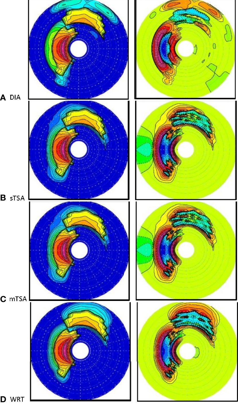
Figure 2 Evolving spectra starting with initial conditions as Figure 1, after time of 5 hours evolution, with no wind: (A) DIA, (B) single-TSA, or sTSA, (C) multiple TSA, or mTSA, (D) WRT, showing 2-D energy in the left column and 2-D Snl in the right. Same color bars and scales as Figure 1. Hs remains constant. Total energy is conserved; Hs is 2.12m.
(c) Evolving Sheared Spectrum, Growing Wind-Sea Opposing Swell Direction
The third test case considers the same initial wave spectrum as in the first case in Figure 1; however there is now a constant west-to-east wind blowing opposite the main westward swell direction, at 20 m/s, with an initial secondary wind-sea to the north, as shown in Figure 1, orthogonal to the assumed wind direction. See Figure 3. The main low-frequency swell direction is to the west. The formulations for wind input, Sin, and wave dissipation, Sds, are given by the ST4 source terms of Ardhuin et al. (2010), as implemented within WW3.
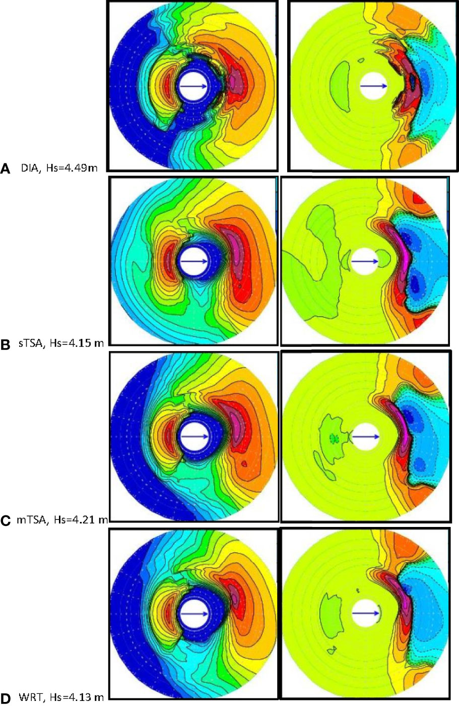
Figure 3 Evolving spectra starting with initial conditions as Figure 1, after time of 10 hours evolution, with 20m/s wind opposing the swell, from west to east and ST4 source terms: (A) DIA, (B) single-TSA, or sTSA, (C) multiple TSA, or mTSA, (D) WRT, showing 2-D energy in the left column and 2-d Snl in the right. Hs (m) as indicated. Same color bars and scales as Figure 1.
Results are shown after the system has evolved for 10 hours. The wind speed of 20 m/s is relatively strong. After 10 hours of time evolution, the new wind-generated waves are the dominant feature in the spectrum of this system. However, in each of the simulations shown in Figure 3, we see that westward propagating swell remains mostly unchanged by the nonlinear transfer Snl, regardless of which formulation is used, WRT, sTSA, mTSA, or DIA. Minor variations are obtained in the swell results, due to DIA formulation and more so in the sTSA results, compared to results from WRT or mTSA.
By comparison, results for the eastward propagating wind-sea driven by 20 m/s wind, imposed on the initial conditions of a northward wind-sea, and a westward propagating swell are a different story. We see that the results for the 2-D action density and the nonlinear transfer Snl, given by mTSA, are largely able to compare to those of WRT relatively well, compared to those of DIA or sTSA. Differences between results of WRT and mTSA are comparatively minor.
By comparison, DIA results have variations in frequency regions around the spectra peak of the northward-propagating wind-sea region. In terms of direction, these effects are most notable in the northeastward direction, approximately diagonal between the northward propagating wind sea, and the new eastward-propagating wind-generated waves. Results from sTSA show notable biases throughout much of the spectrum, although the overall shape of the 2-D action density is rather similar to that of mTSA. For varying 2D distributions, it is not completely clear how to assign a single number to express error. If we take maximum Hs as a kind of qualitative expression of mismatch, then relative to WRT, mTSA has an error of about 1.9% in maximum Hs, compared to 8.7% for DIA.
The overall dominance of the new wind-generated waves propagating to the east is clear after 10 hours. The effects of nonlinear wave-wave interactions between the new wind-generated waves propagating to the east, and the initial conditions involving wind-sea propagating in the northern direction are relatively minor.
(d) Evolving Sheared Spectrum, Growing Wind-Sea Parallel to Initial Wind-Sea
The fourth test case is similar to the third case, except now the 20 m/s wind is blowing south to north, orthogonal to the main east-to-west swell direction, and parallel to the initial secondary wind-sea, also to the north. See Figure 4. The formulations for wind input, Sin, and wave dissipation, Sds, are given by the ST4 source terms of Ardhuin et al. (2010), as implemented within WW3. The simulation is for 5 hr.
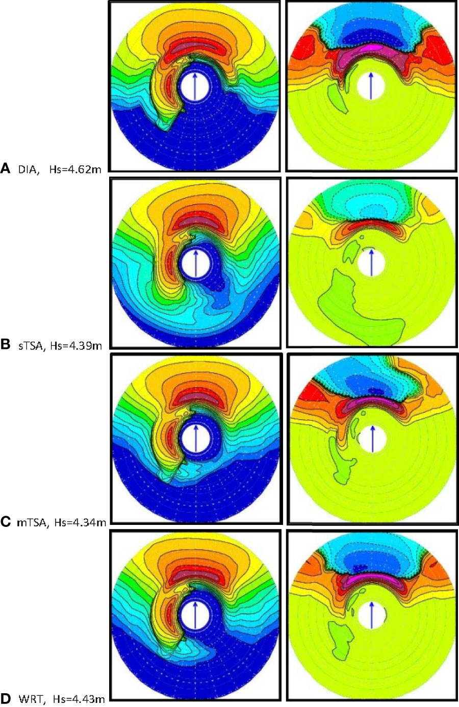
Figure 4 Evolving spectra starting with initial conditions as Figure 1, after time of 5 hours evolution, with 20m/s wind to the north and ST4 source terms: (A) DIA, (B) single-TSA, or sTSA, (C) multiple TSA, or mTSA, (D) WRT, showing 2-D energy in the left column and 2-D Snl in the right. Hs (m) as indicated. Same color bars and scales as Figure 1. Hs is indicated.
As in test case 3, we see that westward-propagating swell remains largely unchanged by the nonlinear transfer Snl, regardless of the formulation; WRT, sTSA, mTSA or DIA. Minor variations are obtained in the swell spectrum due to the DIA formulation, particularly in the southwestern direction, and more so for the results from sTSA, which shows apparent ‘smoothing’ of the westward swell spectrum. Results for the northward propagating wind-sea imposed on the initial conditions and the new generating north-propagating wind-sea waves are dominant features of the simulations.
As in the previous test cases (Figures 1–3), we see again that simulation results given by mTSA are able to match those of WRT rather well, compared to those from DIA or sTSA. By comparison, DIA results have more northerly-propagating wind-sea region and more directional spreading than results suggested by mTSA and WRT; these similar tendencies for more directional spreading and more smoothing are also notable in results from sTSA. The initial wind-sea in the northern direction is effectively ‘assimilated’ into the new wind-generated waves propagating in the northern direction. There is no apparent impact of the west-propagating swell on the newly-generated north-propagating wind-sea.
As in test case 3, the wind speed of 20 m/s is relatively strong, and after 5 hours of time evolution, the new wind-generated waves are the dominant feature in the 2-D spectrum of this system. The effect of the west-propagating swell on the new wind-sea is rather minor and only evident in directional components in the northwest direction, adjacent to the swell propagation direction. However, variations due to differing formulations for Snl are evident. We see that after 5 hours evolution, the results for the simulation given by mTSA are able to match those of WRT relatively well, compared to DIA or sTSA.
By comparison, DIA results have magnitudes that are too large, in both the negative high frequency regions, and also in frequencies of the region around the spectra peak of the north-propagating wind-sea region. In terms of direction, the DIA effects result in more broadly distributed directional spreading of the new wind-sea, rather than to have dominantly north-propagating waves. This tendency of bias and excessive directional spreading is accentuated in the sTSA results. In terms of error, if we take maximum Hs as a qualitative expression for mismatch, then relative to WRT, mTSA has an error of about 2.0% in maximum Hs, compared to 4.3% for DIA.
The overall dominance of the new wind-generated waves propagating northward is clear after the 5-hour time evolution. The effects of nonlinear wave-wave interactions between the new wind-generated waves propagating to the north, and the initial conditions involving swell propagating to the west are relatively minor.
4 Hurricane Teddy (2020)
A detailed discussion of Hurricane Teddy’s development is given by Blake (2021). Teddy began as a strong tropical wave off the west coast of Africa on 10 September, 2020, accompanied by a large area of deep convection, which eventually led to the formation of a tropical depression near 0600 UTC 12 September to the southwest of the Cabo Verde Islands. The “best track” of Teddy’s path is given in Figure 5A. Rapid intensification started late on 15 September and Teddy became a hurricane on 16 September, about 1300 km east-northeast of Barbados as it turned northwestward.
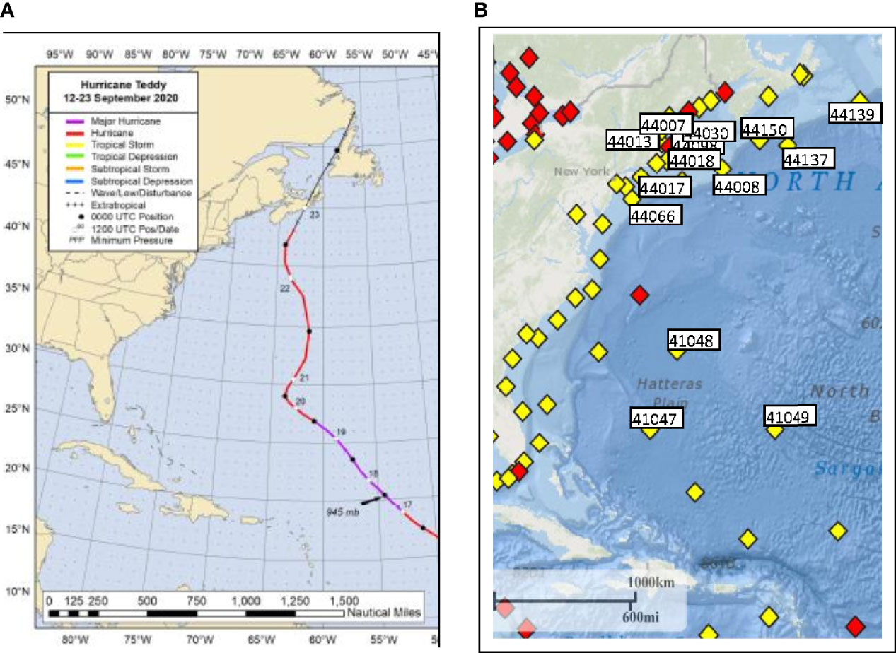
Figure 5 (A) Figure 5 Best track for Hurricane Teddy, 12-23 September 2020. (B) Fourteen NDBC and Canadian buoys used in this study.
By 16 September Teddy’s intensity levelled off at about 85 kt, and with changing shear conditions, it started another intensification by the next day. Teddy strengthened into a major hurricane near 1200 UTC 17 September while centered about 900 km east-northeast of Guadeloupe, reaching a peak of 120 kt near 0000 UTC on 18 September and then beginning to weaken, due to an eyewall replacement, and later due to an increased shear. Teddy dropped below major hurricane status by 0000 UTC 20 September and continued to steadily weaken that day, although its 50-kt and hurricane-force wind fields remained large.
On 20 September, Teddy was centered about 700 km southeast of Bermuda when the synoptic environment changed, causing it to turn northward and then north-northeastward on 21 September, when it passed about 370 km east of Bermuda. The weakening trend stopped late on 21 September due to interactions with a negatively tilted trough, causing an increase in its maximum wind speed and size. Thereafter, Teddy moved rapidly northward and then north-northwestward due to the flow around the trough, and it became a very large cyclone. The extent of tropical-storm-force winds from 0000 UTC 22 September to 1200 UTC that day more than doubled in size in only 12 hours, as confirmed by aircraft and scatterometer data, and a secondary peak intensity of 90 kt between 0600 and 1200 UTC was achieved.
This trough interaction also started Teddy’s extratropical transition process. Teddy’s wind field became more asymmetric, frontal features formed away from the center, and the convection become less centralized. As Teddy moved across cooler water it lost deep convection in the core, and quickly weakened and transitioned to an extratropical low after 0000 UTC 23 September. At this point it was centered about 300 km south of Halifax, Canada. Teddy turned northward and then north-northeastward and made landfall near Ecum Secum, Nova Scotia, Canada, at 1200 UTC that day, with sustained winds of 55 kt. It continued to weaken as it moved across eastern Nova Scotia and the Gulf of St. Lawrence, and was later absorbed by a larger low-pressure system.
Surface wave and meteorological conditions were compared with model estimates at four buoys (41049, 44008, 44137, and 44139) deployed by the National Data Buoy Center (NDBC) and Environment Climate Change Canada (ECCC). These are located in Figure 5B. The peak wind speed at 41049, the most southern of these buoys, was about 22 m/s at 06:00 UTC on Sept 20. Wave conditions increased rapidly as Hurricane Teddy approached, with significant wave heights (Hs) reaching about 9 m at this buoy.
(a) The Wave Model
The computational domain for implementation of WW3 for the simulation of waves generated by Hurricane Teddy consists of the nested grid system shown below in Figure 6. This nested system has a relatively coarse-resolution (0.5°) large-scale grid which extends from 20°N to 65°N, and from 40°W to 75°W for the Northwest Atlantic. Within this domain, a relatively high-resolution subdomain is nested from 42°N to 52°N and from 55°W to 72°W, focused on the waters off northern New England and the Canadian Maritimes Provinces, as shown in Figure 6. These grid resolutions are selected to provide a relatively reliable degree of accuracy in simulating swell and wind-generated waves energy. The directional resolution is 10° and 29 frequency bins are used, spaced logarithmically using fn+1 = 1.10 fn ranging from 0.04118 Hz to 0.5939 Hz. The model global time step is 600 s. As mentioned earlier, the ST4 source terms are used following Ardhuin et al. (2010), for wind input Sin and wave dissipation Sds.

Figure 6 Maps of significant wave height, at the peak of Hurricane Teddy, showing (A) WW3-DIA, (B) WW3-mTSA, (C) WW3-mTSA4, (D) WW3-WRT. Coarse grid (left panel) is at 0.5° resolution and the nested fine-resolution grid (right panel) is 0.1° resolution.
(b) Winds
Wind fields to drive the wave models for Hurricane Teddy are obtained from Environment and Climate Change Canada (ECCC). For the coarse-grid Northwest Atlantic domain, 3-hourly ECCC global wind products are used with 0.24 resolution on a latitude-longitude grid. For the high-resolution Atlantic Canada domain, 1-hourly ECCC regional wind products are used with 10 km resolution based on a polar-stereographic projection. These are routine forecast products that are posted daily by ECCC (https://dd.weather.gc.ca/). The ECCC global wind data are already on a latitude-longitude grid, and so need no further processing. The ECCC regional model has wind components on the polar-stereographic grid of the weather model simulation, and need to be rotated to our latitude-longitude reference frame in order to be ingested into WW3, which then performs interpolations in space and time as needed.
(c) Wave Model Estimates
Figure 6 compares significant wave height distributions from WW3 using the four formulations implemented for the nonlinear wave-wave transfer Snl term. These are the three formulations used in this study; DIA, WRT, and mTSA. A fourth simulation is denoted mTSA4, which uses the tuning for ST4 for the Northwest Atlantic as determined by Perrie et al. (2018); the latter was a study of waves generated by three intense nor’easter storms, and different wave models implemented on coarse- and fine-resolution nested grid systems that are similar to those used in Figure 6. The tuning of ST4 reflects regional characteristics of the Northwest Atlantic and the southern Gulf of Maine, and was shown to give enhanced results.
In these simulations, WW3 is driven by the ECCC wind fields as Teddy propagated from the area around Bermuda, to Nova Scotia as described in the previous section. In terms of the Hs spatial distributions, the results from DIA and WRT appear to exhibit slightly larger Hs values that those of mTSA. However, as expected, this can be compensated for by applying the ST4 tuning suggested by Perrie et al. (2018), which results in higher values in the simulation results for mTSA4.
Overall, the qualitative features of the Hs area distributions and wave directions are similar in these four simulations, with respect to the propagation of the wave fields, the overall directional patterns of the waves, and the peak wave directions. Consistent with fetch-limited growth results reported in previous studies by Perrie et al. (2013), mTSA appears to give results that are biased low, whereas results from DIA are biased high compared to those of WRT, using the standard ST4 source terms. These differences in results from respective different Snl formulations may be somewhat modulated by the inherent nonlinearity, numerical instability etc. present in the WW3 model system.
(d) Comparison of Hs Time Series
To estimate the reliability of the model simulations using the different nonlinear transfer Snl formulations, we conducted comparisons with measured significant wave heights, Hs, with observations at four buoys in the model domain whose locations are shown in Figure 5B. Comparisons were made between time series of buoy measurements of significant wave heights, Hs, and the model simulations for Hurricane Teddy, using the implemented Snl formulations; DIA, mTSA, mTSA4 and WRT. Buoy observations are generally reported at 30-minute intervals.
Figure 7 shows Hs time series and scatter plots at four selected buoys along Teddy’s storm track. These are buoy 41049 near Bermuda, 44008 off Cape Cod, 44137 off Nova Scotia and 44139 near the southern tip of the Grand Banks. These four were selected in order to have additional discussion regarding 1-D and 2-D spectra, in the sections that follow. A summary of statistics for specifically these 4 buoys, plus an additional 10 other buoys along, or near, the storm track of Teddy, indicated in Figures 5A, B is presented in Table 1, in terms of root mean square error (RMSE), bias, correlation coefficient (corr), and scatter index (SI). In this computation of statistics, only data within ± 3 days of the passage of the storm by a given buoy are used; these data are indicated in Figure 7. Note that the full observational time series are indicated by red stars (*), with the points used to calculated statistics (within ± three days of the peak) marked by black circles ʘ overlaying the red stars (*).
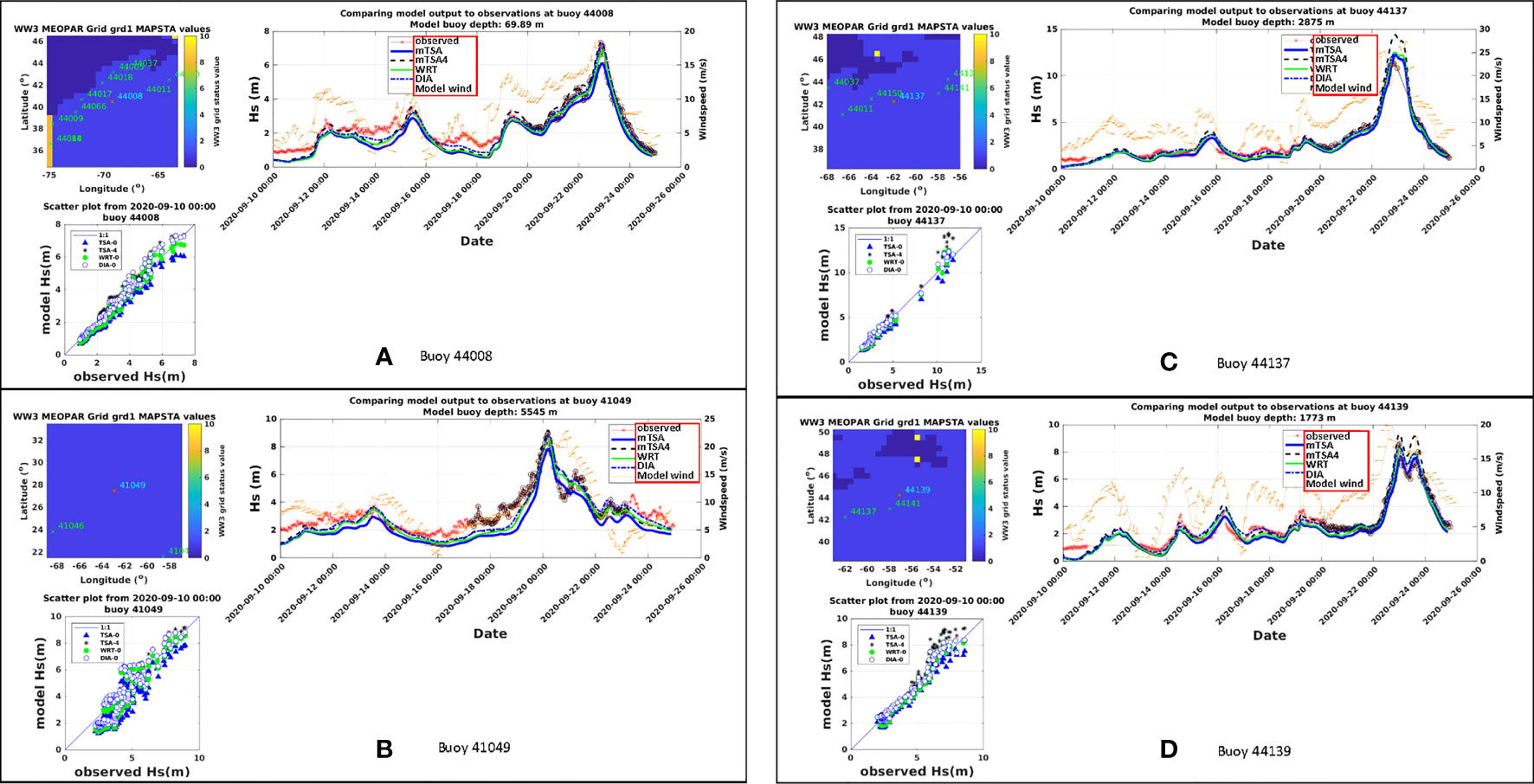
Figure 7 Time series comparisons for significant wave heights Hs for Hurricane Teddy in 2020; shown for buoys: (A) 41049, (B) 44008, (C) 44137, (D) 44139.

Table 1 Statistics for Hs (m) from WW3 wave model compared to measurements at 14 buoys along or near the storm track of Hurricane Teddy, for root mean square error (RMSE), bias, correlation coefficient (corr) and scatter index (SI).
In terms of capturing the storm peak values and model biases, the Hs time series and scatterplots in Figure 7 appear to suggest similar behaviors for all formulations, DIA, mTSA, mTSA4 and WRT. Statistical indices in Table 1 also reflect this finding, with mTSA4 tending to overpredict the peak Hs values and mTSA tending to underpredict these values. This suggests the general approach, that in implementing WW3 for specific regional applications, it important to perform some careful tuning of the basic ST4 source terms of Ardhuin et al. (2010), to reflect the associated regional characteristics. This trend is also reported in the statistical indices in Tables 1 and 2 for the 14 buoys shown in Figure 5B along, or near, Teddy’s storm track. mTSA4 is able to outperform mTSA in terms of improved RMSE, reduced bias, improved correlation coefficient, and scatter index. However, although results from mTSA4 appear to compare somewhat favorably with measurements at buoys 41049 and 44008, the mTSA4 results at buoys 44137 and 44139 appear to have notable overestimates. Thus, the performance is not unequivocal.
Table 2 Statistics for Hs (m) from WW3 wave model compared to measurements at 4 buoys along or near the storm track of Hurricane Teddy, for root mean square error (RMSE), bias, correlation coefficient (corr) and scatter index (SI).
(e) Impacts of Model Tuning
Because ST4 was originally tuned for DIA by Ardhuin et al. (2010) for simulation of waves for global ocean studies it tends to perform well. In fact, statistical indices in Table 1 suggest that DIA can outperform the other simulations; those using mTSA, mTSA4 and WRT. Occasionally, for some of the statistical indices, mTSA4 can outperform the other simulations, for example at buoy 44066 at the edge of the Continental Shelf off the coast of Delaware USA.
As reported by Perrie et al. (2018) the tuning of ST4 consists of adjustments to parameters BETAMAX, the wind-wave growth parameter, and ZALP, the wave age shift of the long waves to account for gustiness, respectively, 1.75 and 0.008, to give optimal simulation skill for waves generated by three nor’easters for the Northwest Atlantic and Gulf of Maine region. It is anticipated that additional tuning could also produce more improvements to the performance of mTSA4. But that is not the objective of this study. In any case, it is interesting to compare the results from mTSA4 with those from mTSA and WRT. Table 2 suggests that for the four selected buoys, results from mTSA4 are generally better than those from WRT or mTSA.
(f) 1-D Wave Spectra
Comparisons between 1-D wave spectra at the peak of the buoy measurements are shown in Figure 8 for Hurricane Teddy. The simulated 1-D spectra are all essentially dominated by single-peaked spectra. Some of the comparisons show large discrepancies between model simulations and observed data. It is evident that as the peak of the storm passes the buoy locations, each will experience changing wind directions, and therefore interactions between swell and wind-waves are present. These interactions are evident in the comparisons that are shown.
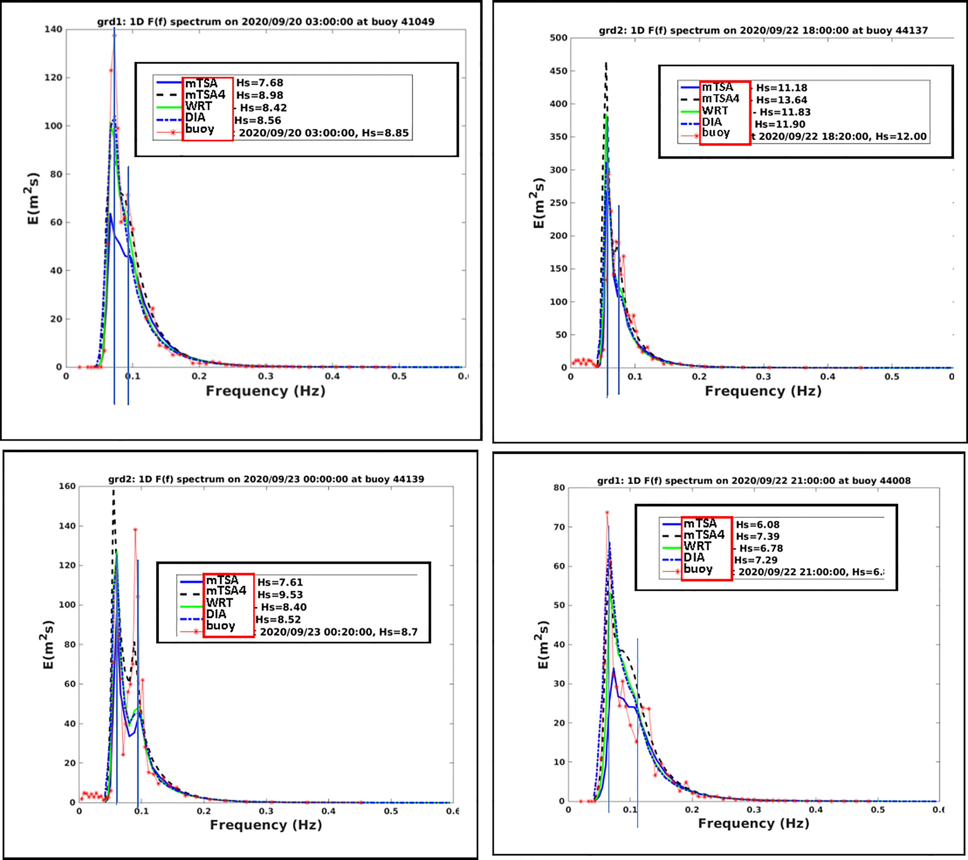
Figure 8 Hurricane Teddy at about the peak of the storm, showing 1D spectrum observed at buoys 41049, 44008, 44137, 44139 compared to simulated results from WW3 with ST4 source terms, DIA, WRT, and mTSA, where mTSA4 assumes the ST4 tuning used in Perrie et al. (2018).
We consider the simulations from the different Snl formulations. Buoy 41049 off Bermuda shows a dominant peak near 0.07 Hz and a secondary peak near 0.09 Hz. Only mTSA4 shows any (minor) indication of the secondary peak. All simulations underestimate the primary peak. mTSA provides a notable underestimate compared to the observations or compared to the other simulations like mTSA, DIA and WRT.
Results for buoy 44008 off Cape Cod are somewhat similar to those of 41049. The observed data indicate some indication of a secondary spectral peak at about 0.11 Hz, and a primary peak at about 0.07 Hz. All model simulations tend to also have indications of the occurrence of the secondary peak, e.g. a ‘wiggle’, but none simulate well the details suggested by the observed data. Also no simulation captures the primary peak, although mTSA4 and DIA appear to come close to so doing, whereas results from WRT and mTSA increasingly underestimate the observed peak data, respectively.
Results for buoy 44137 off Nova Scotia are similar to those of 41049, with a dominant peak around 0.06 Hz and a secondary peak at about 0.08 Hz. Different from the results at 41049, here the results from mTSA4 appear to capture the secondary peak, but notably overestimate results at the primary peak, as do results from WRT. By comparison, results from DIA and mTSA appear to provide a somewhat favorable simulation of the primary spectra peak.
Results for buoy 44139 on the Grand Banks are notable because of the double peak, a low frequency possible swell peak at about 0.06 Hz, and a higher wind-waves peak at about 0.09 Hz. In this case, all the simulations appear to provide some indication of the secondary wind-waves peak, although all present underestimates, with mTSA4 giving the best simulation. For the primary peak, mTSA4 provides an overestimate, whereas the other three manage to give somewhat reasonable simulations.
(g) 2-D Wave Spectra
Comparisons between observed 2D wave spectra and model simulations for Hurricane Teddy at about its peak are shown in Figure 9 for buoys 41049 and 44008. Results for the buoy measurements are calculated following the Longuet-Higgins approximation for the Fourier expansion method as recommended by the NDBC website (www.ndbc.noaa.gov/measdes.shtml). The observed data in Figure 9 at both buoys show the response of the wave spectra to turning winds, as the hurricane passes by and as the primary peak modulates to the new direction of the developing wind-waves.
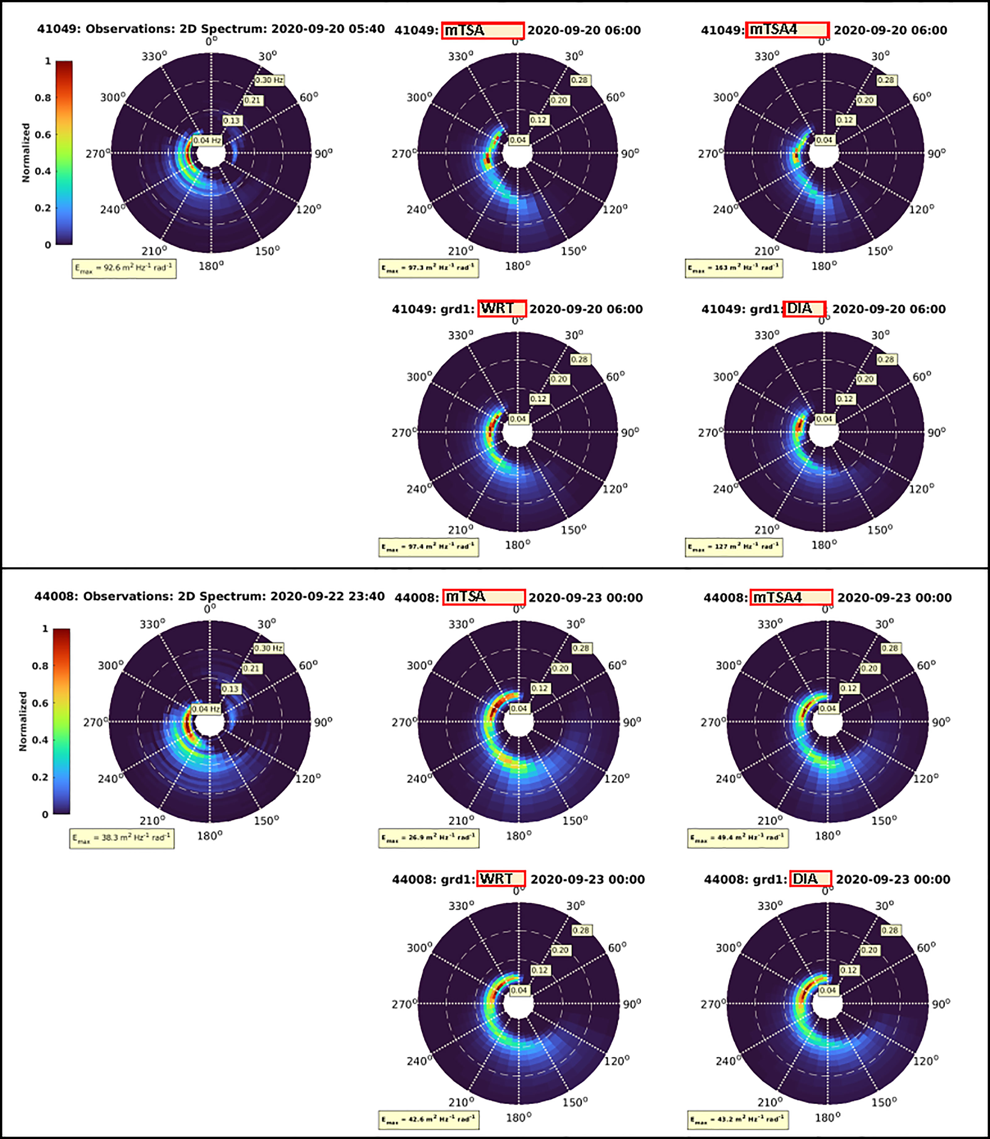
Figure 9 As in Figure 7 for 2D spectrum for Hurricane Teddy at about the peak of the storm, 20 Sept 2020 at 5:40 UTC at buoy 41049, and 22 Sept 2020 at 23:49 UTS at buoy 44008, showing the observed spectrum compared to simulated results from WW3 with ST4 source terms, and DIA, WRT, mTSA4 for nonlinear wave-wave interactions Snl(f, θ). Here, mTSA4 assumes the ST4 tuning from Perrie et al. (2018).
Model simulations suggest qualitatively similar results. Although the observed main directions of the low frequency primary peak and the developing secondary peak are approximately consistent with the simulations, the modelled maximum energy values are generally overestimated compared to the observed values, 92.6 m2Hz-1rad-1 at buoy 41049 and 38.3 m2Hz-1rad-1 at buoy 44008. The model simulations also appear to provide results with wider distributions of new wind-wave energy than is being generated in the new developing wind direction, compared to more restricted directional spreading suggested by the observed spectra. Often it is the other way around, with rather wide directional distributions reported for buoy wave data compared to narrow distributions estimated by wave models. An example of the latter can be found in the comparisons of 2-D modelled and measured spectra by Perrie et al. (2018), which may be attributed to the Longuet-Higgins approximation for the Fourier expansion method.
Overall, the directional distributions resulting for the three Snl formulations do not differ significantly, except in terms of the magnitude of the simulated 2D spectral peaks compared to the observed data. At buoy 41049, magnitudes of peak 2D spectral values are approximately the same as observed, and mTSA4 is too high. See Table 3. At buoy 44008, magnitudes of peak 2D spectral values are approximately the same as observed for results from DIA and WRT, whereas mTSA is too low and mTSA4 is too high. Therefore, as mentioned before, although the ST4 tuning of the two parameters, BETAMAX, the wind-wave growth parameter, and ZALP, the wave age shift of the long waves to account for gustiness, may improve simulations of Hs in Tables 1 and 2, and the 1D spectra in Figure 7, that is not always the case for the 2D spectra.
Table 3 Observed maximum 2-D wave spectra for Hurricane Teddy, compared to simulations.
Another possible constraint on the models is numerics, in terms of the shifting of direction of the spectral peak, and spectral direction distributions. WW3 uses third-order upwind propagation. This is the mechanism that can contribute to the model’s ability to shift the dominant wave directions in response to changing wind directions.
(h) Computational Efficiency
The presentation of results is not complete without mention of computational efficiency. However, the focus of this study has been computational accuracy, rather that computational efficiency. The new mTSA code has not been optimized with MPI (Message Passing Interface) or other methodologies, whereas WRT has had such optimizations. Therefore, in its present formulation, mTSA does not run efficiently. For example, whereas mTSA allows a very large reduction in the number of computations needed to approximate the full integration for the Boltzmann integral for the wave-wave interactions, the separation within the spectrum is presently quite demanding and has not been optimized.
A summary of computational efficiency of mTSA relative to DIA and other formulations for Snl is given in Table 4. In this comparison, FBI is the full Boltzmann integration representation of these quadruplet interactions, which is similar to WRT, and has been used extensively in earlier comparison studies of TSA, such as in Resio and Perrie (2008), with similar run times, ~110 × DIA. By comparison, the present mTSA methodology is about ~100 × DIA, whereas previous older parameterizations of these formulations, FBI-4 and TSA-4, which incorporate alternating frequency and angle computational loops to accelerate the efficiency, and additional parameterizations to attempt improved accuracy, have a computational efficiency in the range of about ~ 26 to 30 × DIA. Future work will focus on optimizing mTSA and the need to enhance computational efficiency.
Table 4 Computational efficiency for the simulation of nonlinear interactions Snl. In this comparison, FBI is the full Boltzman integration representation of nonlinear interactions as used in earlier studies like Resio and Perrie (2008).
5 Discussion and Conclusions
We have considered formulations for the nonlinear wave-wave interactions Snl for application in operational wave forecast models like WAVEWATCHIII™, also denoted WW3. These formulations are DIA formulation from Hasselmann and Hasselmann (1985) and the WAMDI Group (1988), the WRT full integration for the Boltzmann integral based on Webb (1978); Tracy and Resio (1982); Resio and Perrie (1991), and Van Vledder (2006), and the original two-scale approximation, denoted TSA by Resio and Perrie (2008) and Perrie et al. (2013). All of these have been implemented into WW3 in previous studies. Here, in this study, we have proposed a slight generalization of the original TSA, denoted ‘multiple TSA’ or mTSA, to allow better simulation of complicated wave spectra, as may occur in critical situations such as rapidly changing storm situations, shearing spectra, and interactions of swell with wind-waves etc.
To test mTSA, we conduct a variety of test cases, involving hypothetical and real wave spectra. The hypothetical cases are based on a single-point model integration, for complicated wave spectra in interactions between sheared spectra, swell and opposing wind-sea, swell and wind-sea and orthogonal generating wind-waves, etc. which might occur in rapidly changing storm conditions. With respect to the best simulations by WRT, these suggest that the new proposed mTSA is accurate and reliable compared to both DIA, and the previously proposed original version of TSA by Resio and Perrie (2008), which is denoted sTSA in this study. The other source terms used in these tests cases are provided from the ST4 source term formulation of Ardhuin et al. (2010), for example, for wind input Sin and wave dissipation Sds.
We also conducted real test cases, comparing observations from field data with results from simulations with WW3 using these Snl formulations. These test cases are the observations from NDBC and Canadian buoys as collected during Hurricane Teddy in 2020. This storm had its genesis as a strong tropical wave off the west coast of Africa; from there it moved further westward, intensified and then began heading northward from around Bermuda, eventually making landfall in Nova Scotia. Comparisons show that simulations with mTSA, and also mTSA4 with tuned ST4 source terms, are competitive with simulations using DIA or WRT.
Data Availability Statement
Publicly available datasets were analyzed in this study. This data can be found here: Forecast wind products are posted daily to ECCC’s website (https://dd.weather.gc.ca/). NDBC buoy data are available at https://www.ndbc.noaa.gov/.
Author Contributions
WP planned the paper, contributed to the theory design of the TSA model, the test cases and real Hurricane Teddy case, and wrote the paper. BT developed the basic computer codes and ran all the simulations tests. MC performed the pre- and post-processing of data from model simulations, and the visualization of the results. All authors contributed to the article and approved the submitted version.
Conflict of Interest
The authors declare that the research was conducted in the absence of any commercial or financial relationships that could be construed as a potential conflict of interest.
Publisher’s Note
All claims expressed in this article are solely those of the authors and do not necessarily represent those of their affiliated organizations, or those of the publisher, the editors and the reviewers. Any product that may be evaluated in this article, or claim that may be made by its manufacturer, is not guaranteed or endorsed by the publisher.
Acknowledgments
We received funding from the Northeastern Regional Association of Coastal Ocean Observing Systems (NERACOOS), Canada’s Ocean Frontier Institute (OFI), Competitive Science Research Fund (CSRF) and Marine Environmental Observation, Prediction and Response (MEOPAR) to support this development work. Earlier forms of this work were supported by Canada’s Panel on Energy Research and Development (PERD) and US Office of Naval Research. Special thanks to Don Resio for discussion of basic concepts for this work.
References
Ardhuin F., Rogers E., Babanin A. V., Filipot J. F., Magne R., Roland A., et al . (2010). Semi-Empirical Dissipation Source Functions for Ocean Waves. Part I: Definition, Calibration, and Validation. J. Phys. Oceanogr. 40 (9), 1917–1941. doi: 10.1175/2010JPO4324.1
Booij N., Ris R. C., Holthuijsen L. H. (1999). A Third-Generation Wave Model for Coastal Regions, Part 1: Model Description and Validation. J. Geophys. Res. 104 (C4), 7649–7666. doi: 10.1029/98JC02622
Donelan M. A., Hamilton J., Hui W. H. (1985). Directional Spectra of Wind-Generated Waves. Phil. Trans. R. Soc London A 315, 509–562. doi: 10.1098/rsta.1985.0054
Hasselmann K., Barnett T. P., Bouws E., Carlson H., Cartwright D. E., Enke K., et al. (1973). Measurements of Wind-Wave Growth and Swell Decay During the Joint North Sea Wave Project (JONSWAP). Ergänzungsheft zur Deutschen Hydrographischen Zeits. 8 (12), 1–95.
Hasselmann S., Hasselmann K. (1985). Computations and Parametrizations of the Nonlinear Energy Transfer in a Gravity Wave Spectrum, Part I, A New Method for Efficient Computations of the Exact Nonlinear Transfer Integral. J. Phys. Oceanogr. 15, 1369–1377. doi: 10.1175/1520-0485(1985)015<1369:CAPOTN>2.0.CO;2
Holthuijsen L. H. (2007). Waves in Oceanic and Coastal Waters (New York: Cambridge Univ. Press), 387.
Hsiao S.-C., Hongey C., Han-Lun W., Wei-Bo C., Chih-Hsin C., Wen-Dar G., et al. (2020). Numerical Simulation of Large Wave Heights From Super Typhoon Nepartak, (2016) in the Eastern Waters of Taiwan. J. Mar. Sci. Eng. 8 (3), 217. doi: 10.3390/jmse8030217
Komen G. J., Cavaleri L., Donelan M., Hasselmann K., Hasselmann S., Janssen P. A. E. M. (1994). Dynamics and Modelling of Ocean Waves (England, UK: Cambridge University Press), 532 + xxi pages.
Perrie W., Resio D. (2009). A Two-Scale Approximation for Efficient Representation of Nonlinear Energy Transfers in a Wind Wave Spectrum. Part II: Application. To Observed Wave Spectra. J. Phys. Oceanography. 39, 2451–2476. doi: 10.1175/2009JPO3947.1
Perrie W., Toulany B., Resio D. T., Roland A., Auclair J. P. (2013). A Two-Scale Approximation for Wave–Wave Interactions in an Operational Wave Model. Ocean Model 70, 38–51. doi: 10.1016/j.ocemod.2013.06.008
Perrie W., Toulany B., Roland A., Dutour-Sikiric ,. M., Chen C., Beardsley R. C., et al. (2018). Modeling North Atlantic Nor’easters With Modern Wave Forecast Models. J. Geophys. Res. 123 (1), 533-557. doi: 10.1002/2017JC012868
Resio D. T., Long C. E., Vincent C. L. (2004). Equilibrium-Range Constant in Wind-Generated Wave Spectra. J. Geophys. Res. 109, C01018. doi: 10.1029/2003JC001788
Resio D. T., Perrie W. (1991). A Numerical Study of Nonlinear Energy Fluxes Due to Wave-Wave Interactions. Part 1. Methodology and Basic Results. J. Fluid Mech. 223, 609–629. doi: 10.1017/S002211209100157X
Resio D. T., Perrie W. (2008). A Two-Scale Approximation for Efficient Representation of Nonlinear Energy Transfers in a Wind Wave Spectrum, Part 1: Theoretical Development. J. Phys. Oceanogr 38, 2801–2816. doi: 10.1175/2008JPO3713.1
Swail V., Alves JH., Brown J., Greenslade D., Jensen R. (2021). The 2nd International Workshop on Waves, Storm Surges and Coastal Hazards Incorporating the 16th International Workshop on Wave Hindcasting and Forecasting. Ocean Dyn. 71, 957–961. doi: 10.1007/s10236-021-01476-7
Tolman H. (2009) User Manual and System Documentation of WAVEWATCH III™ Version 3.14. Available at: http://polar.ncep.noaa.gov/mmab/papers/tn276/MMAB_276.pdf.
Tolman H. L. (2013). A Generalized Multiple Discrete Interaction Approximation for Resonant Four-Wave Interactions in Wind Wave Models. Ocean Model. 70, 11-24. doi: 10.1016/j.ocemod.2013.02.005
Tolman H. L., Grumbine R. W. (2013). Holistic Genetic Optimization of a Generalized Multiple Discrete Interaction Approximation for Wind Waves. Ocean Model 70, 25–37. doi: 10.1016/j.ocemod.2012.12.008
Tracy B. A., Resio D. T. (1982). Theory and Calculation of the Nonlinear Energy Transfer Between Sea Waves in Deep Water. WES rep. 11, US Army Engineer Waterways Exp. Sta., Vicksburg, MS.
Van Vledder G. P. (2006). The WRT Method for the Computation of Nonlinear Four Wave Interactions in Discrete Spectral Wave Models. Coastal Eng. 53, 223–242. doi: 10.1016/j.coastaleng.2005.10.011
WAMDI Group (1988). The WAM Model – a Third Generation Oceans Wave Prediction Model. J. Phys. Oceanogr. 18, 1775–1810. doi: 10.1175/1520-0485(1988)018<1775:TWMTGO>2.0.CO;2
Webb D. J. (1978). Non-Linear Transfers Between Sea Waves. Deep-Sea Res. 25, 279–298. doi: 10.1016/0146-6291(78)90593-3
WW3DG (WAVEWATCHIII™) Development Group (2016) User Manual and System Documentation of WAVEWATCH III R Version 5.16. Available at: https://polar.ncep.noaa.gov/waves/wavewatch/manual.v5.16.pdf.
Appendix
Given a double-peaked spectrum obtained from observational data such as a buoy, this section provides the procedure for getting the JONSWAP parameters of the two broad-scale terms, the final broad-scale term for the entire spectrum, and the associated local-scale term.
i. The first step is to examine the entire spectrum and find the spectral peak. This is the absolute largest peak. This is the energy maximum. Secondly, this process is repeated and the second spectral peak is determined. This is a local peak, which means it is a local maximum and has at least one frequency bin with lower energy on the left side in a lower frequency bin, and at least one frequency bin with lower energy on the right side, in a higher frequency bin.
ii. Subsequently, just for bookkeeping, the two peaks are labelled so that the lower one on the frequency range is called “fp1” and the other one is “fp2”. Therefore, fp1 is the peak with lower frequency and fp2 is the peak with higher frequency.
iii. The total frequency range is from the lowest frequency in the spectrum, at frequency bin “= one”, or f1, to the highest frequency in the spectrum, which for observed data corresponds to the Nyquist frequency, fNyquist. We divide the frequency range into 2 regions; one for fp1 and one for fp2. The division point is defined by the separation frequency, which is approximated as sitting halfway between the 2 peaks, fp1 and fp2. We do not use optimal fitting to try to somehow refine the splitting of the frequency range between fp1 and fp2, because that reduces the computational efficiency and has not been found to be beneficial. Therefore, the separation frequency is halfway between fp1 and fp2.
iv. The “first region” is from the lowest frequency in the spectrum, f1, to the separation frequency, and the “second region” is from the separation frequency to the highest frequency, fNyquist. For each region, we have one spectrum with one peak. Therefore, we do JONSWAP fitting on each separate region. This is performed by a subroutine (previously developed in the original TSA formulation) that does an optimal five-parameter JONSWAP fitting. Therefore, in the first region for fp1, the five-parameter JONSWAP fitting is done for the frequency sub-range from f1 to the separation frequency. And in the second region for fp2, the five-parameter JONSWAP fitting is also done for the frequency sub-range extending from the separation frequency to the highest frequency, fNyquist. Therefore, we handle the fp1 region and the fp2 region independently.
v. Until now, the JONSWAP fitting is always done in 1-D. To go to 2-D, we apply a directional distribution like ~cosm(θ - θp) to the 1-D parameterizations, at each step, in order to get the two 2-D broad-scale terms for the two regions, for the fp1 region and for the fp2 region, independently.
vi. To get the broad-scale term for the total frequency range, we add together the broad-scale term for the fp1 region, to the broad-scale term for the fp2 region. This completes the fitting for the broad-scale term for the entire frequency range. There is the possibility of a “discontinuity or jump” in the two broad-scale terms at the separation frequency between fp1 and fp2. This is resolved by smoothing, over three frequency bins.
vii. The local-scale spectrum, or residual spectrum is then determined as the difference between the given input spectrum minus the broad-scale term.
Keywords: ocean surface waves, nonlinear wave-wave interactions, two-scale approximation, wind-generated waves, WAVEWATCHIII (WW3) wave model
Citation: Perrie W, Toulany B and Casey M (2022) A Generalized Two–Scale Approximation for Ocean Wave Models. Front. Mar. Sci. 9:867423. doi: 10.3389/fmars.2022.867423
Received: 01 February 2022; Accepted: 06 May 2022;
Published: 30 June 2022.
Edited by:
Adem Akpinar, Uludağ University, TurkeyReviewed by:
Prabhakar V., Vellore Institute of Technology (VIT), IndiaWei-Bo Chen, National Science and Technology Center for Disaster Reduction (NCDR), Taiwan
Prasad Bhaskaran, Indian Institute of Technology Kharagpur, India
Copyright © 2022 Perrie, Toulany and Casey. This is an open-access article distributed under the terms of the Creative Commons Attribution License (CC BY). The use, distribution or reproduction in other forums is permitted, provided the original author(s) and the copyright owner(s) are credited and that the original publication in this journal is cited, in accordance with accepted academic practice. No use, distribution or reproduction is permitted which does not comply with these terms.
*Correspondence: William Perrie, william.perrie@dfo-mpo.gc.ca