Numerical Simulation and Backscattering Characteristics of Freak Waves Based on JONSWAP Spectrum

Introduction

A freak wave, also known as giant wave and rouge wave, is an extremely large wave with hard predictability, short duration, and abnormal wave height in most cases (Fedele, 2016; Wu et al., 2020). Serious marine accidents often occur when a freak wave appears. A freak wave has the above properties and a low probability of occurrence. In the traditional linear or second-order nonlinear wave theory, such extreme waves are almost impossible to form, which makes the design of modern marine explorations, marine engineering structures, and marine vessels often carried out under the conditions of ignoring the freak wave (Residori et al., 2017; Wu et al., 2019a; Latheef et al., 2020; Wang et al., 2020). The freak wave has astonishing destructive power, causing huge losses to the marine economy every year. Therefore, the research on the definition, observation, generation mechanism, evolution, simulation, monitoring, and early warning of freak waves is becoming more and more important.

The formation conditions and locations of freak waves are very wide. Regardless of sea depth or wind scale, there are a large number of unpredictable freak wave observation records in major sea areas such as the Atlantic Ocean, Indian Ocean, North Sea, Sea of Japan, and the surrounding waters of Taiwan. People have not fully understood the generation mechanism of the freak wave. However, most scholars agree that the occurrence probability of a freak wave is higher in deep seas, narrow sea areas, and sea areas with complex seabed topography (Kirezci et al., 2021).

With the gradual improvement of the ocean observation system, the monitoring records of freak waves are also increasing (Amurol and Ewans, 2019; Andrade et al., 2021). However, the suddenness and short-term nature of the freak wave make it difficult to monitor the complete evolution of freak wave. Insufficient experimental data support makes it difficult to effectively do deeper scientific exploration. The simulation research of freak wave is still the focus of the extreme wave research field (Wu et al., 2019; Abroug et al., 2020; Cavaleri et al., 2021). The simulation of the freak wave is mainly numerical simulation, including the random superposition of component waves, the establishment of nonlinear wave numerical models based on evolutionary equations such as KdV equation, Kp equation, and NLS equation, and nonlinear transformation of Stokes waves, etc. We chose the linear wave superposition method to simulate the sea waves.

After sea wave modelling and freak wave are simulated and generated, the effectiveness of freak wave simulation is ensured by comparing its characteristics with the widely recognized definitions of normal wave and freak wave. Further, the construction of the freak wave electromagnetic scattering model is carried out under the previous model, which can analyze the difference in backscattering coefficient between the freak wave and the background wave, and study the relevant characteristics of the electromagnetic scattering of the freak wave.

Numerical Simulation Method of Sea Waves Based on Sea Wave Spectrum

Sea waves are a natural phenomenon with very complicated genesis and evolution (Herterich et al., 2018; Nans and Rónadh, 2020). Sea waves are affected by multiple forces such as gravity, wind, and friction on the seabed, etc. Under the action of external force, the water particle deviates from its original equilibrium state and begins to perform quasi-periodic motion. The action of the fluid makes the regional water particle start to move with it, and its motion state changes periodically with time and space. Through the lowest approximation, sea waves can be regarded as a superposition of countless simple harmonic waves.

Although the physical model-based method in current sea waves simulation research can simulate sea waves from a general hydrodynamic model, its simulations are complex and the amount of simulation is huge, making the model poorly adaptable to practical applications. In fact, because of the strong randomness of the above-mentioned forces, the wave fluctuation cannot be regarded as a simple periodic motion, so it is impossible to describe the motion of the water particle with a specific function.

Numerical simulation of sea waves based on statistical models is a good solution In the mid 20th century, researchers began to treat sea waves motion as a random process. They obtained large amounts of data by arranging experimental equipment in different typical sea areas for long-term observations, and then used probability and statistics theory to analyze the wave motion in different sea areas and different sea conditions. Finally, the random process of sea waves is described in the form of sea wave spectrum (Mendes and Scotti, 2020). Sea wave spectrum is a tool commonly used by relevant personnel for ocean research, as an important statistical feature of the random wave model, it contains important information about the internal and external wave actions of the sea.

From a short-term perspective, wave motion is a stationary random process. We can describe sea waves as the superposition of countless cosine waves, waves of different frequencies have their own amplitudes and contain different energies (Lin et al., 2020; Markov et al., 2021; Shanas et al., 2021). Simulate waves with linear wave superposition method.

$\begin{array}{ll}\eta \left(x,y,t\right)={\displaystyle \sum _{i=1}^M{\displaystyle \sum _{j=1}^N{A}_{ij}sin\left({\omega }_{i}t-k_{i}xcos{\theta }_j-k_{i}ysin{\theta }_j+{\delta }_{ij}\right)}}& (1)\end{array}$

In the formula, each parameter is the state of the component wave at time t. Where A_ij is the amplitude for different component sine waves having wave number k_i, angular frequency ω_i, direction θ_j. According to the linear wave theory, $k_i={\omega }_i^2/g$ A random phase δ_ij. In order to simulate the strong random and irregular waves in the real sea surface, δ_ij is randomly distributed in the interval [0, 2π). The amplitude A_ij is expressed as:

$\begin{array}{ll}{A}_{i,j}=\sqrt{2S\left(\omega ,\theta \right)\Delta \omega \Delta \theta }& (2)\end{array}$

The direction of the wave is influenced by the long-crested wave and the short-crested wave. S(ω, θ) is the directional spectrum of sea waves, also called the directional spectrum function, which is used to describe the composition of the wave direction. It consists of the frequency spectrum S(ω) and the direction function G(ω, θ):

$\begin{array}{ll}S\left(\omega ,\theta \right)=S\left(\omega \right)G\left(\omega ,\theta \right)& (3)\end{array}$

JONSWAP Spectrum

Sea wave spectrum, also called frequency spectrum, is the statistical characteristic of sea waves motion. Common wave spectrums include Neumann spectrum, P-M spectrum, JONSWAP spectrum, Wallops spectrum, Mitsuyasu spectrum, Wen’s spectrum, etc. We compared two common wave spectrums, P-M spectrum and JONSWAP spectrum. It can be seen from Figure 1 that the JONSWAP spectrum is a typical narrow-banded spectrum, which is usually used to generate the 2-D freak waves. The frequency spectrum adopted in the experiment was the JONSWAP spectrum:

$\begin{array}{ll}\begin{array}{c}{S}_j\left(\omega \right)=\frac{\alpha g^2}{{\omega }^5}\text{exp}\left[-\frac{5}{4}{\left(\frac{{\omega }_p}{\omega }\right)}^4\right]{\gamma }^r\\ r=\text{exp}\left[-\frac{{\left(\omega -{\omega }_p\right)}^2}{2{\sigma }^2{\omega }_p^2}\right]\end{array}& (4)\end{array}$

FIGURE 1

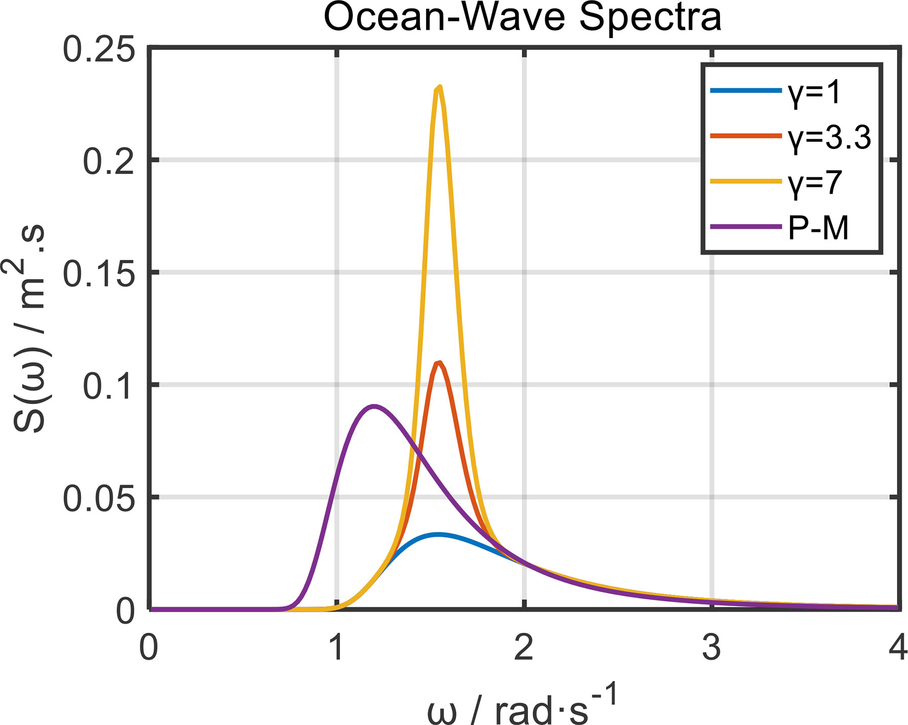
Figure 1 U₁₀ = 7m/s, JONSWAP spectrum for γ=1, γ=3.3, γ=7 and P-M spectrum.

Where α is the energy scale factor, ω_p is the spectral peak circular frequency, σ is the peak shape parameters. $\alpha =0.076{\left(\frac{U_{10}^2}{Fg}\right)}^{0.22}$, ${\omega }_p=22{\left(\frac{g^2}{U_{10}F}\right)}^{1/3}$, σ = 0.07 (ω ≤ ω_p) σ and 0.09 (ω ≥ ω_p). U₁₀ is the wind speed at a height of 10m above the sea surface. F is the distance from a lee shore, called the fetch. As for the extra peak enhancement factor γ: γ = 1 represents the broadband spectrum, γ = 3.3 represents the standard sea-wave spectrum and γ = 7 represents the narrow-banded spectrum.

SWOP Directional Extension Function

This paper selects directional extension function suggested by stereo wave observation project (SWOP). SWOP directional function fully considers the relationship between wavelet direction and spectrum, and the degree of agreement is good. So, its practical application is more extensive:

$\begin{array}{ll}G\left(\omega ,\theta \right)=\frac{1}{\pi }\left\{1+\left[0.5+0.82exp\left(-\frac{{\left(\frac{w}{w_0}\right)}^4}{2}\right)\right]cos2\theta +0.32exp\left(-\frac{{\left(\frac{w}{w_0}\right)}^4}{2}\right)\right\}& (5)\end{array}$

here w₀ = 0.855 × g/U₁₀.

By observing the ideal diagram of the JONSWAP spectrum and SWOP directional extension function under U₁₀ = 7m/s, we selected the appropriate range of angular frequency and direction angle for equal division, and generated a three-dimensional sea surface wave model at a specific time on a given sea area.

Based on Figure 2, we divided 100 component waves according to the frequency equal division method. Each component wave contains 35 equally divided directional angles, which ensures better accuracy and lower simulation volume. All component waves and the direction angles of each component wave participate in the simulation of the sea wave surface. We generated the normal sea surface with U₁₀ = 7m/s:

FIGURE 2

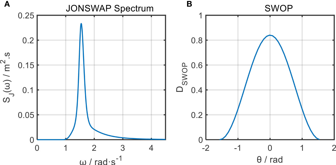
Figure 2 U₁₀ = 7m/s (A) JONSWAP spectrum for γ = 7; (B) SWOP directional extension function.

Numerical Simulation of Extreme 3-D Freak Wave Based on JONSWAP Spectrum and SWOP Directional Extension Function

The JONSWAP spectrum is a classic narrow-banded spectrum, and the component waves have little effect on the wave amplitude when the angular frequency is too high or too low. Theoretically, the amount of calculation for numerical simulation of sea waves is relatively large. Therefore, in this paper we select the appropriate frequency of each component wave which can effectively reduce the amount of calculation. The following figures are in sequence, JONSWAP spectrum, SWOP directional extension function, and Amplitude spectrum. Experiments show that the SWOP directional extension function is affected by the wind speed, and when the wind scale in a high grade, higher energy will be concentrated at the edges:

As shown in Figure 3, the angular frequency of the component wave provides more energy at (1, 1.5), and the energy of the direction angle θ of any component wave reaches the highest at the zero point. In order to reduce the amount of calculation while ensuring the accuracy of the freak wave simulation model, this paper still divides the angular frequency range of the component waves according to the above method, and simulates the freak wave based on the normal sea surface generated before.

FIGURE 3

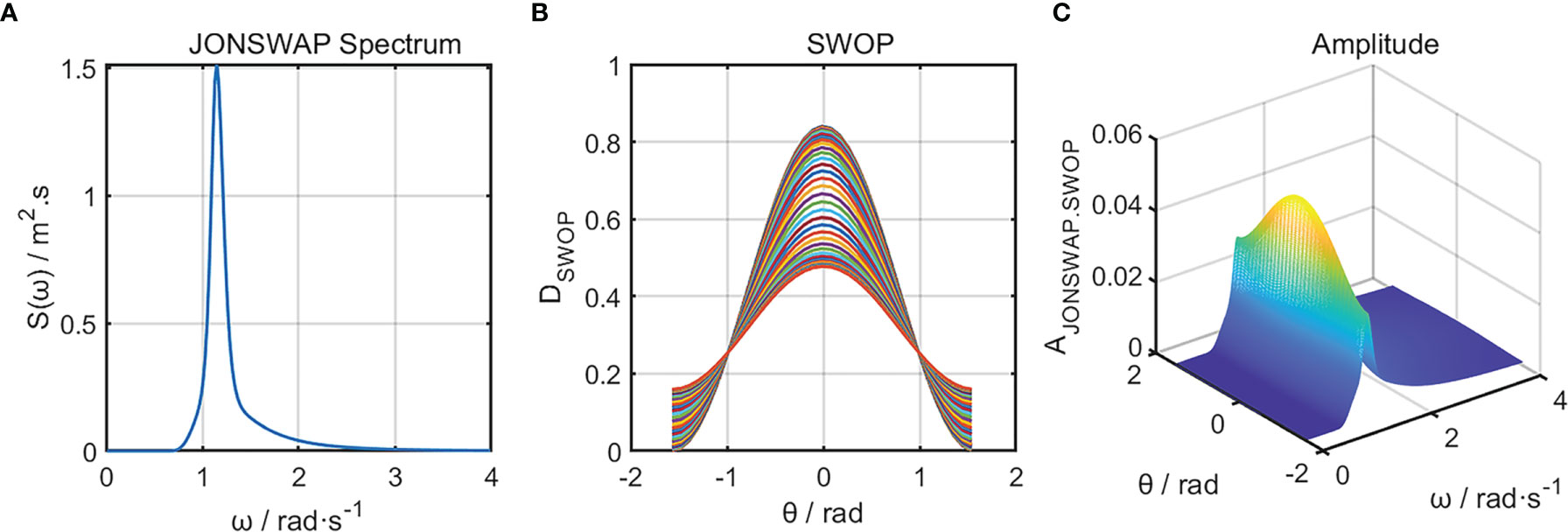
Figure 3 U₁₀ = 17m/s (A) JONSWAP spectrum; (B) SWOP directional extension function; (C) A_{JONSWAP–SWOP} spectrum.

Simulation of the Freak Wave Based on the Principle of Its Generation

Freak wave is a large wave that is unpredictable, short in duration, and giant in wave height. Its specific cause mechanism is far from conclusive. Whether it is an external effect: the continuous transfer of energy in a moving storm to the wave, the change of the wave caused by the complex seabed topography, etc., or the internal evolution: component waves interaction, nonlinear interaction, high-order nonlinear effects, etc. We can see that the essence of generating freak wave is the sudden accumulation of energy, at the moment when the freak wave occurs, the boosted energy of the component wave will be concentrated (Wu and Qiao, 2022; Zeng et al., 2022). Therefore, in the process of numerical simulation of the freak wave, we divide the component wave energies that will produce negative power into different regions, and take them to be positive power proportionally. We make it continuously generate energy to increase the height of the wave crest, and finally complete the experiment of freak wave simulation.

Angular frequency: This paper selected the angular frequency in the range of [0.5, 3], and simulated the average frequency by frequency equal division method numerically. All the component waves participate in the simulation of normal waves. Based on the JONSWAP spectrum, there is more energy when the angular frequency is selected in a specific range. Therefore, this paper selected an appropriate frequency range of angular frequencies (1, 1.5) to make it proportionally concentrate the wave energy in this specific range.

Direction angle: In this paper, we divided the direction angle θ of $\left[-\frac{\pi }{2}, \frac{\pi }{2}\right]$ equally into 35 parts, Δθ = 0.0915. All direction angles of the above-mentioned component waves are involved in normal wave simulation, and some direction angles (–0.75, 0.20) are selected to concentrate energy. Based on the above work, we completed the numerical simulation of the 3-D freak wave surface, by modulating the energy accumulation ratio.

Numerical Simulation of the Extreme Time-Invariant 3-D Freak Wave

In order to have a deeper understanding of freak waves, the researchers conducted observations, collections, and statistical analysis of freak waves that occurred in different areas. In general, there are few measured data used for statistical research of freak waves, but it is still valuable to study the probability distribution of freak waves based on the Gaussian process (Lyu et al., 2021). Whether it is a normal wave or a freak wave, their wave height distribution tends to fit the Rayleigh distribution or the Weibull distribution. Because it has not been decided which distribution is more suitable to fit the wave height distribution, the relevant research is also valuable.

We have simulated simple freak waves (Figure 4). So as to make the freak wave generated in a specific area, and its external characteristics conform to the shape feature of the freak wave, this paper uses Gaussian distribution to realize the adjustment of the proportion of positive energy distribution:

$\begin{array}{ll}f\left(x,y\right)={\left(2\pi {\sigma }_1{\sigma }_2\sqrt{1-{\rho }^2}\right)}^{-1}exp\left[-\frac{1}{2\left(1-{\rho }^2\right)}\left(\frac{{\left(x-{\mu }_1\right)}^2}{{\sigma }_1^2}-\frac{2\rho \left(x-{\mu }_1\right)\left(y-{\mu }_2\right)}{{\sigma }_1{\sigma }_2}+\frac{{\left(y-{\mu }_2\right)}^2}{{\sigma }_2^2}\right)\right]& (6)\end{array}$

FIGURE 4

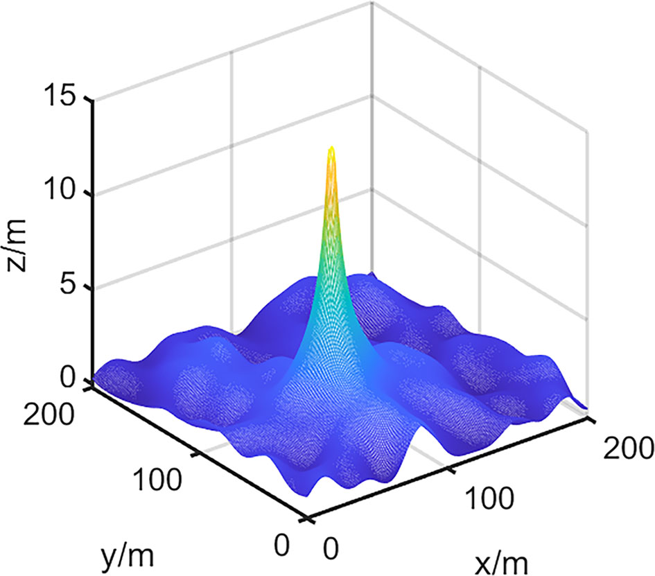
Figure 4 Select a certain area at x=75m, y=75m. Generate freak wave by using energy accumulation method.

Where μ₁, μ₂, σ₁, σ₂, ρ are all constants, μ₁, μ₂ are positional parameters, σ₁, σ₂ are scale parameters and ρ is the tightness parameter. σ₁>0,σ₂>0,|ρ|<1. We say that (X,Y) obey the two-dimensional normal distribution with parameters μ₁, μ₂, σ₁, σ₂, ρ.

To simulate the generation process of the freak wave in chronological sequence, and make freak waves conform to their own characteristics, this paper chooses to use the Rayleigh distribution to dynamically modulate the time evolution of the freak wave, according to the statistical characteristics of the freak wave under the above-mentioned measured data. Probability density of Rayleigh distribution is used as follows:

$\begin{array}{ll}f\left(x\right)=\frac{x}{{\sigma }^2}{e}^{-\frac{x^2}{2{\sigma }^2}},x>0& (7)\end{array}$

Because of its complex formative factors, the conditions and probabilities of the occurrence of the freak wave are different in different sea areas. The freak wave sometimes appears in ordinary sea conditions in some sea areas. However, its occurrence is likely to be accompanied by higher Grade of the Beaufort scale. This paper selects U₁₀ = 17m/s to simulate the evolution of a freak wave surface. The experiment selects γ = 7, F = 40km, U₁₀ = 17m/s.

Figure 5 shows the states of a freak wave at t = 1s, t = 5s, t = 15s, t = 25s, t = 30s, t = 40s, during the whole evolution process. We divided the whole process into three stages: t ∈ (0,5) , the freak wave is in the initial state of evolution, and the freak wave starts to be generated at this stage. When t ∈ [ 5,30 ) , the freak wave is in a fully developed state, and the wave generated at this stage basically satisfies the freak wave definition. t ∈ (30,100) , the freak wave is in the vanishing stage. This series of 3-D simulation figures show the state of the freak wave at different stages. We will verify the accuracy and validity of the above experimental results from several aspects, including wave height distribution, spectrum estimation, and definition of the freak wave, etc.

FIGURE 5

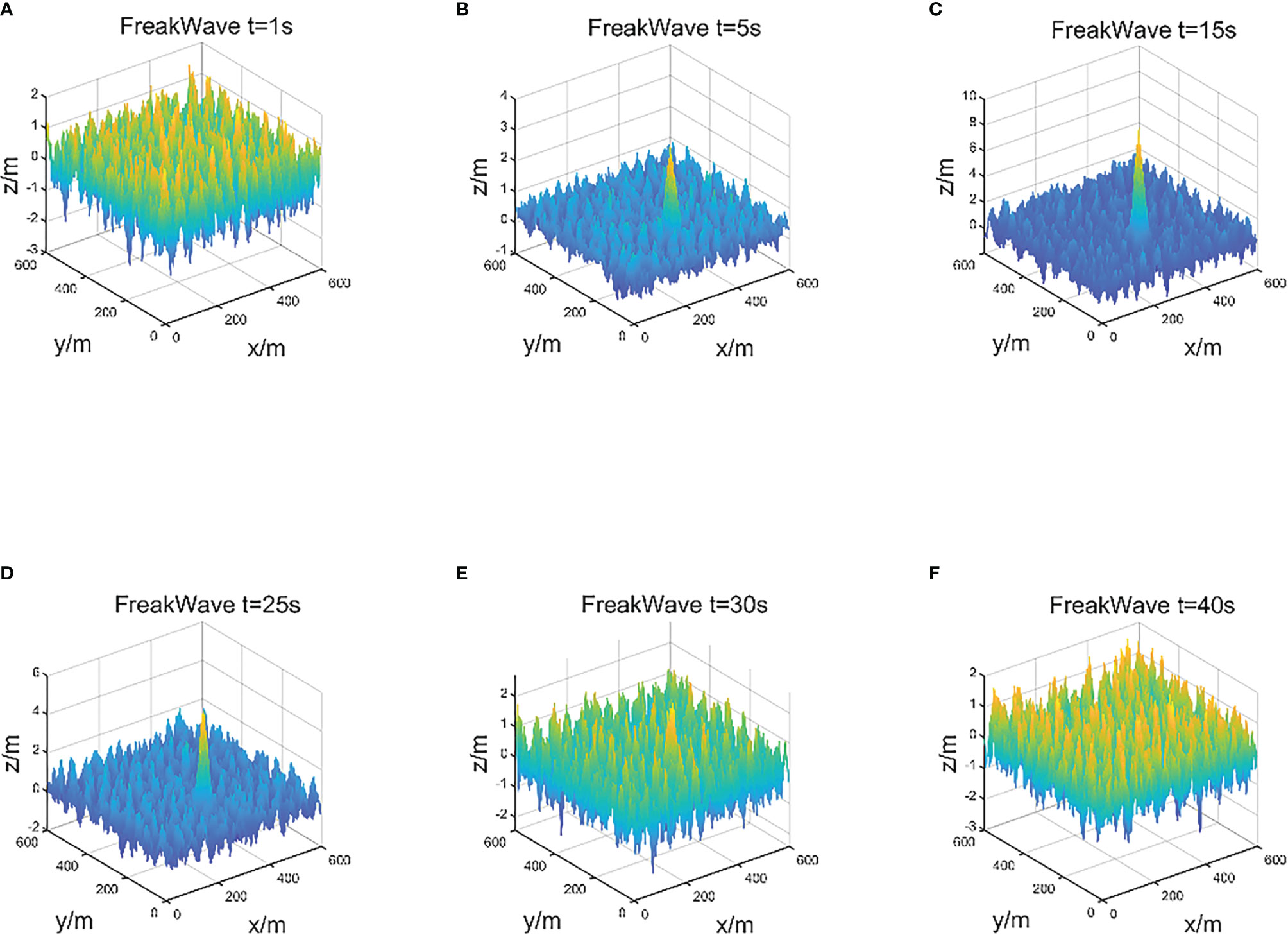
Figure 5 U10 = 17m/s, The evolution of a freak wave on the 600×600 sea area. We recorded six states of the freak wave (A–F) in chronological order.

Experimental Verification of Extreme Time-Invariant 3-D Freak Wave Numerical Simulation Model

After obtaining a complete evolutionary cycle of the freak wave in the experiment, we need to verify the generated freak wave. The simulation verification of the freak wave is mainly to compare with its theoretical model.

We need to verify the normal sea waves generated from the simulation (Figure 6) by comparing and fitting the wave parameters. Wave parameters refer to the external characteristics of sea waves, including wave height, wavelength, period, wave steepness, etc. Research on the statistical distribution characteristics of wave parameters has also achieved many important results. The measured data of the sea help in the construction of the wave model. The verified wave model can in turn provide the basis and experimental data for theoretical research to study the inherent law of the real sea waves.

FIGURE 6

Figure 6 Comparison of the simulated wave spectrum with the target spectrum.

Verification of Wave Height Distribution on Ordinary Sea Surface

Wave height is an important and intuitive wave parameter. It usually refers to the vertical distance between adjacent wave crests and troughs. In actual ocean research and engineering design, the wave height of upward zero-crossing is commonly used.

The statistical distribution characteristics of the wave height can intuitively verify the accuracy of the model. Longuet-Higgins obtained the conclusion that the wave height obeys the Rayleigh distribution under the narrow-banded spectrum assumption (Longuet-Higgins, 1983; Bjørnestad and Kalisch, 2020). This is an idealized wave height distribution model.

For decades, many results have been achieved in the related research on non-Rayleigh wave height distribution, such as probability distribution for wave heights of non-Rayleigh sea waves based on the maximum entropy principle. Nevertheless, these results are often described in complex forms, and the key parameters are difficult to calculate by numerical simulation, which makes it difficult to apply the model to the probability distribution and statistical model of wave height. The Rayleigh distribution describes an idealized state of sea waves (Zhang, 2021). As for the wave numerical simulation based on the JONSWAP spectrum and the SWOP directional extension function, the sea surface numerical simulation model itself is a closed system, which is more ideal than the actual sea surface system (Wu et al., 2019b). So, the Rayleigh distribution can still be used as an important parameter for the verification of wave height distribution (Lim et al., 2021).

In this part, we simulated the ordinary sea surface, and got the state of the sea surface at a certain time during this generation. According to the wave direction, we recorded all the ups and downs of the sea in an area of 600×600, and obtained the wave height using upward zero-crossing method. We sorted the values of wave heights, as shown in the figure:

Based on the data recorded in Figure 7, this paper uses statistical methods to process the wave height data, and compares the probability distribution of the simulated wave height with the theoretically Rayleigh distribution of the wave height. The distribution density function of the wave height is:

$\begin{array}{ll}\begin{array}{cc}f\left(H\right)=\frac{H}{4{\sigma }^2}exp\left(-\frac{H^2}{8{\sigma }^2}\right)& \left(H⩾0\right)\end{array}& (8)\end{array}$

FIGURE 7

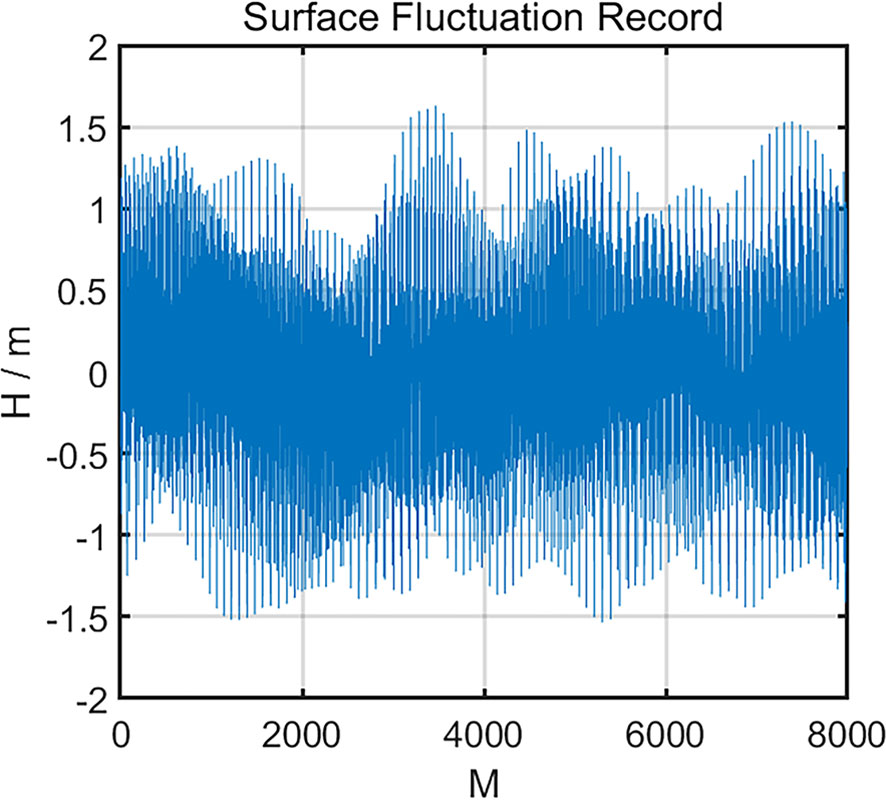
Figure 7 The record of wave surface fluctuation.

H is wave height. σ is the spectral width parameter.

As can be seen from Figure 8 the probability distribution of the wave height data obtained by simulating the ordinary sea surface basically accords with the ideal Rayleigh distribution of wave height, but this also shows that when comparing the wave height distribution, the ideal Rayleigh distribution has the problem that the probability of large waves is too high.

FIGURE 8

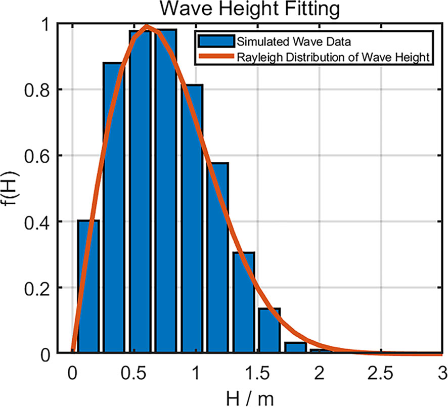
Figure 8 Comparison between the probability distribution of simulated wave height and the theoretical Rayleigh distribution of wave height.

Synthesizing the Figure 8, compared the probability distribution of simulated wave height with the theoretical Rayleigh distribution of wave height, it can be proved that the numerical simulation method of ordinary sea surface proposed above is accurate.

Verification of the Definition of Freak Wave

Since Draper proposed the concept of the freak wave (Draper, 1966), many experts, scholars and marine engineers hope to have a strict definition of it. Barely having the description of the external characteristics of the freak wave can only help people know about the freak wave, but cannot comprehend it. The definition of the freak wave has undergone a period of development. After sorting out a large amount of freak wave data, Klinting and Sand (1987) defined the freak wave as follows:

(1) The wave height H₀ of a single wave is 2 times greater than the significant wave height H_g, H₀/H_s ≥ 2.

(2) The wave height H₀ is greater than or equal to 2 times the wave heights of two adjacent waves H_0–1 and H₀₊₁, H₀/H_0–1 ≥2, H₀/H₀₊₁ ≥2.

(3) The height of the freak wave crest η₀ is greater than or equal to 0.65 times the wave height of this freak wave,η₀/H₀≥ 0.65.

The above is the current internationally recognized definition of the freak wave. This is a relatively strict definition because it not only describes the wave height, but also defines the ratio of the adjacent wave heights and the relationship between the wave height and the wave crest. The freak wave is a large wave different from the background waves, and its wave height usually exceeds 10m, but in mild sea environment the freak wave height may be only about 3m. Considering the uniqueness of the freak wave and its relationship with the background sea state, to avoid confusion with the extreme wave, it is necessary to define the wave shape of the freak wave and the ratio between the freak wave and the adjacent waves. This definition is accepted by most scholars.

The definition of the freak wave is not immutable. Some experts and scholars have added wave steepness to the above definition. In the finite amplitude wave (Stokes) theory, sea waves have a limit wave steepness of 0.142. When the wave steepness is greater than this value, the wave surface will break, that is wave breaking. Mori find that the mean instantaneous wave steepness of breaking waves defined using the zero-down-crossing method was much lower than expected from the Stokes waves (Mori, 2003). While some researchers said that the limit wave steepness of freak wave is higher than 0.142. (Gao et al., 2007) We add the value of wave steepness as the parameter of the freak wave to the parameters that define the freak wave, δ ≤ 0.12, and conduct experiments to analyze its rationality.

This paper selected the above freak wave simulation process Figure 5 to obtain the data, and simulated the five freak wave definitions as the verification parameters numerically. The experimental duration is 40s, U₁₀ = 17m/s, the judgment parameters of the freak wave are named DoF (degree of freak). DoF is the degree of freak. We recorded the characteristic parameter values of the freak wave in the evolution process. The results are as follows:

In the above experiment, A1-A4 are reliable as the judgment parameters, while A5 the wave steepness as a new verification parameter has strong instability, nearly 70% of the experimental results show that A5 is greater than 0.12 and most of them exceed 1.42. A large amount of experimental data show that A5 is often greater than 0.12 when the conditions A1-A4 are met. The causes of the freak wave are complicated. The limit steepness of freak waves in some sea conditions and areas can usually beyond the maximum standard, but no wave breaking occurs. It is obvious that the above limit wave steepness value does not have wide applicability.

The complexity of the ocean itself makes the standard for limit wave steepness of wave breaking not uniform. The limit wave steepness values proposed by many researchers are still different from the observation data of actual freak waves. The wave steepness of the freak wave often exceeds the above standards and without wave breaking. The threshold of limit wave steepness of the freak wave is significantly higher, indicating that conventional breaking conditions cannot be fully applied to the freak wave. Because of this instability, the difference in limit wave steepness between normal wave and freak wave cannot be a standard for defining the freak wave. Compared with normal waves, wave breaking of the freak wave has more powerful destructive force, which is usually dozens of times. Thus, the determination of the wave breaking standard of freak waves needs to be paid attention to.

Verification of the Spectrum Estimation

In this paper, spectrum simulation is used to verify the freak wave numerical simulation model, and the wave data obtained from the wave simulation are used to estimate the spectrum. This paper will observe the fitting degree between the simulated spectrum and the target spectrum, and judge the accuracy of the simulation model based on the fitting results. The following figure is the result of spectrum estimation:

It can be seen from the above comparison result (Figure 9) that the simulated wave spectrum and the target spectrum have a high fitting degree, which indicates that the obtained wave data fits the spectral structure of the target JONSWAP spectrum. The experiment proves that the freak wave numerical simulation model has good spectral fitting degree.

FIGURE 9

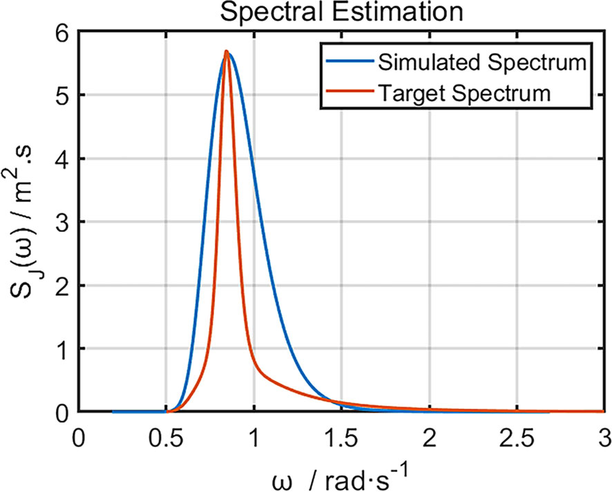
Figure 9 Comparison of the simulated wave spectrum with the target spectrum.

Based on the above experimental data of different verification parameters in Table 1, the numerical simulation model of 3-D freak wave combined with the directional extension function proposed in this paper satisfies the normal JONSWAP spectrum estimation and the verification conditions of the freak wave parameters.

TABLE 1

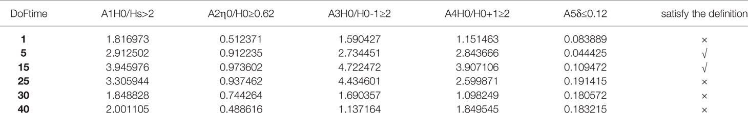
Table 1 Recording and verification of the characteristic parameter values.

Electromagnetic Scattering Simulation of Extreme Time-Invariant 3-D Freak Wave From the Rough Sea Surface

The study of electromagnetic scattering on the 3-D electrical large size sea surface is the focus of actual marine engineering projects (Kotze, 2021). In the study of freak wave, the occurrence and evolution of freak waves can be detected by comparing the SAR imaging of the freak wave with the background wave SAR imaging. The sea surface is a random rough surface. Its state is affected by many factors and cannot be described by an accurate formula. There are many electromagnetic scattering simulation methods, which are mainly divided into two types: approximate method and numerical method.

Numerical method is a method that can get accurate results. Commonly used numerical simulation methods include finite difference method (FDTD), method of moments (MOM), etc. Although there are many improvements based on this way to increase speed and accuracy, even so, the large amount of calculation and limited simulation objects are still a huge limitation, making numerical simulations suitable for low-frequency problems and non-low grazing angles problems. As described, it is difficult to apply to the simulation of electromagnetic scattering from electrical large size sea surface.

The approximate method is to approximate the surface field to a tangent plane, that is, use the tangent plane field of the point to replace the field of the corresponding point. Commonly used approximate methods include Kirchhoff approximation method (KA) and small perturbation method (SPM), small slope approximation method (SSA), integral equation method (IEM). The approximate method is faster and the simulation amount is smaller, but the simulation accuracy is low for large incident angles, and the margin of error is large.

Hybrid method: The rough sea surface is divided into two parts: the large scale that pays more attention to the shape and the small scale that pays more attention to the details. The KA method is suitable for large-scale and the SPM method is suitable for small-scale. The hybrid method combines the above two methods. This common hybrid method called two-scale method (TSM) has the advantages of the two methods, with a wider application range, higher computational efficiency and more accuracy. This is also the focus of current research and the direction of improvement.

In this paper, the classic TSM method in the hybrid method is used to construct an electromagnetic scattering model suitable for the above-mentioned time-invariant 3-D freak wave simulation. We compared the difference of scattering coefficients between freak wave and background wave surface based on the experimental data to analyze the scattering characteristics and identification of the freak wave.

A.K.Fung Wave Spectrum

The waves are not smooth. Large waves are usually covered with gravity waves and capillary waves. In our large number of experiments to study the backscattering characteristics of freak waves, we found that not only gravity waves but also some details of freak waves surface, such as capillary waves (tension waves), breaking waves, etc., will affect electromagnetic scattering. Therefore, in the experimental study of the scattering characteristics of freak waves, we have fully considered the effect of superimposing tension waves on backscattering on the basis of gravity waves.

We use the A.K.Fung wave spectrum to simulate a random rough sea surface to judge the roughness scale. (Fung and Lee, 1982) It is a semi-experienced fully developed wave spectrum based on the gravity spectrum proposed by W.J. Pierson and L.Moskowitz and tension spectrum proposed by W.J. Pierson (Pierson and Moskowitz, 1964). It can be applied to different wave spectra according to the situation. When the wave number in free space K < 0.04rad/cm, the gravity spectrum is used, when K > 0.04rad/cm, the tension spectrum is used, and when K = 0.04rad/cm, the spectral density is equal.

Gravity spectrum W₁(K):

$\begin{array}{ll}{W}_1\left(K\right)=\frac{a_0}{K^3}exp\left(-\frac{b{g}^2}{K^2{u}^4}\right)& (9)\end{array}$

Tension spectrum W₂(K):

$\begin{array}{ll}{W}_2\left(K\right)=0.875{(2\pi )}^{p-1}\left(1+\frac{3K^2}{k_m^2}\right)·g^{\frac{1-p}{2}}{\left[K\left(1+\frac{K^2}{k_m^2}\right)\right]}^{-\frac{p+1}{2}}& (10)\end{array}$

A.K.Fung wave spectrum W(K):

$\begin{array}{ll}W\left(K\right)=\{\begin{array}{ll}{W}_1\left(K\right)\hfill & K<0.04\hfill \\ W_1\left(K\right)\hfill & K>0.04\hfill \end{array}& (11)\end{array}$

Where K is in radians per centimetre. k_m = 3.63rad/cm, g = 981cm/s², a₀ = 1.4 × 10^–3, b = 0.74, p = 5–log(u₁), u₁ is the friction velocity, u is the wind speed at a height of 19.5m above the sea surface $u=\left(u_1/0.4\right)\text{ln}[19.5/(0.684/u_1+4.28\times {10}^{-5}\times u_1^2-0.0443)]\text{cm}/\text{s}$.

The Classic Two-Scale Method

Numerical simulation of electromagnetic scattering from the random rough sea surface. This paper studies on numerical simulation of the backscattering coefficient, and uses the normalized radar cross section (NRCS) to express the electromagnetic wave scattering ability. Under far-field conditions, the scattered power density σ₀ of the element is:

$\begin{array}{ll}{\sigma }_0=\frac{\langle \sigma \rangle }{A_0}=\underset{r\to \infty }{4\pi limr}\frac{\langle {\left|E^s\right|}^2\rangle }{A_0{\left|E^i\right|}^2}& (12)\end{array}$

Where A₀ is the entire area of the random rough sea surface irradiated by electromagnetic waves. σ is Radar cross-sectional area (RCS), r is the distance between the center of the scattering target and the point of the scattering field. Eⁱ is incident field and E^s is scattered field.

Simulate the electromagnetic scattering characteristics of the random rough sea surface numerically, combine KA and SPM, and use the approximate result of the SPM as the scattering coefficient of the small-scale roughness. Perform the ensemble average operation on the slope distribution of the large-scale rough surface to realize the inclination effect of the rough sea surface (Li, 2020). The expression of the backscattering coefficient is:

$\begin{array}{ll}{\sigma }_{pQ}^{TSM}={\sigma }_{pQ}^{KA}\left({\theta }_i,{\theta }_s\right)+\langle {\sigma }_{pQ}^{SPM}\left({\theta }_i^{\text{'}},{\theta }_s^{\text{'}}\right)\rangle & (13)\end{array}$

Where p represents the horizontal or vertical polarization of the scattered field. Q is the horizontal or vertical polarization of the incident field. 〈·〉 means the small-scale wave performs an ensemble average operation based on the surface slope of the large-scale wave.

When the radius of curvature of the large-scale roughness is much larger than the wavelength of the incident electromagnetic wave, KA method approximates the random rough surface to a local tangent plane, and then uses the Fresnel reflection law to solve the total field of the approximate tangent plane, thereby obtaining the far-field approximation Scattered field. Based on the tangent plane approximation theory, the total field strength at any point on the rough sea surface is composed of the incident field and the infinite plane reflection field tangent to this point.

Approximate simulation using Kirchhoff method, only calculating the scattering effect in the direction of the mirror point, ignoring the diffraction effect, through the simulation we get the scattering field expression:

$\begin{array}{ll}{E}^s\left(r\right)=\frac{-jkexp\left(-jk{R}_0\right)}{4\pi R_0}{U}_{PQ}{\displaystyle {\iint }_S{e}^{jk\left(k_s-k_i\right)·r}}dS& (14)\end{array}$

Substituting Equation (14) into Equation (12), the backscattering coefficient of KA is obtained, while θ_i = θ_s,φ_s = π,φ_i = 0:

$\begin{array}{ll}{\sigma }_{pQ}^{KA}\left({\theta }_i,{\theta }_s\right)=\frac{\pi k^2{q}^2}{q_z^4}{\left|U_{PQ}\right|}^{2}P\left(Z_x,Z_y\right)& (15)\end{array}$

Where Z_x = q_x/q_z, Z_y = –q_y/q_z, P(Z_x, Z_y) is the probability density slope distribution function. U_pQ is the polarization coefficient, it can be calculated by the Fresnel reflection coefficient. When calculating backscattering, it is simulated numerically based on the Fresnel reflection coefficient R_hh, R_vv, the formula is:

$\begin{array}{ll}\{\begin{array}{l}{R}_{hh}=\frac{cos{\theta }_i-\sqrt{\epsilon -si{n}^2{\theta }_i}}{cos{\theta }_i+\sqrt{\epsilon -si{n}^2{\theta }_i}}\hfill \\ R_{vv}=\frac{{\epsilon }_{r}cos{\theta }_i-\sqrt{\epsilon -si{n}^2{\theta }_i}}{{\epsilon }_{r}cos{\theta }_i+\sqrt{\epsilon -si{n}^2{\theta }_i}}\hfill \end{array}& (16)\end{array}$

ε is the relative permittivity of sea water.Use the SPM method to simulate the electromagnetic scattering coefficient of the small-scale rough surface numerically, and add the simulation result to the electromagnetic scattering simulation result of the large-scale rough surface (ensemble average operation) to simulate the total scattering coefficient (Wu et al., 2017). Under the conditions of the SPM method, the incoherent scattering cross section per unit area of the random rough sea surface is:

$\begin{array}{ll}{\sigma }_r=\frac{4}{\pi }{k}^{4}co{s}^2{\theta }_{i}si{n}^2{\theta }_s\mid a{\mid }^{2}W\left(p,q\right)& (17)\end{array}$

Where k is the incident wave number, θ_i is the incident angle, θ_s is the scattering angle, a is the polarization coefficient under hh or vv. In the case of backscattering θ_i =θ_s, φ_s = π, φ_s, is the scattering azimuth, so a_vh = a_hv = 0, ε is the relative permittivity of sea water, then the expression is:

$\begin{array}{ll}\{\begin{array}{l}{a}_{hh}=\frac{\left(\epsilon -1\right)}{{\left[cos{\theta }_i+{\left(\epsilon -si{n}^2{\theta }_i\right)}^{\frac{1}{2}}\right]}^2}\hfill \\ a_{vv}=\frac{\left(\epsilon -1\right)\left[\left(\epsilon -1\right)si{n}^2{\theta }_i\right)+\epsilon ]}{{\left[cos{\theta }_i+{\left(\epsilon -si{n}^2{\theta }_i\right)}^{\frac{1}{2}}\right]}^2}\hfill \end{array}& (18)\end{array}$

W(p, q) represents the power spectrum density:

$\begin{array}{ll}W\left(p,q\right)=\sqrt{2}\pi {\sigma }_{0}2l^2{\left(1+K^2{l}^2\right)}^{-\frac{3}{2}}& (19)\end{array}$

Where σ₀ represents the root-mean-square surface height of rough sea, l is the correlation length surface height of rough sea, K is the spatial wave number, so the formula is:

$\begin{array}{ll}{\sigma }_r=\frac{\sqrt[4]{2}}{\pi }{k}^2{\sigma }_{0}2co{s}^4{\theta }_i\mid a{\mid }^2{\left(1+k^2{l}^2\right)}^{-\frac{3}{2}} & (20)\end{array}$

Backscattering coefficient of electromagnetic wave on the random rough sea surface.

$\begin{array}{ll}\sigma =10log{\sigma }_r& (21)\end{array}$

Electromagnetic Scattering Characteristics Analysis of the Freak Wave Surface

After the verified freak wave numerical simulation model was used to generate the freak wave, the TSM method was used to simulate the electromagnetic scattering coefficient of the 3-D freak wave sea surface. Set condition parameters, U₁₀ = 17m/s, the length of the wind zone 1000m, ε = 81, Radar frequency 2.8GH_Z, polarization HH. Usually we use the high resolution and low grazing angle radar to observe the freak wave. In this paper, the radar incident wave we selected is close to the grazing incidence state, Radar incident angle 89.3512. In order to distinguish the speckle noise on the real radar image (about 10–20dB in magnitude), the enhanced NRCS values of background wave and the freak wave are shown in the figures:

Analyze the electromagnetic scattering coefficient of the 3-D freak wave and compare the NRCS of the background sea surface. The above experiment Figure 10 shows that the NRCS value is the lowest at the place where the freak wave is generated.

FIGURE 10

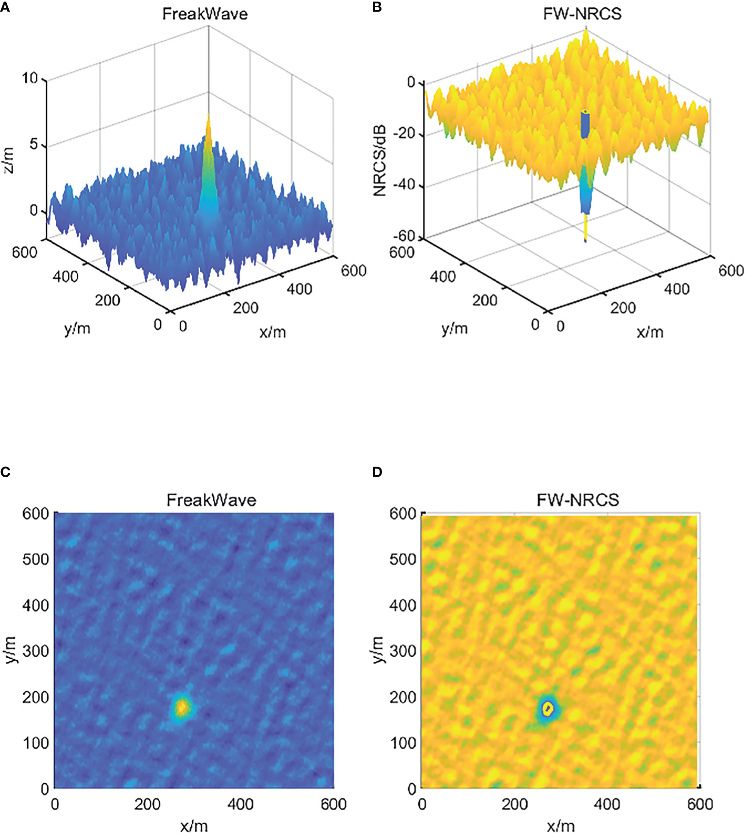
Figure 10 (A) 3-D freak wave with wavelength 91m and wave height 10.96m and the random rough sea surface; (B) the freak wave and the background wave NRCS; (C) top view of the random rough sea; (D) top view of NRCS on the sea.

We conducted experiments and recorded the NRCS values for the two types of sea waves (background wave, freak wave). We compared the lowest NRCS values of the two waves, and the average NRCS values around them. We did complete experiments and recorded the average values. The experimental data are as follows:

Analysing the NRCS difference between the freak wave and the background wave in the above experimental results, it can be seen from the Table 2 that the difference is obvious. Therefore, the NRCS difference can be used as a judgment to identify the freak wave. According to the above experimental data, the identification threshold of the freak wave should be 30dB. The ocean is a complex system, and the corresponding identification thresholds under different ocean conditions require a lot of experiments to summarize.

TABLE 2

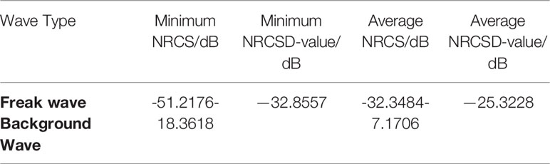
Table 2 Comparison of NRCS values of two different types of wave.

It should be noted that, at the critical positions of different roughness scales, the transition of the electromagnetic scattering coefficient is unstable and not smooth. This is because the TSM method mechanically divides the sea surface which in the real world as a whole system into large-scale gravity waves and small-scale tension waves for processing. It destroys the integrity and smoothness of the system. The correct representation of the two-scale and the smoothness of the transition need to be further improved.

Conclusions

In this paper, the extreme time-invariant 3-D freak wave surface is generated by modulation on the random rough sea surface which is simulated based on the sea wave directional spectrum combined with the JONSWAP spectrum and the SWOP directional extension function. The essence of generating freak wave is the sudden accumulation of energy, when the freak wave occurs, the boosted energy of the component wave will be concentrated. So, in the process of numerical simulation, we turn the component wave energy that will produce negative values, named Negative Energy, into Positive Energy proportionally to increase the height of the wave crest. And through observation, a large number of measurement data show that the evolution of the freak wave shows a certain trend with time. We regulate the energy in chronological order to simulate the occurrence of the freak wave.

After obtaining the 3-D freak wave numerical simulation model, we verified the freak wave by wave height distribution fitting and spectrum estimation. Moreover, by using the widely recognized freak wave definition as verification parameters, and adding wave steepness as a new parameter, the generated freak wave was verified. After verifying the parameters, we found that the wave steepness of the freak wave as a new verification parameter, its value has strong instability. Compared with normal sea waves, the threshold of limit wave steepness of the freak wave is significantly higher, so the wave breaking characteristics of it can be a standard for defining the freak wave. The freak wave has strong destructive power after breaking, we need to pay more attention to the determination of the wave breaking standard of the freak wave.

We conducted a study on the electromagnetic scattering of the freak wave on the random rough sea surface, and used the TSM model to study the electromagnetic scattering characteristics of the freak wave and the background wave. The experimental data shows that the NRCS of the freak wave is much smaller than the NRCS of the background sea waves. The above-mentioned verification parameters for defining the freak wave are too dependent on the measured data of sea waves. In actual engineering, sea surface electromagnetic scattering engineering is more efficient. We take the NRCS difference as the judgment condition to identify the freak wave. According to the above experimental data, the identification threshold of the freak wave should be 30dB. However, as mentioned above, the generation and evolution of the freak wave are complicated, and the specific range of NRCS difference that defines the freak wave needs to be determined by further research.

Data Availability Statement

The raw data supporting the conclusions of this article will be made available by the authors, without undue reservation.

Author Contributions

All authors contributed to the research in this paper. Data curation, LH; Formal analysis, GW; Investigation, GW; Methodology, LZ; Software, LH; Writing – original draft, LH; Writing – review and editing, GW. All authors contributed to the article and approved the submitted version.

Funding

This work is supported by the Natural Science Foundation of Shandong Province, China, grant number ZR2021MD063.

Conflict of Interest

The authors declare that the research was conducted in the absence of any commercial or financial relationships that could be construed as a potential conflict of interest.

Publisher’s Note

All claims expressed in this article are solely those of the authors and do not necessarily represent those of their affiliated organizations, or those of the publisher, the editors and the reviewers. Any product that may be evaluated in this article, or claim that may be made by its manufacturer, is not guaranteed or endorsed by the publisher.

References

Abroug I., Abcha N., Dutykh D., Jarno A., Marin F. (2020). Experimental and Numerical Study of the Propagation of Focused Wave Groups in the Nearshore Zone. Phys. Lett. A. 384, 126144. doi: 10.1016/j.physleta.2019.126144

CrossRef Full Text | Google Scholar

Amurol S., Ewans K. (2019). The Effect of Swell on Wave Spectra of Extreme Sea States Offshore Sarawak, Malaysia. Ocean. Eng. 189, 106288. doi: 10.1016/j.oceaneng.2019.106288

CrossRef Full Text | Google Scholar

Andrade D., Stuhlmeier R., Stiassnie M. (2021). Freak Waves Caused by Reflection. Coast. Eng. 170, 104004. doi: 10.1016/j.coastaleng.2021.104004

CrossRef Full Text | Google Scholar

Bjørnestad M., Kalisch H. (2020). Extreme Wave Runup on a Steep Coastal Profile. AIP. Adv. 10 (10), 105205. doi: 10.1063/5.0020128

CrossRef Full Text | Google Scholar

Cavaleri L., Barbariol F., Bastianini M., Benetazzo A., Bertotti L., Pomaro A., et al. (2021). An Exceptionally High Wave at the CNR-ISMAR Oceanographic Tower in the Northern Adriatic Sea. Sci. Data 8, 37. doi: 10.1038/s41597-021-00825-x

PubMed Abstract | CrossRef Full Text | Google Scholar

Draper L. (1966). ‘Freak’ Ocean Waves. Weather 21 (1), 2–4. doi: 10.1002/j.1477-8696.1966.tb05176.x

CrossRef Full Text | Google Scholar

Fedele F. (2016). Are Rogue Waves Really Unexpected? J. Phys. Oceanogr. 46 (5), 1495–1508. doi: 10.1175/JPO-D-15-0137.1

CrossRef Full Text | Google Scholar

Fung A., Lee K. (1982). A Semi-Empirical Sea-Spectrum Model for Scattering Coefficient Estimation. IEEE J. Ocean. Eng. 7 (4), 166–176. doi: 10.1109/JOE.1982.1145535

CrossRef Full Text | Google Scholar

Gao P., Wang L., Zhao X. (2007). Study on Characteristics of Freak Wave. China Harb. Eng. 2007 (6), 28–31. doi: 10.3969/j.issn.1003-3688.2007.06.009

CrossRef Full Text | Google Scholar

Herterich J., Cox R., Dias F. (2018). How Does Wave Impact Generate Large Boulders? Modelling Hydraulic Fracture of Cliffs and Shore Platforms. Mar. Geol. 399, 34–46. doi: 10.1016/j.margeo.2018.01.003

CrossRef Full Text | Google Scholar

Kirezci C., Babanin A. V., Chalikov D. V. (2021). Modelling Rogue Waves in 1D Wave Trains With the JONSWAP Spectrum, by Means of the High Order Spectral Method and a Fully Nonlinear Numerical Model. Ocean. Eng. 231, 108715. doi: 10.1016/j.oceaneng.2021.108715

CrossRef Full Text | Google Scholar

Klinting P., Sand SE (1987). Analysis of prototype freak waves. Coastal Hydrodynamics. ASCE, 618–32.

Google Scholar

Kotze P. (2021). Monsters of the Seas. New Scient. 249 (3327), 41–45. doi: 10.1016/S0262-4079(21)00523-6

CrossRef Full Text | Google Scholar

Latheef M., Abdullah M. N., Jupri M. F. M. (2020). Observed Spectrum in the South China Sea During Storms. Ocean. Dynam. 70 (3), 353–364. doi: 10.1007/s10236-019-01332-9

CrossRef Full Text | Google Scholar

Li D. (2020). Research on Electromagnetic Scattering Characteristics of Nonlinear Sea Surface. Ph.D. Dissertation (Chengdu City, Sichuan Province, China: University of Electronic Science and Technology of China).

Google Scholar

Lim C., Lee J. L., Lee S. (2021). Analyzing Wave Height and Direction Using the Rayleigh Distribution Function. J. Coast. Res. 114 (SI), 534–538. doi: 10.2112/JCR-SI114-108.1

CrossRef Full Text | Google Scholar

Lin S., Sheng J., Xing J. (2020). Performance Evaluation of Parameterizations for Wind Input and Wave Dissipation in the Spectral Wave Model for the Northwest Atlantic Ocean. Atmosphere-Ocean 58, 258–286. doi: 10.1080/07055900.2020.1790336

CrossRef Full Text | Google Scholar

Longuet-Higgins M. S. (1983). On the Joint Distribution of Wave Periods and Amplitudes in a Random Wave Field. Proc. R. Soc. Lond. Ser. A. Math. Phys. Sci. 389 (1797), 241–258. doi: 10.1098/rspa.1983.0107

CrossRef Full Text | Google Scholar

Lyu Z., Mori N., Kashima H. (2021). Freak Wave in High-Order Weakly Nonlinear Wave Evolution With Bottom Topography Change. Coast. Eng. 167, 103918. doi: 10.2208/kaigan.76.2_I_1

CrossRef Full Text | Google Scholar

Markov N., Nikolov G., Kishev R. (2021). Numerical and Experimental Generation of Freak Waves. Eng. Sci. LVIII 2 68–78. doi: 10.7546/EngSci.LVIII.21.02.06

CrossRef Full Text | Google Scholar

Mendes S., Scotti A. (2020). Rogue Wave Statistics in (2+1) Gaussian Seas I: Narrow-Banded Distribution. Appl. Ocean. Res. 99, 102043. doi: 10.1016/j.apor.2019.102043

CrossRef Full Text | Google Scholar

Mori N. (2003). Effects of Wave Breaking on Wave Statistics for Deep-Water Random Wave Train. Ocean. Eng. 30, 205–220. doi: 10.1016/S0029-8018(02)00017-3

CrossRef Full Text | Google Scholar

Nans B., Rónadh C. (2020). Maximal Heights of Nearshore Storm Waves and Resultant Onshore Flow Velocities. Front. Mar. Sci. 7. doi: 10.3389/fmars.2020.00309

CrossRef Full Text | Google Scholar

Pierson W. J., Moskowitz L. (1964). A Proposed Spectral Form for Fully Developed Wind Seas Based on the Similarity Theory of SA Kitaigorodskii. J. Geophys. Res. 69 (24), 5181–5190. doi: 10.1029/JZ069i024p05181

CrossRef Full Text | Google Scholar

Residori S., Onorato M., Bortolozzo U., Arecchi F. (2017). Rogue Waves: A Unique Approach to Multidisciplinary Physics. Contemp. Phys. 58(1), 53–69. doi: 10.1080/00107514.2016.1243351

CrossRef Full Text | Google Scholar

Shanas P. R., Kumar V. S., George J., Joseph D., Singh J.. (2021). Observations of Surface Wave Fields in the Arabian Sea Under Tropical Cyclone Tauktae. Ocean. Eng. 242, 110097. doi: 10.1016/j.oceaneng.2021.110097

CrossRef Full Text | Google Scholar

Wang Y., Xu F., Zhang Z. (2020). Numerical Simulation of Inline Forces on a Bottom-Mounted Circular Cylinder Under the Action of a Specific Freak Wave. Front. Mar. Sci. 7. doi: 10.3389/fmars.2020.585240

CrossRef Full Text | Google Scholar

Wu L., Breivik Ø., Rutgersson A. (2019a). Ocean-Wave-Atmosphere Interaction Processes in a Fully Coupled Modeling System. J. Adv. Model. Earth Syst. 11 (11), 3852–3874. doi: 10.1029/2019MS001761

CrossRef Full Text | Google Scholar

Wu G., Liang Y., Xu S. (2019). Numerical Computational Modeling of Random Rough Sea Surface Based on JONSWAP Spectrum and Donelan Directional Function. Concurr. Comp-Pract. E. 33, 1–15. doi: 10.1002/cpe.5514

CrossRef Full Text | Google Scholar

Wu L., Qiao F. (2022). Wind Profile in the Wave Boundary Layer and Its Application in a Coupled Atmosphere-Wave Model. J. Geophys. Res.: Ocean. 127 (2), e2021JC018123. doi: 10.1029/2021JC018123

CrossRef Full Text | Google Scholar

Wu L., Shao M., Sahlée E. (2020). Impact of Air–Wave–Sea Coupling on the Simulation of Offshore Wind and Wave Energy Potentials. Atmosphere 11 (4), 327. doi: 10.3390/atmos11040327

CrossRef Full Text | Google Scholar

Wu G., Song J., Fan W. (2017). Electromagnetic Scattering Characteristics Analysis of Freak Waves and Characteristics Identification. Acta Phys. Sinica. 66 (13), 134302(1–10). doi: 10.7498/aps.66.134302

CrossRef Full Text | Google Scholar

Wu L., Staneva J., Breivik Ø., Rutgersson A., Nurser A. J., Clementi E., Madec G., et al. (2019b). Wave Effects on Coastal Upwelling and Water Level. Ocean. Modell. 140, 101405. doi: 10.1016/j.ocemod.2019.101405

CrossRef Full Text | Google Scholar

Zeng F., Zhang N., Huang G., Gu Q., Pan W., et al. (2022). A Novel Method in Generating Freak Wave and Modulating Wave Profile. Mar. Struct. 82, 103148. doi: 10.1016/j.marstruc.2021.103148

CrossRef Full Text | Google Scholar

Zhang H. (2021). Numerical Analysis on Three-Dimensional Green Water Events Induced by Freak Waves. Ship. Offsh. Struct. 16, 33–43. doi: 10.1080/17445302.2021.1894030

CrossRef Full Text | Google Scholar