An analytic model of typhoon wind field and simulation of storm tides

1 Introduction

The frequency of typhoon activity in the Northwestern Pacific Ocean has increased in response to rising sea surface temperatures, attributed to global climate warming (Chan and Liu, 2004; Wu et al., 2005; Chan, 2007). Ocean heat, mainly represented by sea surface temperatures, plays a crucial role in the formation and development of typhoons. In addition, rising sea levels due to global warming have exacerbated vulnerability to storm tide disasters, further exacerbating the problem (Karim and Mimura, 2008; Woodruff et al., 2013).

Numerical modelling and data analysis are essential tools for predicting typhoons/hurricanes and associated storm tides. Pressure and wind derived from reanalysis data are commonly used for storm tide simulations (Brenner et al., 2007; Zhang and Sheng, 2015; Dullaart et al., 2020). However, analyses have shown that wind speeds near the maximum wind radius (MW) of the cyclone are often underestimated when compared to actual measurements (Carvalho, 2019; Çalışır et al., 2021).

Parametric wind models are crucial for efficiently simulating storm tides, providing pressure and wind speed profiles (Lin and Chavas, 2012; Torres et al., 2019; Vijayan et al., 2021). These models typically consist of two components: pressure and wind speed profiles. Wind speed or pressure formulas can be derived from each other based on the gradient wind equation, allowing for the construction of different parametric models (Jelesnianski, 1965; Holland, 1980; Wang et al., 1991).

While numerous studies have focused on simulating storm surges (Sun et al., 2015; Ramos Valle et al., 2018; Sun and Zhong, 2018), the issue of storm current velocities (SCV) has received limited attention. Challenges arise from the difficulty in observing SCV during typhoons/hurricanes and obtaining accurate wind profiles from previous parametric models.

This study proposes a new analytic model for the typhoon wind field, which is validated against measured wind profile data. A mathematical model of storm tides, driven by the wind stress derived from the new model, is established and compared with observed data on storm surges and SCVs during Typhoon Rammasun. The performance of the new model in simulating SCVs is also compared to previous models. Temporal and spatial variations of storm tides during Typhoon Rammasun are analyzed.

2 An analytic model of typhoon wind field

2.1 Wind models

Table 1 provides a comprehensive list of various parametric wind models used in storm tide simulations. Parametric wind models are developed based on the differential equation of the gradient wind, employing two different approaches: (1) deriving wind profiles by differentiation based on assumed pressure profiles, as exemplified by the widely used Holland model, and (2) deriving pressure profiles by integration after assuming wind profiles, as exemplified by the Jelesnianski model (Table 1).

TABLE 1

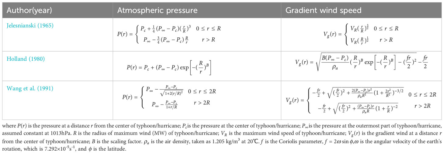
Table 1 Different parametric wind models.

The pressure formula in the Jelesnianski (1965) wind model was obtained by integrating the differential equation of the gradient wind under the assumption of a relative speed profile. However, this model has certain limitations, including the neglect of Coriolis and resistance forces and the unknown maximum speed V_R. Wang et al. (1991) suggested the “Fujita-Takahashi” model, combining Fujita’s pressure formula for r< 2R and Takahashi’s formula for r > 2R, as a suitable option for simulating storm surges in China. However, this model exhibited a discontinuity in the wind profile at 2R and was inconsistent with physical phenomena. Holland (1980) derived a wind speed formula using the Mayer pressure profile, which is more physically reasonable compared to the above models. However, the drag term in the wind differential equation was neglected, resulting in an overestimation of wind speeds.

2.2 A new analytic model of typhoon

Accurate estimation of wind speed is crucial for the simulation of SCVs during typhoon/hurricane events. However, the lack of suitable wind models has hindered our ability to predict SCVs accurately.

The gradient wind results from the interaction of multiple forces, including the horizontal pressure gradient force, the Coriolis force, the centrifugal force, and the drag force at the air-sea interface. To address the limitation of three wind models above, a sea surface drag term was taken into account in the following differential equation

$\begin{array}{ll}\frac{V_g^2}{r}+V_{g}f-\frac{1}{{\rho }_a}\frac{\partial P}{\partial r}+gJ=0& (1)\end{array}$

where potential energy slope $J$ is determined by the sea surface drag relationship

$\begin{array}{ll}J=\frac{\lambda }{4R_w}\frac{V_w^2}{2g}& (2)\end{array}$

where $V_w$ is the flow velocity, $R_w$ is the hydraulic radius, $\lambda$ is the water drag coefficient.

According to the boundary layer theory, an extremely thin fluid layer with a large velocity gradient should exist in the moving air at the sea-air interface, in which viscosity plays a very important role. And in this boundary layer, there is an inner laminar layer closer to the sea surface that maintains laminar flow. The narrow layer of laminar flow exists closely near the air-sea interface, where the viscous shear stress prevails so that the drag coefficient of laminar flow is adopted as follows

$\begin{array}{ll}\lambda =\frac{6}{\mathrm{Re}}=\frac{6\nu }{R_w{V}_w}& (3)\end{array}$

The combination of eq.(2) and eq.(3) yields the following

$\begin{array}{ll}gJ=\frac{3}{4}\frac{\nu }{R_w^2}{V}_w& (4)\end{array}$

Similar to eq.(4), we get the air drag

$\begin{array}{ll}gJ=\frac{3}{4}\frac{\nu }{{\delta }_a^2}{V}_g& (5)\end{array}$

where $\nu$ represents the kinematic viscosity of air taking as 15.8×10^-6m²/s; $V_g$ represents the gradient wind speed; hydraulic radius is assumed to be ${\delta }_a$, the thickness of the laminar air flow at sea-air interface. ${\delta }_a$ is a coefficient related to wind speed and is a constantly changing quantity in a real typhoon wind field. According to theoretical calculations, the magnitude of ${\delta }_a$ is 10^-1m. In practice, ${\delta }_a$ is determined as a uniform value and can be adjusted according to the typhoon.

By substituting eq.(5) into eq.(1), the gradient wind equation considering the sea surface drag can be expressed as follow

$\begin{array}{ll}\frac{V_g^2}{r}+V_{g}f-\frac{1}{{\rho }_a}\frac{\partial P}{\partial r}+\frac{3}{4}\frac{\nu }{{\delta }_a^2}{V}_g=0& (6)\end{array}$

Eq.(6) presents a univariate quadratic equation about $V_g$ that is the most important parameter in wind model. $V_g$ can be obtained by solving eq.(6) when pressure profile $P(r)$ is known. According to approach (1), we employed Mayer pressure profile to eq.(6) for the sake of convenience

$\begin{array}{ll}P(r)=P_c+(P_{\infty }-P_c)\exp (-R/r)& (7)\end{array}$

Therefore, the gradient wind formula considering sea-surface drag is obtained

$\begin{array}{ll}{V}_g(r)=\sqrt{\frac{(P_{\infty }-P_c)R}{{\rho }_{a}r}\exp \left[-(\frac{R}{r})\right]+\frac{{(f+3\nu /4{\delta }_a^2)}^2{r}^2}{4}}-\frac{(f+3\nu /4{\delta }_a^2)r}{2}& (8)\end{array}$

$V_g(r)$ represents the magnitude of the gradient wind at any distance r from typhoon center. For any pressure profile, we can obtain the corresponding gradient wind profile.

Letting r = R in eq.(8) gives the maximum gradient wind V_max

$\begin{array}{ll}{V}_{\max }=\sqrt{\frac{(P_{\infty }-P_c)}{{\rho }_{a}e}+\frac{{(f+3\nu /4{\delta }_a^2)}^2{R}^2}{4}}-\frac{(f+3\nu /4{\delta }_a^2)R}{2}& (9)\end{array}$

The typhoon speed, displaying an asymmetry distribution, consists of gradient and moving winds, in which magnitude of gradient wind meets eq.(8).

There are different types of models for representing the moving wind that is generated by the movement of the typhoon center (Jelesnianski, 1965; Ueno, 1966). The Ueno formula, widely used, was selected for the moving wind

$\begin{array}{ll}{V}_m=V_c\exp (-\frac{\pi }{4}\frac{\left|r-R\right|}{R})& (10)\end{array}$

where $V_c$ is the moving speed of a typhoon center.

The gradient wind vectorially superimposed with the moving wind so that we obtained the speed vector

$\begin{array}{ll}\{\begin{array}{c}{V}_{rx}=\frac{V_g}{r}[-(x-x_c)\sin \theta -(y-y_c)\cos \theta ]+V_{cx}\exp (-\frac{\pi }{4}\frac{\left|r-R\right|}{R})\\ V_{ry}=\frac{V_g}{r}[(x-x_c)\cos \theta -(y-y_c)\sin \theta ]+V_{cy}\exp (-\frac{\pi }{4}\frac{\left|r-R\right|}{R})\end{array}& (11)\end{array}$

where $V_{rx}$ and $V_{ry}$ are the components of wind speed in the $x$ and $y$ direction at a distance $r$ from the center of typhoon, $r=\sqrt{{(x-x_c)}^2+{(y-y_c)}^2}$; $\theta$ is the incidence angle of the gradient wind; $V_{cx}$ and $V_{cy}$ are the components of the moving wind speed in the $x$ and $y$ directions.

The radius of MW is an important parameter in wind models. We construct the formula for R considering dimensional harmony

$\begin{array}{ll}R=R_{\min }{e}^{k(P_c/P_{\min }-1)}& (12)\end{array}$

where $P_{\min }$ is the minimum typhoon central pressure measured in the nearshore waters of China, taken as 895 hPa; $R_{\min }$ is the mean radius of MW corresponding to $P_{\min }$, taken as 27.9 km; and k is an adjustable constant, that may be taken as 10.5 according to limited data.

2.3 Observed data and validation of wind models

The wind profiles of two hurricanes, Tracy (Director of Meteorology, 1977) and Joan (Director of Meteorology, 1979), observed by the Bureau of Meteorology Australia, were utilized to validate the present wind model and other existing models. Hurricane Tracy made landfall in Darwin with a minimum pressure of 950 hPa and MW of 38 m/s on 24-25 December 1974. Hurricane Joan, with a minimum pressure of 930 hPa and MW of 40 m/s, crossed Port Hedland on 8 December 1975. The wind profile of Typhoon Betty was also obtained from the China Meteorological Administration. Additionally, wind speeds at Chunxiao platform during Typhoon Rammasun were observed by the Second Institute of Oceanography, State Oceanic Administration, from 2-6 July 2002. In the calculations, the scale factor B of Holland model are 1.05, 1.5, 1.16 and 1.05 in case Joan, Tracy, Betty and Rammasun respectively, while the ${\delta }_a$ are 0.15m, 0.1m, 0.25m and 0.15m respectively.

Comparisons between the calculated wind profiles using the present wind model and the measured profiles during hurricanes Tracy, Joan, and Typhoon Betty demonstrated excellent agreement, as depicted in Figure 1. Furthermore, the wind speed variations over time, computed using the present wind model and the central pressure of Typhoon Rammasun during 2-6 July, exhibited a high level of concordance with the observed data, as illustrated in Figure 2. For comparison, the results obtained from the Holland and Fujita-Takahashi wind models were also included in Figures 1, 2.

FIGURE 1

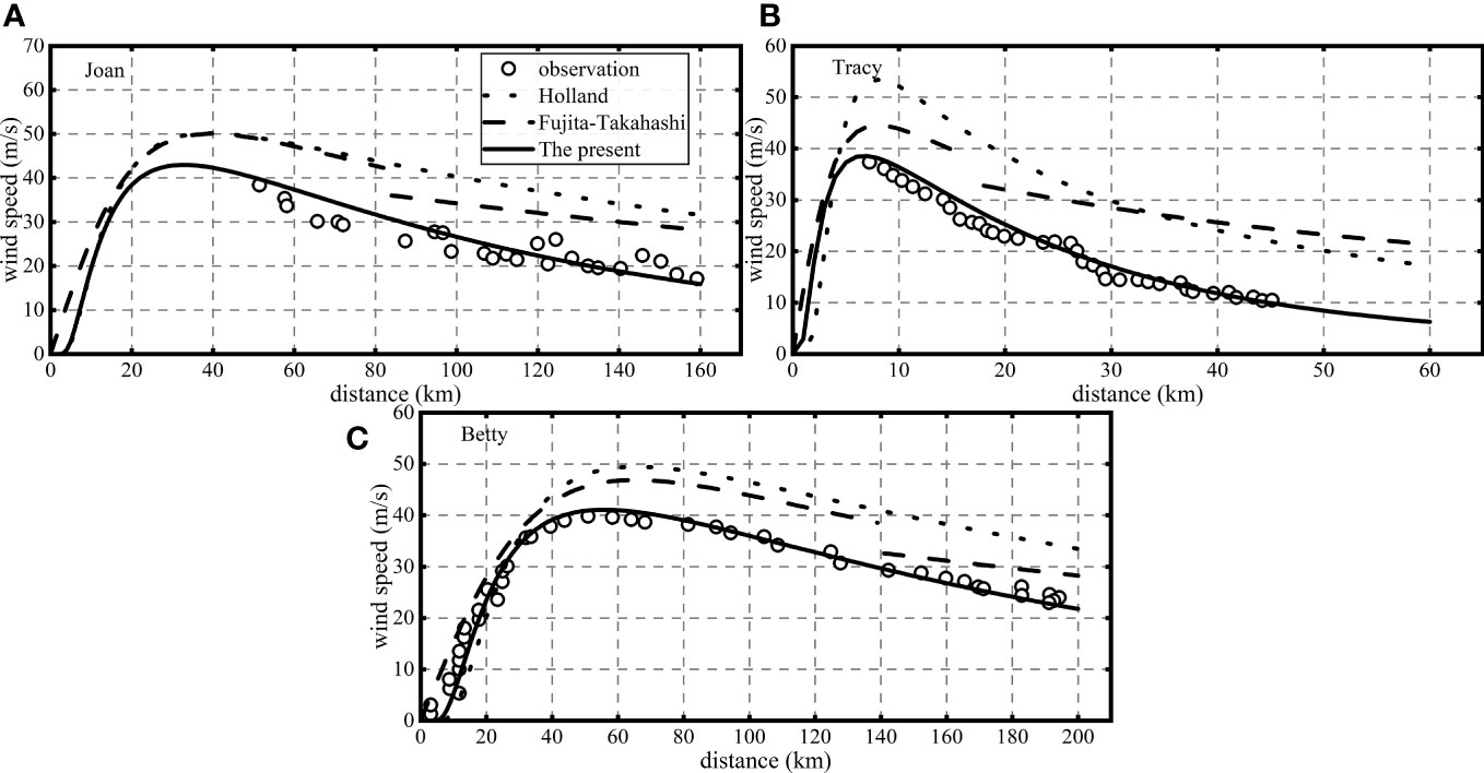
Figure 1 Comparison of wind speed calculated from the present and Holland, Fujita-Takahashi model with the measured. (A) Hurricane Joan, (B) Hurricane Tracy, (C) Typhoon Betty.

FIGURE 2

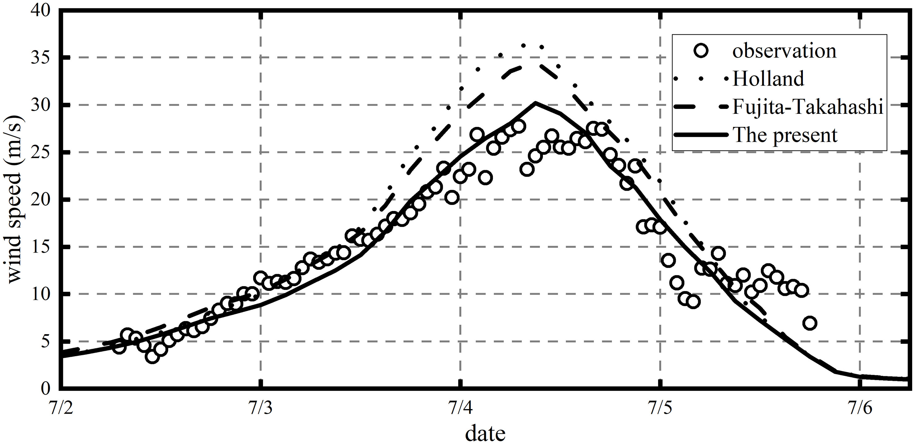
Figure 2 Comparison of wind speed calculated from the present and Holland, Fujita-Takahashi model with the measured during Typhoon Rammasun.

To assess the reliability and accuracy of the models, commonly used metrics such as root mean square error (RMSE) and skill score (SS) were employed (Sun et al., 2015)

$\begin{array}{ll}RMSE={[\frac{1}{N}{\displaystyle \sum _{i=1}^N{(s_i-o_i)}^2}]}^{1/2}& (13)\end{array}$

$\begin{array}{ll}SS=1-\frac{{\displaystyle {\sum }_{i=1}^N{(s_i-o_i)}^2}}{{\displaystyle {\sum }_{i=1}^N{(\left|s_i-{\overline{o}}_i\right|+\left|o_i-{\overline{o}}_i\right|)}^2}}& (14)\end{array}$

where $o_i$ and $s_i$ are the observed and simulated value at point i. N presents the number of points. $\overline{o_i}$ and $\overline{s_i}$ are the average observed and simulated value. The smaller RMSE indicates the smaller deviation between the simulated and the observed values, while SS closer to 1 indicates a better agreement between the simulated and observed values.

Figure 1A illustrates the comparison of wind calculations during Hurricane Joan obtained from different models with the corresponding observations. The RMSEs for the three models are 14.62 m/s, 10.86 m/s, and 2.93 m/s respectively. Remarkably, the errors associated with the present model are significantly lower than those of the other models. The SS of the present model reaches 0.94, indicating the highest level of agreement with the measured values. In contrast, the SS values for the Holland and Fujita-Takahashi models are 0.48 and 0.61 respectively. These results highlight the superior predictive accuracy of the present model compared to the other models.

Similarly, Figures 1B, C depict the verification of wind profiles during Hurricane Tracy and Typhoon Betty. In these cases, the present model exhibits an impressive SS value of 0.99, indicating significantly higher accuracy compared to the other two models. These findings underscore the superiority of the present model in accurately predicting wind profiles during hurricanes/typhoons, surpassing the performance of the Holland and Fujita-Takahashi models.

Furthermore, Figure 2 presents the temporal variation of winds at a fixed station during Typhoon Rammasun. The results demonstrate that the present model achieves high accuracy, with an SS value of 0.97 and an RMSE of 2.6 m/s. In contrast, the Holland and Fujita-Takahashi models exhibit RMSE values of 5.36 m/s and 4.25 m/s respectively. Notably, the present model excels in accurately calculating the MW with a relative error of only 2.88%. In comparison, the relative errors for the Holland and Fujita-Takahashi models are 20.89% and 14.94%.

The above analyses clearly demonstrate the superior performance of the present model in accurately predicting wind profiles, thus providing a solid basis for predicting SCV during hurricanes/typhoons Table 2.

TABLE 2

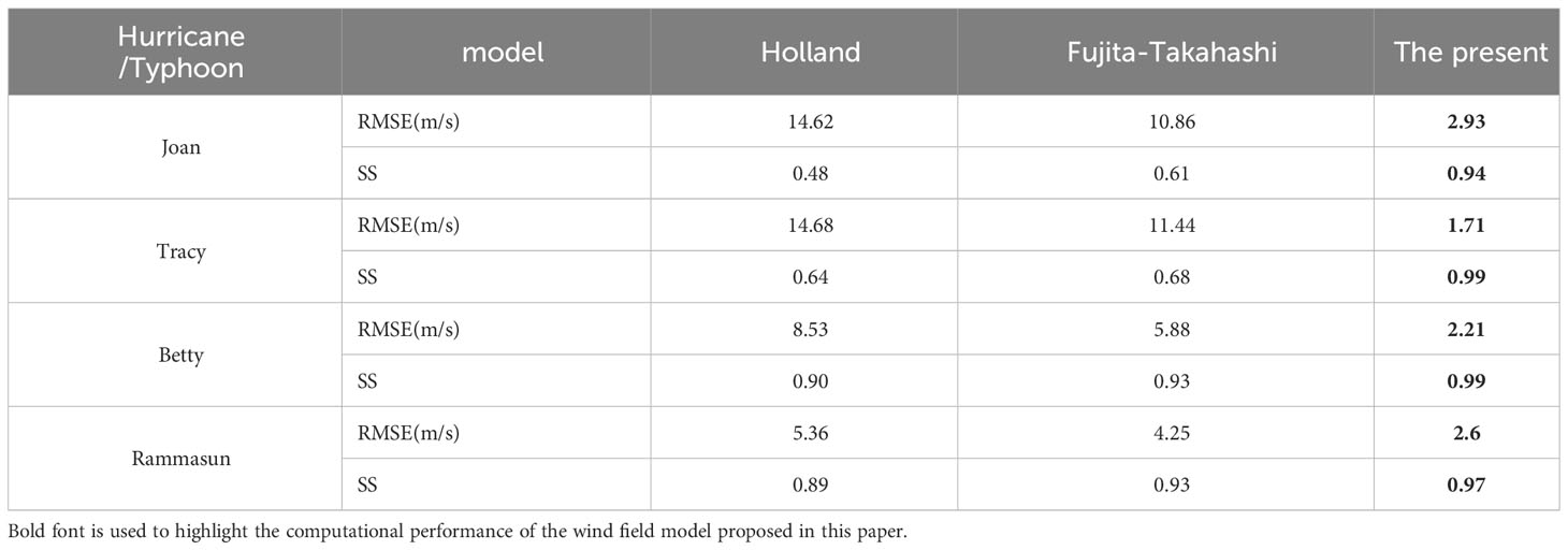
Table 2 Verification of wind speed simulated from various models.

3 Storm tide simulation and verification

3.1 Governing equations and wind input

A mathematical model of typhoon storm tides was established on basis of Delft3D (Roelvink and Van Banning, 1995), where the governing differential equations include

Continuity equation

$\begin{array}{ll}\frac{\partial \zeta }{\partial t}+\frac{1}{\sqrt{G_{\eta \eta }}\sqrt{G_{\xi \xi }}}\frac{\partial \left((d+\zeta )U\sqrt{G_{\eta \eta }}\right)}{\partial \xi }+\frac{1}{\sqrt{G_{\eta \eta }}\sqrt{G_{\xi \xi }}}\frac{\partial ((d+\zeta )V\sqrt{G_{\xi \xi }})}{\partial \eta }=0& (15)\end{array}$

Momentum equations

$\begin{array}{ll}\begin{array}{l}\frac{\partial u}{\partial t}+\frac{u}{\sqrt{G_{\xi \xi }}}\frac{\partial u}{\partial \xi }+\frac{v}{\sqrt{G_{\eta \eta }}}\frac{\partial u}{\partial \eta }+\frac{w}{d+\zeta }\frac{\partial u}{\partial \sigma }=\frac{v^2}{\sqrt{G_{\eta \eta }}\sqrt{G_{\xi \xi }}}\frac{\partial \sqrt{G_{\eta \eta }}}{\partial \xi }-\frac{uv}{\sqrt{G_{\eta \eta }}\sqrt{G_{\xi \xi }}}\frac{\partial \sqrt{G_{\xi \xi }}}{\partial \eta }\\ +fv-\frac{1}{{\rho }_0\sqrt{G_{\xi \xi }}}{P}_{\xi }+{\text{F}}_{\xi }+\frac{1}{{(d+\zeta )}^2}\frac{\partial }{\partial \sigma }({\nu }_V\frac{\partial v}{\partial \sigma })+M_{\xi }\end{array}& (16)\end{array}$

$\begin{array}{ll}\begin{array}{l}\frac{\partial v}{\partial t}+\frac{u}{\sqrt{G_{\xi \xi }}}\frac{\partial v}{\partial \xi }+\frac{v}{\sqrt{G_{\eta \eta }}}\frac{\partial v}{\partial \eta }+\frac{w}{d+\xi }\frac{\partial v}{\partial \sigma }=\frac{uv}{\sqrt{G_{\eta \eta }}\sqrt{G_{\xi \xi }}}\frac{\partial \sqrt{G_{\eta \eta }}}{\partial \xi }-\frac{u^2}{\sqrt{G_{\eta \eta }}\sqrt{G_{\xi \xi }}}\frac{\partial \sqrt{G_{\xi \xi }}}{\partial \eta }\\ -fu-\frac{1}{{\rho }_0\sqrt{G_{\eta \eta }}}{P}_{\eta }+{\text{F}}_{\eta }+\frac{1}{{(d+\zeta )}^2}\frac{\partial }{\partial \sigma }({\nu }_V\frac{\partial v}{\partial \sigma })+M_{\eta }\end{array}& (17)\end{array}$

where, $\zeta$ is water level, $d$ is the reference plane depth in the model, $\sqrt{G_{\xi \xi }}$ and $\sqrt{G_{\eta \eta }}$ are the coordinate conversion coefficients, $u$, $v$ and $w$ are velocities in $\xi$, $\eta$ and $\sigma$ directions. $U$ and $V$ are depth average velocities. ${\nu }_V$ is the vertical eddy viscosity coefficient, and $P_{\xi }$, $P_{\eta }$ are the pressure gradients in $\xi$ and $\eta$ directions. $f$ is the Coriolis coefficient, $F_{\xi }$ and $F_{\eta }$ are Reynolds stress terms in $\xi$ and $\eta$ directions, and $M_{\xi }$, $M_{\eta }$ are momentum source/sink terms in $\xi$ and $\eta$ directions. $M_{\xi }=M_{\xi s}-M_{\xi b}$, $M_{\eta }=M_{\eta s}-M_{\eta b}$.

Parametric wind speeds are input through the boundary conditions for the momentum equations at the free surface

$\begin{array}{ll}{M_{\xi s}=\frac{{\nu }_V}{H}\frac{\partial u}{\partial \sigma }|}_{\sigma =0}=\frac{1}{{\rho }_0}|{\overrightarrow{\tau }}_s|\cos \alpha & (18)\end{array}$

$\begin{array}{ll}{M}_{\eta s}={\frac{{\nu }_V}{H}\frac{\partial v}{\partial \sigma }|}_{\sigma =0}=\frac{1}{{\rho }_0}\left|{\overrightarrow{\tau }}_s\right|\sin \alpha & (19)\end{array}$

where $\alpha$ is the angle between the wind stress vector and the local direction of the grid-line $\eta$. $H=d+\zeta$. The magnitude of the wind shear-stress ${\overrightarrow{\tau }}_s$ is determined by the following quadratic expression:

$\begin{array}{ll}{\overrightarrow{\tau }}_s={\rho }_a{C}_d{\overrightarrow{V}}_r\left|{\overrightarrow{V}}_r\right|& (20)\end{array}$

where ${\overrightarrow{V}}_r$ is the wind vector in which components in the $x$ and $y$ direction are calculated according to eq. (11) of the present model. Thus, the numerical simulation of storm tides is related to input of typhoon wind field. $C_d$ is the wind drag coefficient, determined by Wu’s formula (Wu, 1982)

$\begin{array}{ll}{C}_d=\{\begin{array}{c}1.2875\times {10}^{-3}\\ (0.8+0.065\left|{\overrightarrow{V}}_r\right|)\times {10}^{-3}\end{array}\begin{array}{c}\left|{\overrightarrow{V}}_r\right|\le 7.5m/s\\ \left|{\overrightarrow{V}}_r\right|>7.5m/s\end{array}& (21)\end{array}$

At the seabed, the boundary conditions for the momentum equations are

$\begin{array}{ll}{\frac{{\nu }_V}{H}\frac{\partial u}{\partial \sigma }|}_{\sigma =-1}=\frac{1}{{\rho }_0}{\tau }_{b\xi }& (22)\end{array}$

$\begin{array}{ll}{\frac{{\nu }_V}{H}\frac{\partial v}{\partial \sigma }|}_{\sigma =-1}=\frac{1}{{\rho }_0}{\tau }_{b\eta }& (23)\end{array}$

The shear-stress at the bed induced by a turbulent flow is assumed to be given by a quadratic friction law

$\begin{array}{ll}{\overrightarrow{\tau }}_b=\frac{{\rho }_{0}g{n}^2\overrightarrow{U}\left|\overrightarrow{U}\right|}{\sqrt[3]{H}}& (24)\end{array}$

where $\left|\overrightarrow{U}\right|$ is the magnitude of the depth-averaged horizontal velocity. n is the Manning coefficient.

3.2 Model setup

The NESTHD tool, integrated within Delft3D, was employed for performing mesh nesting in this study. The computational domain encompasses the entire East China Sea, as well as coastal and estuarine waters in Zhejiang and the Yangtze Estuary. Figure 3 illustrates the computational model mesh and the locations of monitoring points. The large-scale model meshes were configured as 385×600×4 with a resolution of 1500m, while the small-scale model meshes were configured as 1203×732×4 with a resolution of 100m. Cold start initialization was utilized for both models, and the open sea tidal height boundary was obtained from the global ocean tidal prediction model TPXO. The eddy viscosity coefficient was set to 80 m²/s for the large-scale model and 10 m²/s for the small-scale model. The Manning coefficient gradually transitioned from 0.012m^-1/3·s to 0.018m^-1/3·s depending on the topography.

FIGURE 3

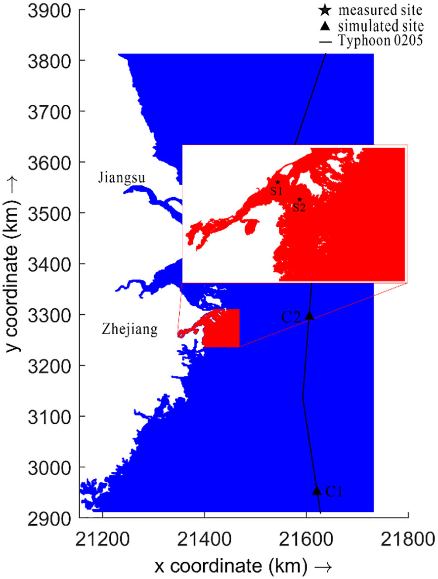
Figure 3 Computational model mesh, moving track of typhoon Rammasun, verification sites (S1, S2) and observation points (C1, C2).

3.3 Verification of astronomical tide

To verify the astronomical tide, the measured data collected from the S1 and S2 stations by SIO, during the period from June 1 to 13, 2002, were employed. The verification results are presented in Figure 4 and corresponding evaluation values are listed in Table 3. The RMSE values of the astronomical tide at S1 and S2 were determined to be 0.06m and 0.052m, indicating a small deviation between the simulated and measured values. The SS values for both stations were 0.98 and 0.99 denoting a high level of agreement between the simulation and measurement. These results establish a solid foundation for subsequent numerical simulations of storm tides.

FIGURE 4

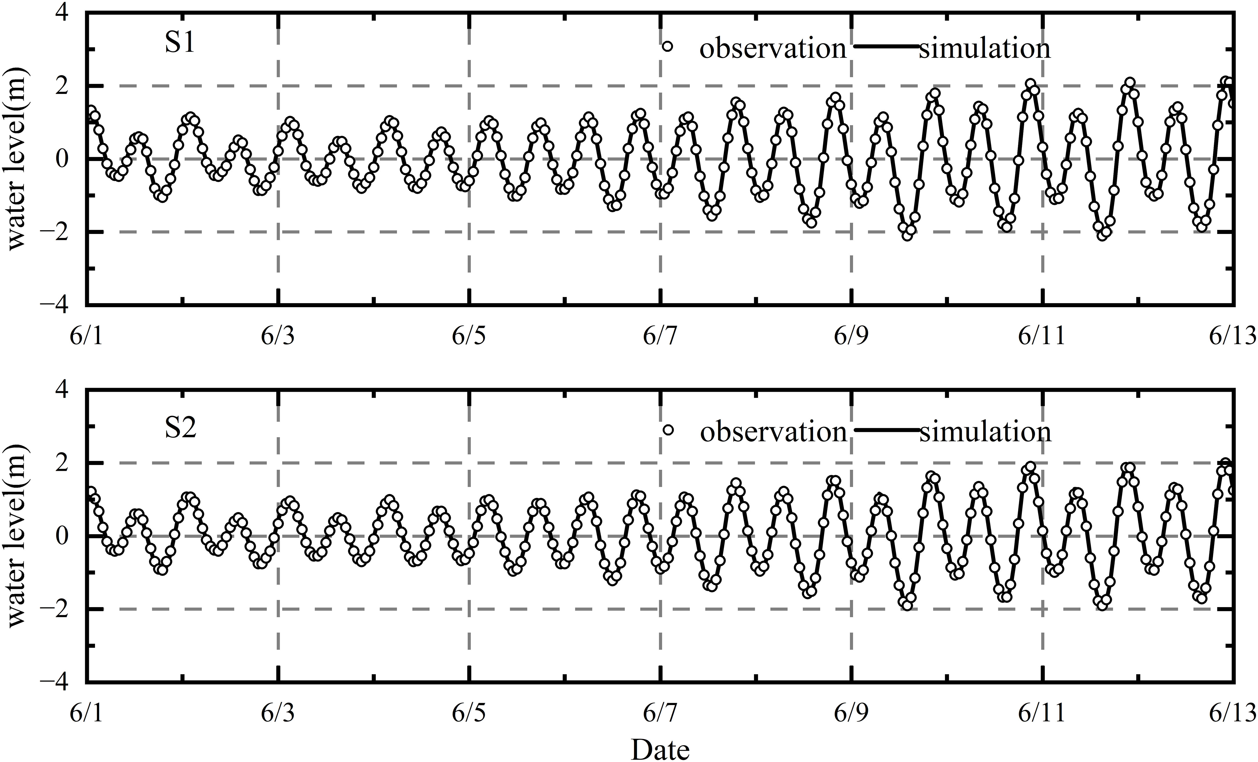
Figure 4 Verification of astronomical tide.

3.4 Verification of typhoon storm surge

In this study, we conducted a numerical simulation of typhoon storm tide during Typhoon Rammasun, employing the newly developed wind model to provide wind-stress input. The simulated water levels during the typhoon were compared with the measured values, as shown in Figure 5. The storm surge simulation driven by the new typhoon model exhibited a remarkable agreement with the observed data. Evaluation values for the present model are presented in Table 3, demonstrating its high accuracy. The SS values ranged from 0.98 to 0.99, while the RMSE values ranged from 0.14 to 0.19m.

FIGURE 5

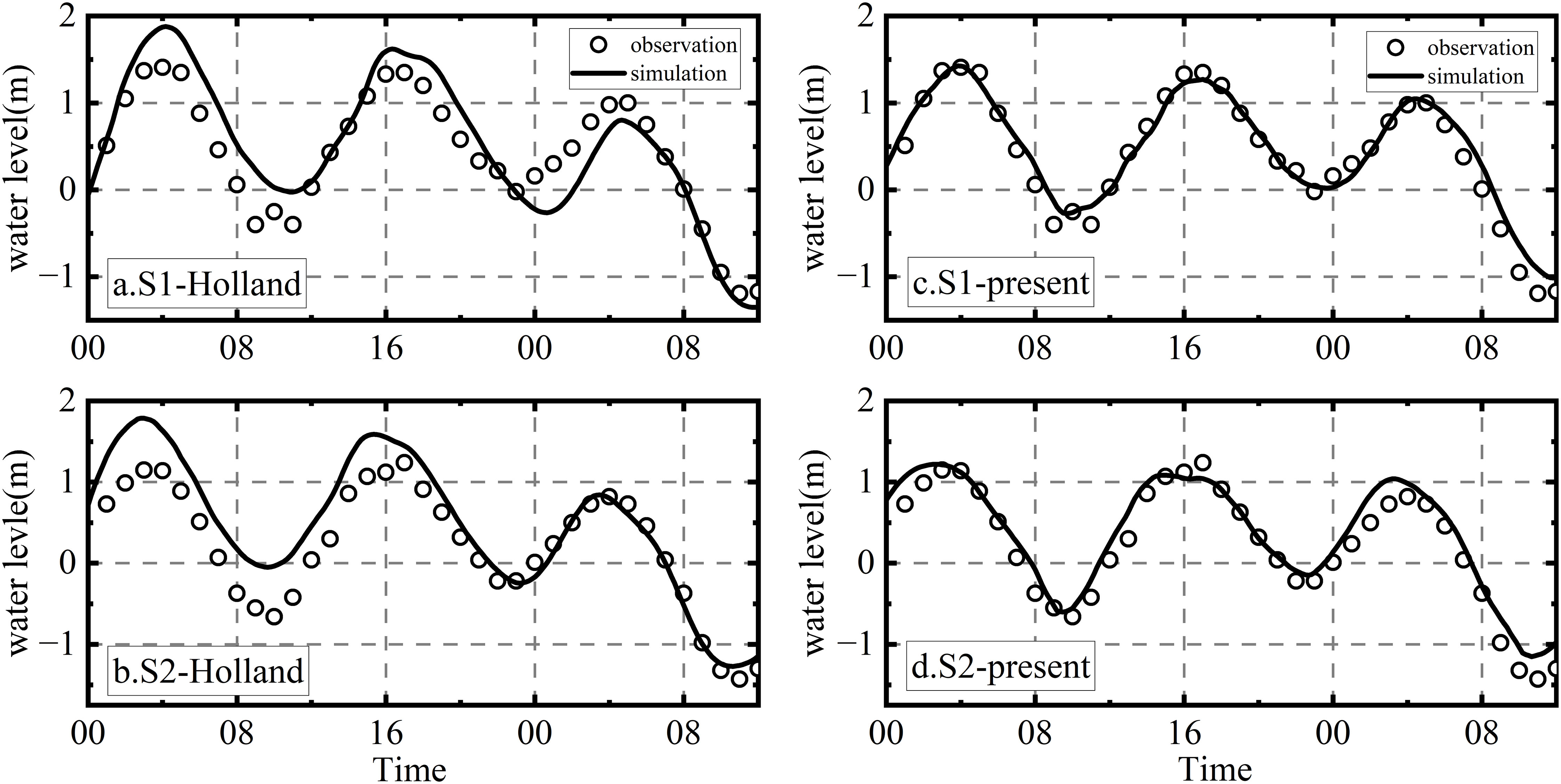
Figure 5 Verification of storm water level for the present and Holland model.

Figure 5 and Table 3 also show a comparison of the simulated storm surges based on the Holland model, along with the corresponding evaluation metrics. The results reveal that the simulations using the Holland model achieved a satisfactory performance, with RMSE values ranging from 0.31 to 0.36m and SS values of 0.95 to 0.96. However, they did not exhibit the same level of accuracy as the present model.

Overall, the numerical simulation results highlight the superior performance of the present model in accurately simulating typhoon storm surges during Typhoon Rammasun when compared to the Holland model.

3.5 Verification of SCV

In-situ measurements of SCV during typhoons are a particularly difficult and challenging task in severe weather conditions. Previous studies have primarily focused on storm surges or water levels, with limited attention given to SCVs (Liu and Huang, 2020; Li et al., 2022). To address this research gap, we collected valuable ADCP data on current velocity along a vertical line from 23:00 on July 3rd to 00:00 on July 6th, 2002, during Typhoon Rammasun. The data was obtained from SIO. We then verified the simulations of typhoon SCV using wind-stress inputs from the present model and the Holland model, as depicted in Figure 6 and Table 3.

FIGURE 6

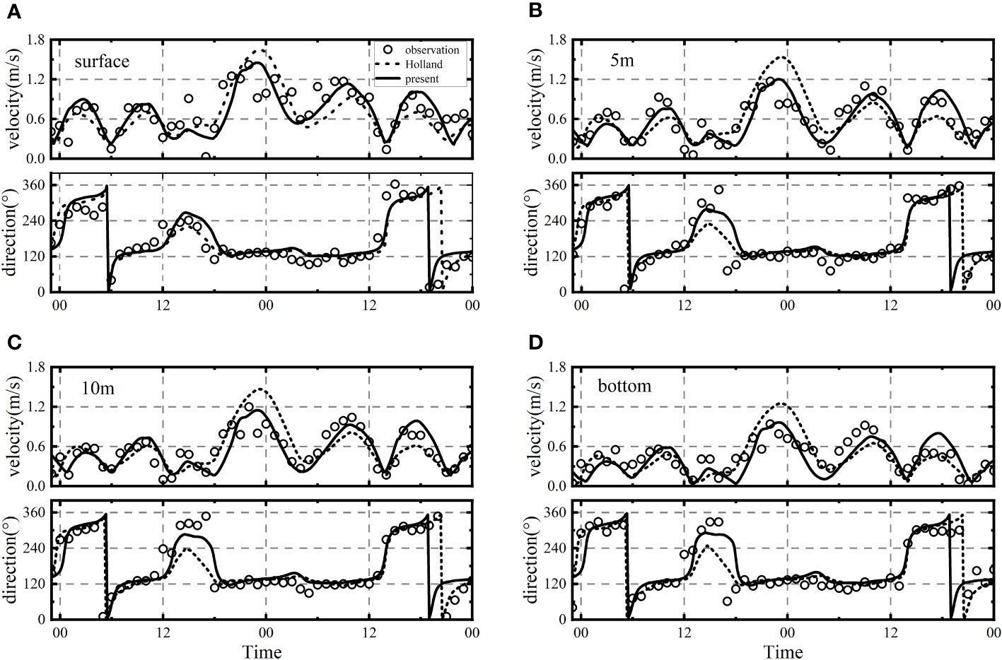
Figure 6 Verification of Typhoon SCVs for the present and Holland models. (A) Surface layer, (B) 5m layer, (C) 10m layer, (D) Bottom layer.

The measured data provided insights into the trend of typhoon SCV. Typhoon SCV exhibited a significant increase starting from 18:00 on July 4th, attributable to the influence of surface wind force, reaching its peak at 00:00 on July 5th. The maximum measured SCV gradually decreased from 1.5m/s at the surface to 0.9m/s at the bottom layer. Notably, the current direction changed from NW to SW between 12:00 and 18:00 on July 4th, with the surface direction exhibiting the most pronounced deflection. From 18:00 on the 4th to 12:00 on the 5th, the current directions across the entire depth ranged from WNW to ESE, influenced by the WNW wind, illustrating the significant impact of wind-stress during the typhoon.

Table 3 presents the SS and RMSE values for predicting SCVs using the two wind models compared with the measured data. Importantly, the present model outperformed the Holland model by a considerable margin. For example, at the surface and 5m layers, the present model achieved RMSE values of 0.15m/s and 0.11m/s, significantly lower than the corresponding 0.22m/s obtained with the Holland model. The SS values associated with the present model ranged from 0.89 to 0.96, while for the Holland model, they ranged from 0.83 to 0.87. These findings demonstrate the high accuracy and effectiveness of simulating SCVs using the present model. Notably, one of the key distinctions between the two models lies in the calculation of the maximum SCVs. The present model accurately predicted the maximum SCVs across the entire depth, whereas the Holland model overestimated these values by approximately 0.3 to 0.6m/s when compared with the measured data.

The overall accuracy of TSCV calculations was evaluated by using Mean Absolute Percentage Error (MAPE)

$\begin{array}{ll}MAPE=\frac{100\%}{N}{\displaystyle {\sum }_{i=1}^N\left|\frac{s_i-o_i}{o_i}\right|}& (25)\end{array}$

The results reveal that the present model performs better than Holland model. MAPE of the present model for the surface and 5m layers are 17.96% and 19.08%, while those of Holland model are 28.3% and 34.2%. Overall, the present model exhibits low error with MAPE of 24.11% and the error reduction of 27.6% compared to Holland model. The above-mentioned evidence proves convincingly that for predicting TSCV the new parametric wind model is superior to Holland model. These findings have important implications for improving the accuracy of oceanographic modeling and forecasting.

The findings from this study provide compelling evidence supporting the superiority of the present model over the Holland model. The MAPE of the present model for the surface and 5m layers are notably lower at 17.96% and 19.08% respectively, in contrast to the higher values of 28.3% and 34.2% obtained by the Holland model. In terms of overall performance, the present model demonstrates a remarkable low error with an MAPE of 24.11%, resulting in a substantial error reduction of 27.6% compared to the Holland model. These results highlight the clear advantages of the new parametric wind model in accurately predicting typhoon SCVs Table 3.

TABLE 3

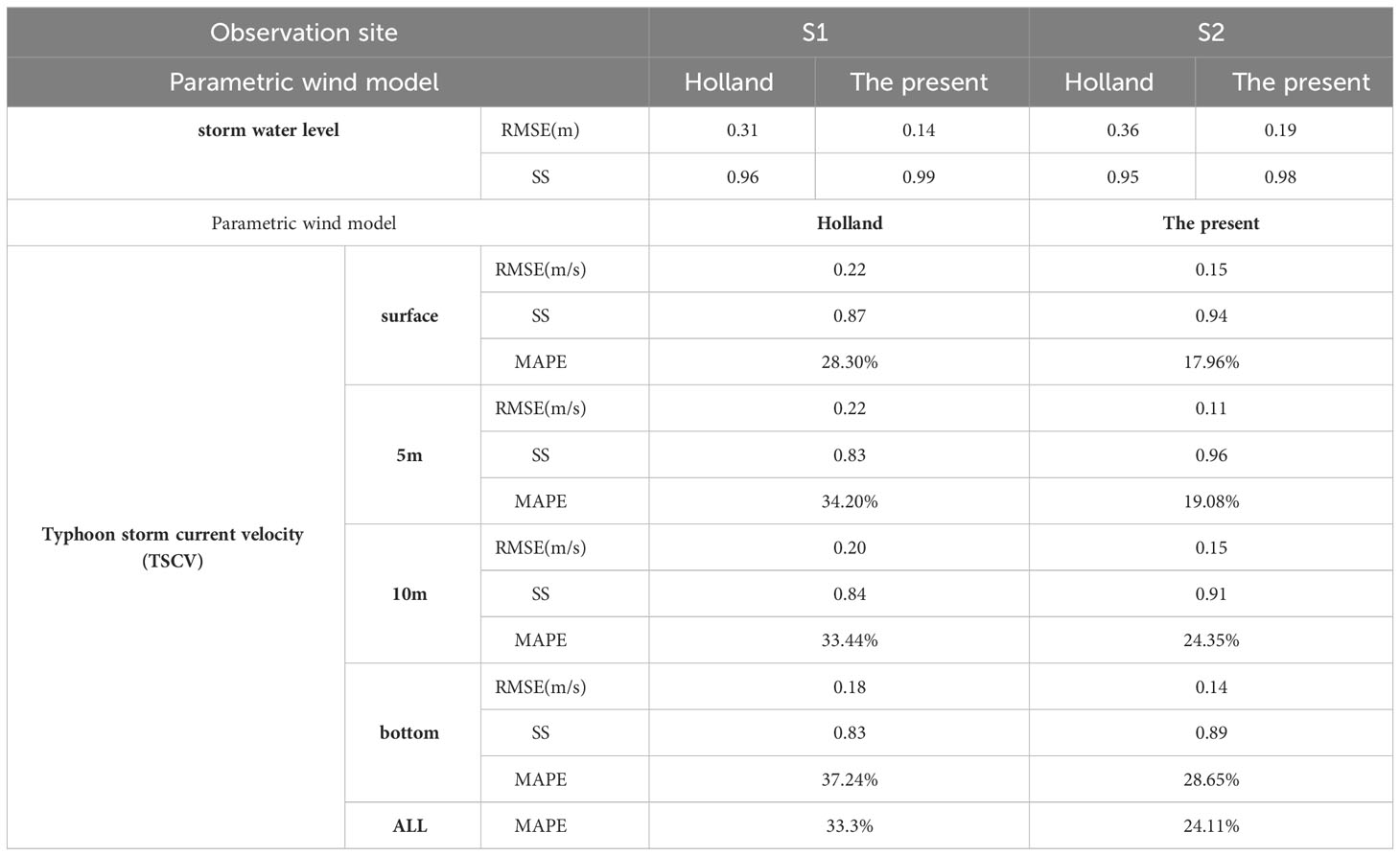
Table 3 Verification of storm water level and TSCV.

The implications of these findings are significant for enhancing the precision of oceanographic modeling and forecasting. By employing the present model, researchers and practitioners can achieve improved accuracy in predicting SCVs, which is crucial for understanding and mitigating the impacts of severe weather conditions. These advancements in modeling techniques hold promise for enhancing our understanding of ocean dynamics and supporting more effective decision-making in coastal management, disaster preparedness, and environmental conservation.

4 Analysis and discussions

4.1 Temporal variations of typhoon storm tides

Typhoon storm tides encompass both storm surges and current velocities, with the latter primarily influenced by wind speed. However, previous parametric models have struggled to provide accurate wind profiles, resulting in limited investigations into SCVs during typhoons/hurricanes. Furthermore, there has been a scarcity of measured data on SCVs during these extreme weather events. Thus, the analysis of SCVs can provide useful insights for coastal engineering.

The results of the calculations were analyzed at two specific points along the track of the typhoon, labelled C1 and C2, at a depth of approximately 140m (Figure 3). The temporal variations of pressure, water level, wind speed, and current velocity were examined and presented in Figure 7.

FIGURE 7

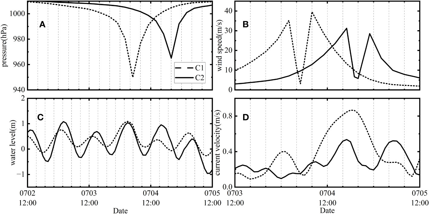
Figure 7 Temporal variations of typhoon storm tides driven by the present model. (A) pressure, (B) wind speed, (C) water level, (D) current velocity.

Figures 7A, B illustrate the temporal variations of pressure and wind speed at points C1 and C2. The minimum pressure was recorded at 950hPa and 965hPa as the typhoon center moved from C1 to C2. The wind speed displayed an “M-shape” pattern over time, with peak wind speeds of 35.2m/s observed when the northern radius of MW reached C1. Similarly, the minimum wind speeds occurred as the typhoon center moved towards C1. After an additional 3 hours, when the southern radius of MW reached C1, the peak wind speed reached 39.6m/s. Similar wind speed variations were observed at C2 as the typhoon progressed, albeit with a decrease in maximum wind speed correlated with the rise in central pressure.

Water level changes are primarily influenced by both the typhoon and tidal cycle. The fluctuations in water level corresponded to the 12.4-hour tidal cycle, with the maximum water level and significant surge occurring during the period of minimum pressure. The current velocity at C1, with a depth of 140m, increased to 0.4m/s when the first peak wind arrived. The minimum current velocity occurred shortly after the minimum wind. Subsequently, after a time lag of 10 hours from the second peak wind, the maximum current velocity reached 0.87m/s due to the ebb current aligning with the offshore wind. At C2, two peak velocities of 0.54m/s and 0.52m/s were observed. The maximum SCV at C2 was smaller than at C1 due to the inconsistent wind direction with the tidal current.

During typhoons, water levels generally correlate with pressure, while SCV is influenced not only by wind speed but also by the astronomical tidal current. Notably, the intensity of Typhoon SCV increases when its direction aligns with the astronomical tidal current, whereas it decreases when they oppose each other. These findings highlight the complex interplay between meteorological and tidal factors in shaping storm tides and SCV dynamics during typhoons.

4.2 The spatial distribution of storm tides around the typhoon center

Spatial variations in storm tides during typhoons are closely linked to the pressure and wind profiles. Figure 8 illustrates the spatial distributions of pressure, wind speed, water level, and current velocity within a 100 km radius from the typhoon center.

FIGURE 8

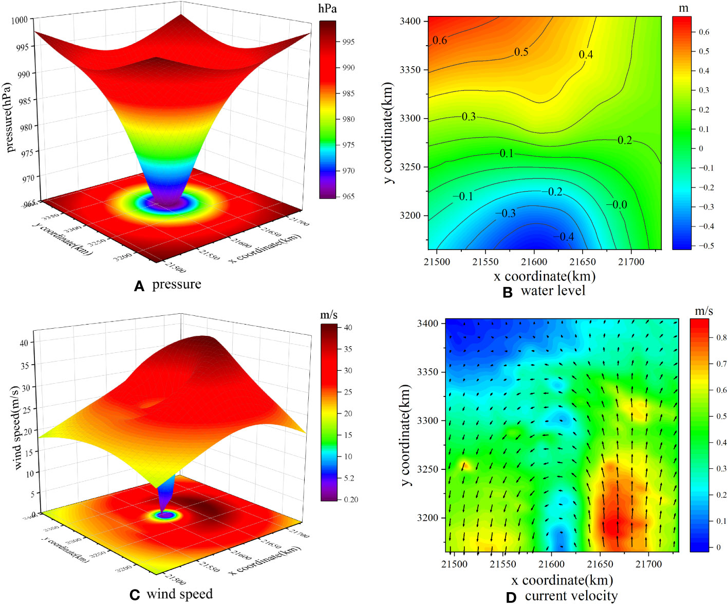
Figure 8 Spatial variations of typhoon and the corresponding storm tides driven by the present model. (A) pressure, (B) water level, (C) wind speed, (D) current velocity.

Figure 8A depicts the symmetrical pattern of pressure ranging from 965 to 998.7hPa. In Figure 8B, the contours of storm water level converge towards the typhoon center, a notable difference from the approximately parallel contours observed for tidal levels.

The 3D spatial distribution of wind speed during the typhoon exhibits an interesting asymmetrical funnel-shape, as presented in Figure 8C. On the right side along the typhoon’s moving direction, the MW is 20 m/s greater than on the left side. Additionally, within the typhoon’s eye, the wind speed on the right side exceeds that on the left by 10 m/s. This asymmetry in wind speed distribution has significant implications for the behavior of Typhoon SCVs.

Figure 8D shows that Typhoon SCVs, predominantly influenced by wind speed, rotate counterclockwise. The SCVs demonstrate a planar characteristic, with higher values observed at the east compared to the west. However, it is important to note that the spatial variation of SCVs lags behind that of the typhoon itself.

These spatial variations in pressure, wind speed, water level, and current velocity within the vicinity of the typhoon center shed light on the complex dynamics that govern storm tides during typhoons. The asymmetry in wind speed distribution and the influence of wind profiles on Typhoon SCVs highlight the intricate interplay between meteorological factors and their impact on storm surge dynamics. These findings contribute to a deeper understanding of the spatial behavior of storm tides and have important implications for typhoon forecasting and oceanographic modeling.

4.3 Nearshore storm current velocities

Typhoon storm tides pose significant risks to coastal infrastructure, including dikes, platforms, seabed pipelines, and cables. Understanding the characteristics of nearshore SCVs is therefore crucial, paralleling the importance of studying storm surges.

Figure 9 provides insight into the temporal variations of ACVs and SCVs within the nesting mesh during Typhoon Rammasun. At 20:00 on July 4th, ACVs in the open sea were relatively low, below 0.5m/s, and predominantly exhibited a northward direction. However, higher ACVs were observed within Xiangshan Bay and between the shoreline and the islands, peaking at 1.21m/s. After 4 hours, ACVs in the open sea remained below 0.5m/s, but their direction shifted southward. Subsequently, flood began at 4:00 the following day, causing tidal currents to flow into the bay, resulting in elevated velocities at the bay mouth, with a maximum of 1.34m/s.

FIGURE 9

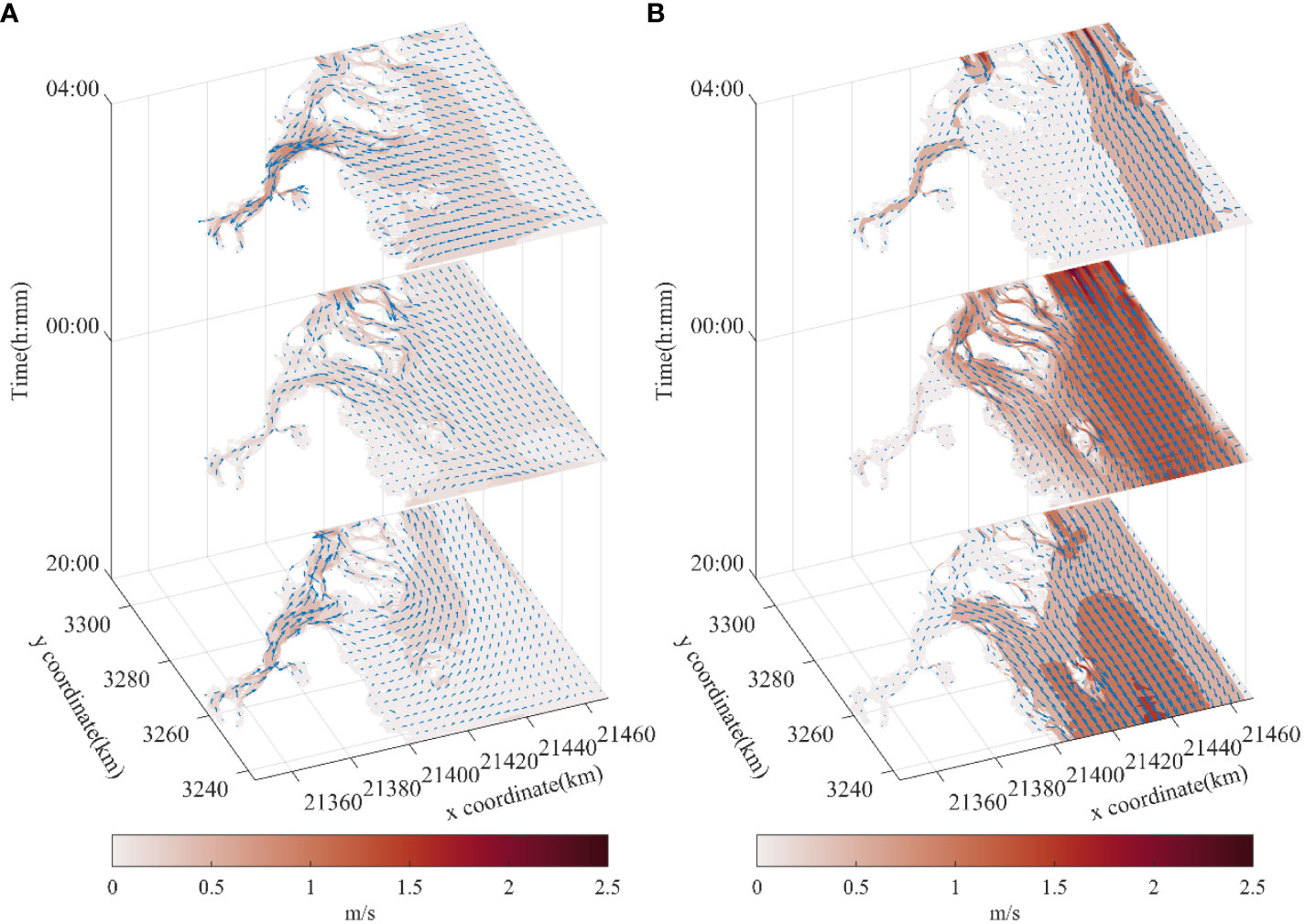
Figure 9 The current velocity field of astronomical tide and storm tide near the coast of Zhejiang. (A) astronomical tide current, (B) storm current.

The calculated Typhoon SCVs, driven by the present wind model, are depicted in Figure 9B. SCVs showed a significant increase, with a maximum velocity of 2.88m/s at 20:00 on the 4th. Notably, SCVs became almost negligible within the bay and waters between the shoreline and islands. However, after an additional 4 hours, SCVs exhibited a more noticeable increase, aligning with the ACVs that were consistent with the prevailing wind. By 4:00 on the 5th, ACVs were in opposition to the wind, leading to SCVs on the western sea being lower than ACVs, while the opposite was observed on the eastern side. However, near the coastlines on the northern side, SCVs exceeded 2.5m/s due to their alignment with the wind direction.

Unlike the one-dimensional nature of storm surges, SCVs introduce an additional dimension that necessitates consideration of both magnitude and direction. Typhoons exert significant influence on enhancing current velocities. Typically, ACV intensities in the open sea are relatively low, despite strong wind speeds, resulting in higher SCVs than ACVs. In coastal regions, particularly in bays, ACVs exhibit greater intensity. When the direction of ACVs contradicts the wind speed, the current velocity significantly diminishes. Conversely, when the two are aligned, it leads to destructive SCVs.

The maximum ACVs obtained from the small-scale model simulations are presented in Figure 10A. Notably, ACVs exceeding 1.5m/s were predominantly observed in Xiangshan Bay and the channels between islands, with the highest velocity reaching 2.6m/s. Figure 10B illustrates the maximum SCVs at each node. SCVs surpassing 2m/s were primarily distributed on the north side of Liuheng Island, the eastern sides of Taohua Island, and the Jiushan Islands, with the maximum velocity reaching 3.57m/s. It is noteworthy that SCVs in the open sea exhibited a significant increase, while those within Xiangshan Bay decreased.

FIGURE 10

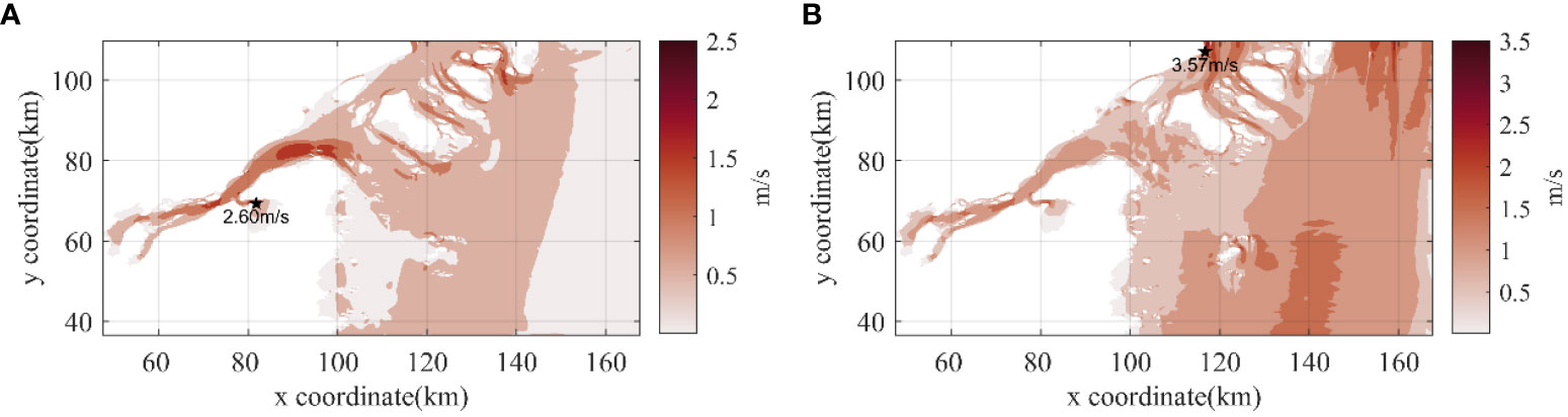
Figure 10 Spatial distribution of the maximum ACVs and SCVs. (A) maximum ACVs, (B) maximum SCVs.

Figure 11 displays the ratios of the maximum SCVs to ACVs. Ratios exceeding 3 were mainly concentrated in the eastern open sea and areas surrounding the islands, attributable to the substantial increase in SCVs influenced by typhoons. The highest ratio, reaching 16.9, was observed at the edge of an island. Importantly, the region where the ratios of maximum SCVs to ACVs exceeded 3 encompassed 21.4% of the entire computational domain.

FIGURE 11

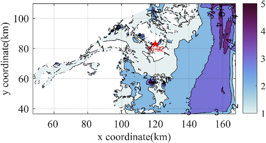
Figure 11 Ratios of SCVs to ACVs.

Understanding the dynamics of SCVs in conjunction with storm surges is crucial. By considering both magnitude and direction, these findings provide valuable insights into the spatial distribution of SCVs during typhoons. The study quantifies the ratios of SCVs to ACVs, shedding light on the impact of typhoons on current intensification, particularly in regions where the ratio exceeds a threshold of 3. This knowledge enhances our understanding of nearshore current dynamics during extreme weather events, aiding in coastal planning, hazard mitigation, and the protection of vulnerable coastal infrastructure.

5 Conclusions

Key findings of this study are as follows:

1. A new typhoon wind field model incorporating sea surface resistance was developed, demonstrating high accuracy and improved performance compared to existing models. Wind speed predictions from the new model aligned well with measured data for hurricanes and typhoons, exhibiting a skill score of 0.94-0.99. The new model outperformed Holland and Fujita-Takahashi models in wind speed calculation, showcasing lower root mean square error (RMSE) during hurricanes/typhoons. The new model significantly advances the accuracy of typhoon wind speed estimation.

2. A numerical model for typhoon storm tides, incorporating wind stress calculated from the new model, produced excellent agreement between predicted and measured storm surges at two sites (skill scores of 0.98 and 0.99). While storm surges calculated using the Holland model also showed reasonable agreement with observations, they were not as accurate as the present model.

3. Simulation of storm current velocities (SCVs) and comparison with ADCP measured data during typhoon Rammasun at S2 station revealed that the new model, driven by wind stress, exhibited skill scores of 0.89-0.96 and a mean absolute percentage error (MAPE) of 24.11% compared to observations. In contrast, SCVs driven by the Holland model had an MAPE of 33.3%. The new model demonstrated substantial improvement in SCV estimation over the Holland model and holds great potential for oceanographic modeling and forecasting.

4. Typhoon storm surges are primarily influenced by pressure, while SCVs are influenced by wind speed in open sea. The peak water level corresponds approximately to the minimum pressure. SCVs near the typhoon’s maximum wind (MW) radius exhibit a counterclockwise rotation and are generally consistent with wind speed, although the occurrence of maximum SCV lags behind that of the MW in both time and space.

5. Typhoons significantly enhance SCVs, with SCV values surpassing those of astronomical tidal current velocities (ACVs) in open seas where ACVs are relatively low. When ACV directions align with the wind, SCVs experience significant increases, while opposite directions lead to substantial SCV reduction. The maximum SCV recorded was 3.57m/s, and regions with SCV to ACV ratios exceeding 3 accounted for 21.4% of the study area.

Data availability statement

The raw data supporting the conclusions of this article will be made available by the authors, without undue reservation.

Author contributions

ZS: Conceptualization, Funding acquisition, Methodology, Resources, Supervision, Writing – review & editing. KD: Data curation, Formal Analysis, Methodology, Validation, Visualization, Writing – original draft, Writing – review & editing, Conceptualization, Investigation. ZL: Investigation, Validation, Writing – review & editing. FC: Data curation, Investigation, Writing – review & editing. SZ: Conceptualization, Investigation, Writing – original draft.

Funding

This work was supported by Major Project of Science and Technology in Zhejiang Province (No.2023C03119) and Key Program form Natural Science Foundation of China (No.91647209).

Conflict of interest

The authors declare that the research was conducted in the absence of any commercial or financial relationships that could be construed as a potential conflict of interest.

Publisher’s note

All claims expressed in this article are solely those of the authors and do not necessarily represent those of their affiliated organizations, or those of the publisher, the editors and the reviewers. Any product that may be evaluated in this article, or claim that may be made by its manufacturer, is not guaranteed or endorsed by the publisher.

References

Brenner S., Gertman I., Murashkovsky A. (2007). Preoperational ocean forecasting in the southeastern Mediterranean Sea: Implementation and evaluation of the models and selection of the atmospheric forcing. J. Mar. Syst. 65, 268–287. doi: 10.1016/j.jmarsys.2005.11.018

CrossRef Full Text | Google Scholar

Çalışır E., Soran M. B., Akpınar A. (2021). Quality of the ERA5 and CFSR winds and their contribution to wave modelling performance in a semi-closed sea. J. OPER OCEANOGR 0, 1–25. doi: 10.1080/1755876X.2021.1911126

CrossRef Full Text | Google Scholar

Carvalho D. (2019). An assessment of NASA’s GMAO MERRA-2 reanalysis surface winds. J. Clim. 32, 8261–8281. doi: 10.1175/JCLI-D-19-0199.1

CrossRef Full Text | Google Scholar

Chan J. C. L. (2007). Decadal variations of intense typhoon occurrence in the western North Pacific. P ROY Soc. A-MATH PHY 464, 249–272. doi: 10.1098/rspa.2007.0183

CrossRef Full Text | Google Scholar

Chan J. C. L., Liu K. S. (2004). Global warming and Western North Pacific typhoon activity from an observational perspective. J. Clim. 17, 4590–4602. doi: 10.1175/3240.1

CrossRef Full Text | Google Scholar

Director of Meteorology (1977). Report on cyclone Tracy, december 1974 (Canberra, Australia: Australian Government Publication Service).

Google Scholar

Director of Meteorology (1979). Report on cyclone Joan, december 1978 (Melbourne, Australia: Bureau of Meteorology, DSE).

Google Scholar

Dullaart J. C. M., Muis S., Bloemendaal N., Aerts J. C. J. H. (2020). Advancing global storm surge modelling using the new ERA5 climate reanalysis. Clim. Dyn. 54, 1007–1021. doi: 10.1007/s00382-019-05044-0

CrossRef Full Text | Google Scholar

Holland G. J. (1980). An analytic model of the wind and pressure profiles in hurricanes. Mon Weather Rev. 108, 1212–1218. doi: 10.1175/1520-0493(1980)108<1212:AAMOTW>2.0.CO;2

CrossRef Full Text | Google Scholar

Jelesnianski C. P. (1965). A numerical calculation of storm tides induced by a tropical storm impinging on a continental shelf. Monthly Weather Rev. 93, 343–358. doi: 10.1175/1520-0493(1993)093<0343:ANCOS>2.3.CO;2

CrossRef Full Text | Google Scholar

Karim M. F., Mimura N. (2008). Impacts of climate change and sea-level rise on cyclonic storm surge floods in Bangladesh. Glob Environ. Change 18, 490–500. doi: 10.1016/j.gloenvcha.2008.05.002

CrossRef Full Text | Google Scholar

Li L., Li Z., He Z., Yu Z., Ren Y. (2022)Investigation of storm tides induced by super typhoon in macro-tidal Hangzhou Bay (Accessed April 4, 2023).

Google Scholar

Lin N., Chavas D. (2012). On hurricane parametric wind and applications in storm surge modeling. J. GEOPHYS RES-ATMOS 117, D09120. doi: 10.1029/2011JD017126

CrossRef Full Text | Google Scholar

Liu W.-C., Huang W.-C. (2020). Investigating typhoon-induced storm surge and waves in the coast of Taiwan using an integrally-coupled tide-surge-wave model. Ocean Eng. 212, 107571. doi: 10.1016/j.oceaneng.2020.107571

CrossRef Full Text | Google Scholar

Ramos Valle A. N., Curchitser E. N., Bruyere C. L., Fossell K. R. (2018). Simulating storm surge impacts with a coupled atmosphere-inundation model with varying meteorological forcing. J. Mar. Sci. Eng. 6, 35. doi: 10.3390/jmse6020035

CrossRef Full Text | Google Scholar

Roelvink J. A., Van Banning G. (1995). Design and development of DELFT3D and application to coastal morphodynamics. Oceanogr. Lit. 11, 925.

Google Scholar

Sun Z. L., Huang S. J., Nie H., Jiao J. G., Huang S. H., Zhu L. L., et al. (2015). Risk analysis of seawall overflowed by storm surge during super typhoon. Ocean Eng. 107, 178–185. doi: 10.1016/j.oceaneng.2015.07.041

CrossRef Full Text | Google Scholar

Sun Z., Zhong S. (2018). Simulation and analysis of storm surge at Zhoushan fishing port. Haiyang Xuebao 2020, 136–143. doi: 10.3969/j.issn.0253-4193.2020.01.014

CrossRef Full Text | Google Scholar

Torres M. J., Hashemi M. R., Hayward S., Spaulding M., Ginis I., Grilli S. T. (2019). Role of hurricane wind models in accurate simulation of storm surge and waves. J. WATERW PORT Coast. 145, 04018039. doi: 10.1061/(ASCE)WW.1943-5460.0000496

CrossRef Full Text | Google Scholar

Ueno T. (1966). Non-linear numerical studies on tides and surges in the central part of Seto Inland Sea. Oceanogr. Mag. 16 (2), 53–124.

Google Scholar

Vijayan L., Huang W., Yin K., Ozguven E., Burns S., Ghorbanzadeh M. (2021). Evaluation of parametric wind models for more accurate modeling of storm surge: a case study of Hurricane Michael. Nat. Hazards (Dordr) 106, 2003–2024. doi: 10.1007/s11069-021-04525-y

CrossRef Full Text | Google Scholar

Wang X., Yin Q., Zhang B. (1991). Research and application of a forecasting model of typhoon surges in China seas. Adv. Water Sci. 2, 1–10. doi: 10.3321/j.issn:1001-6791.1991.01.001

CrossRef Full Text | Google Scholar

Woodruff J. D., Irish J. L., Camargo S. J. (2013). Coastal flooding by tropical cyclones and sea-level rise. Nature 504, 44–52. doi: 10.1038/nature12855

PubMed Abstract | CrossRef Full Text | Google Scholar

Wu J. (1982). Wind-stress coefficients over sea surface from breeze to hurricane. J. Geophys. Res. 87, 9704–9706. doi: 10.1029/JC087iC12p09704

CrossRef Full Text | Google Scholar

Wu L., Wang B., Geng S. (2005). Growing typhoon influence on east Asia. Geophys. Res. Lett. 32, L18703. doi: 10.1029/2005GL022937

CrossRef Full Text | Google Scholar

Zhang H., Sheng J. (2015). Examination of extreme sea levels due to storm surges and tides over the northwest Pacific Ocean. Cont Shelf Res. 93, 81–97. doi: 10.1016/j.csr.2014.12.001

CrossRef Full Text | Google Scholar