Motor imagery electroencephalogram classification algorithm based on joint features in the spatial and frequency domains and instance transfer

1. Introduction

In recent years, brain-computer interface (BCI) systems have attracted great attention because they can provide another communication channel for people who have lost independent motor ability by decoding neural signals (Wolpaw et al., 2002). This system converts electroencephalography (EEG) collected from the scalp into control commands for computers or other external devices, thereby achieving direct interaction between the brain and external devices (Xu et al., 2018). In EEG-based BCI experiments, motor imagery (MI) is a commonly used task paradigm.

Brain-computer interface based on MI means that there is no actual physical behavior involved, but rather the thoughts in the brain are used to imagine bodily movements, which are then translated into actual operations through a controller. MI activates brain regions that are similar to those activated during actual physical movement (Holmes and Calmels, 2008; Miltona et al., 2008), which can promote the repair or reconstruction of damaged motor pathways, has great application value in the field of rehabilitation. However, due to the small amount of Mi-EEG sample data of a single subject and the large individual differences among different subjects (Manali et al., 2020), the classification model has low accuracy and poor generalization ability in the MI classification task.

To solve these problems, researchers have conducted extensive studies. Due to the asymmetric energy differences in the human spatial brain area during motor imagery, researchers usually use the Common Spatial Pattern (CSP) algorithm to extract distinguishable spatial features from multi-channel EEG signals (Ramoser et al., 2000; Amirhossein et al., 2016). In addition, EEG signals are mainly rhythmic signals, and Event-Related Desynchronization (ERD) (Zhang et al., 2021) and Event-Related Synchronization (ERS) (Bastien et al., 2020) occur within specific frequency bands. At the same time, the CSP algorithm directly filters spatially in the frequency domain, so frequency domain information cannot be ignored for MI classification. Therefore, many scholars have proposed combining spatial and frequency domain features to fully explore EEG and enrich EEG features. For example, Ai et al. (2019) used the CSP algorithm and the local characteristic-scale decomposition (LCD) algorithm to extract spatial and frequency domain features, respectively, and combined the two types of features. Finally, they used the Spectral Regression Discriminant Analysis (SRDA) classifier for classification, achieving an average classification accuracy of 74.5%. However, this method ignores the personalized differences between subjects, resulting in poor generalization ability of the classification model.

In recent years, studies have shown that transfer learning can improve model performance in target tasks by learning and transferring information from source tasks (Feng et al., 2022). Therefore, some researchers hope to reduce the individual differences among different subjects through transfer learning (Cao et al., 2021; Feng et al., 2023), so as to improve the performance of the classification model. For example, He and Wu (2019) proposed a weighted logistic regression transfer learning algorithm based on Euclidean Space (EA), which aligns the EEG data of the source domain and target domain in the data preprocessing stage to reduce the differences between signals. In the feature extraction stage, the CSP algorithm is used to extract the feature values of different subjects, and then the Kullback-Leibler (KL) divergence of these feature values is calculated. Finally, the KL is used to adjust the Linear Discriminant Analysis (LDA) of the transfer learning for classification, achieving an average classification accuracy of 73.5%. However, this EA-CSP-LDA algorithm is not sensitive enough to non-linear data, resulting in poor classification performance. In addition, Zhou and Tian (2021) proposed a transfer multi-layers convolutional neural networks (TMCNN) algorithm, which first constructs a transfer network model capable of learning a large number of common features of the source domain, and then connects convolutional-pooling blocks to form four convolutional network structures with different depths. These structures are parallelly fused as a multi-level fusion feature extractor, and finally classified to achieve an average classification accuracy of 80.9%. However, this algorithm requires a large amount of data for model training, and the model is prone to overfitting when the dataset is small.

Due to the limited generalization ability of a single classifier, it is easy to overfit, so some researchers proposed to use ensemble learning to construct classifier. For example, Li et al. (2011) used a BP neural network as a weak classifier under the AdaBoost ensemble learning framework to form the BP-AdaBoost basic network classifier model. The model first extracts EEG features based on the Hilbert-Huang transform, and then introduces a forgetting factor to improve the AdaBoost algorithm, enhancing its temporal correlation by changing the initial weights of the samples. Finally, the BP neural network is used as a weak classifier and integrated into the BP-AdaBoost classifier. This model improves the classification accuracy by 23.42% compared to the traditional BP neural network, and achieves an average classification accuracy of 81.1%. However, the training time of BP neural network is long and it is prone to getting stuck in local optimal solutions, leading to a decrease in the performance of the classifier.

Inspired by the above studies, in order to break through the limitations of single domain EEG features to varying degrees, provide more comprehensive and detailed EEG analysis, and to simultaneously reduce the impact of small sample sizes of MI-EEG samples from individual subjects and inter-individual differences across subjects on MI task classification models, this paper proposes an EEG joint feature classification algorithm based on instance transfer and ensemble learning. The algorithm includes three stages: the first stage is preprocessing of source and target domain data; the second stage is to use the CSP algorithm and Power Spectral Density (PSD) to extract spatial and frequency domain features, respectively, and to combine the two features as EEG joint features, so as to fully explore EEG and enrich EEG features, and improve MI identification performance (Bin et al., 2019; Qiu et al., 2022); The third stage is to classify MI-EEG using an ensemble learning algorithm based on kernel mean matching (KMM) (Xing et al., 2007) and adaptive enhancement of transfer learning (TrAdaBoost) (Dai et al., 2007). Firstly, the KMM algorithm is used to adjust the sample weights to make the feature distribution of the source domain closer to that of the target domain. Then, the obtained weight sample matrix is used as the initialization weight matrix of the TrAdaBoost algorithm to initialize the training samples. Next, several weak classifiers are trained by using the initialized training sample data, and finally a strong classifier is integrated by weighted voting strategy. The algorithm makes full use of the EEG joint features and eliminates the individual differences of different subjects as much as possible. Repeated validation and testing show that the proposed algorithm can improve the classification performance of MI-EEG.

2. Materials and preprocessing

2.1. Data description

The MI-EEG data used in this paper is obtained from BCI Competition IV Dataset 2a and BCI Competition IV Dataset 2b (Tangermann et al., 2012).

The BCI Competition IV Dataset 2a is a dataset that collected EEG signals from 22 electrodes and recorded the locations of three electrooculogram (EOG) scalp electrodes for nine subjects. During the experiment, the subjects were asked to perform four different motor imagery tasks involving the left hand, right hand, foot, and tongue. Subjects sat in a comfortable chair and completed sessions consisting of six runs, with 48 motor imagery trials per run. In total, each session had 288 trials, with 72 trials performed for each type of motor imagery task.

The BCI Competition IV Dataset 2b is a dataset that collected EEG signals from three electrodes (C3, Cz, and C4) and recorded the locations of three EOG scalp electrodes for nine subjects. During the experiment, the subjects were asked to perform two different motor imagery tasks involving the left hand and right hand. Subjects sat in a comfortable chair and completed sessions consisting of six runs, with 20 motor imagery trials per run. In total, each session had 120 trials, with 60 trials performed for each type of motor imagery task.

This study only used data from motor imagery tasks involving the left and right hands. Prior to the start of each session, a 5 min EOG recording was performed to eliminate the influence of eye movement artifacts, followed by the start of the run. During each trial, subjects were required to fixate on the screen for 2 s before engaging in 4 s of motor imagery. The timing scheme of one session is shown in Figure 1, and the timing scheme of the experimental paradigm is shown in Figure 2. In addition, a sampling frequency of 250 Hz and a bandpass and a bandpass filter of 0.5–100 Hz were used during the experiment, along with a sensitive amplifier of 100 μV and a 50 Hz notch filter.

FIGURE 1

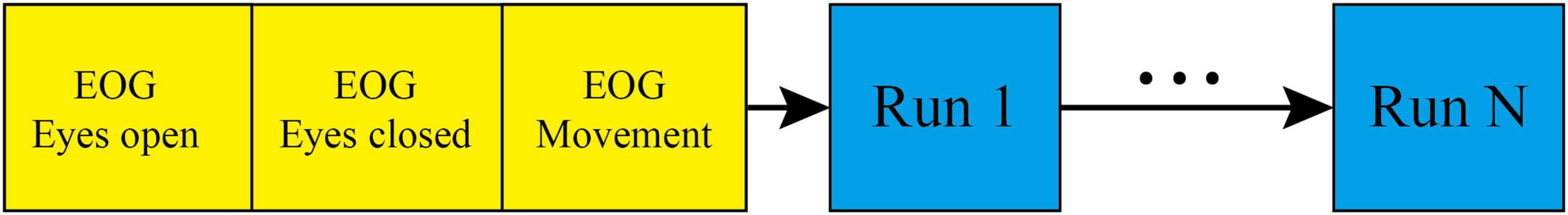
Figure 1. Timing scheme of one session.

FIGURE 2

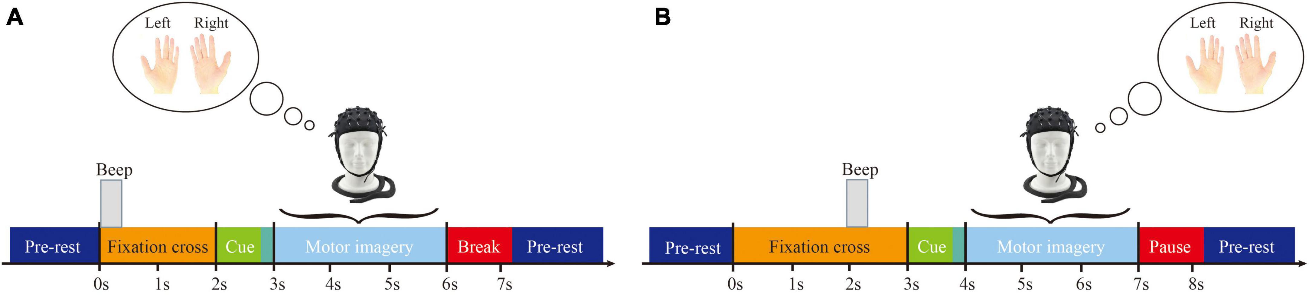
Figure 2. Timing scheme of the experimental paradigm. (A) Dataset 2a. (B) Dataset 2b.

In the experiment, a total of 22 scalp electrodes based on the international 10–20 system were used, including Fz, FC3, FC1, FCz, FC2, FC4, C5, C3, C1, Cz, C2, C4, C6, CP3, CP1, CPz, CP2, CP4, P1, Pz, P2, and POz, left mastoid reference, right mastoid grounding, as shown in Figure 3A. In addition, three EOG electrodes were used, as shown in Figure 3B.

FIGURE 3

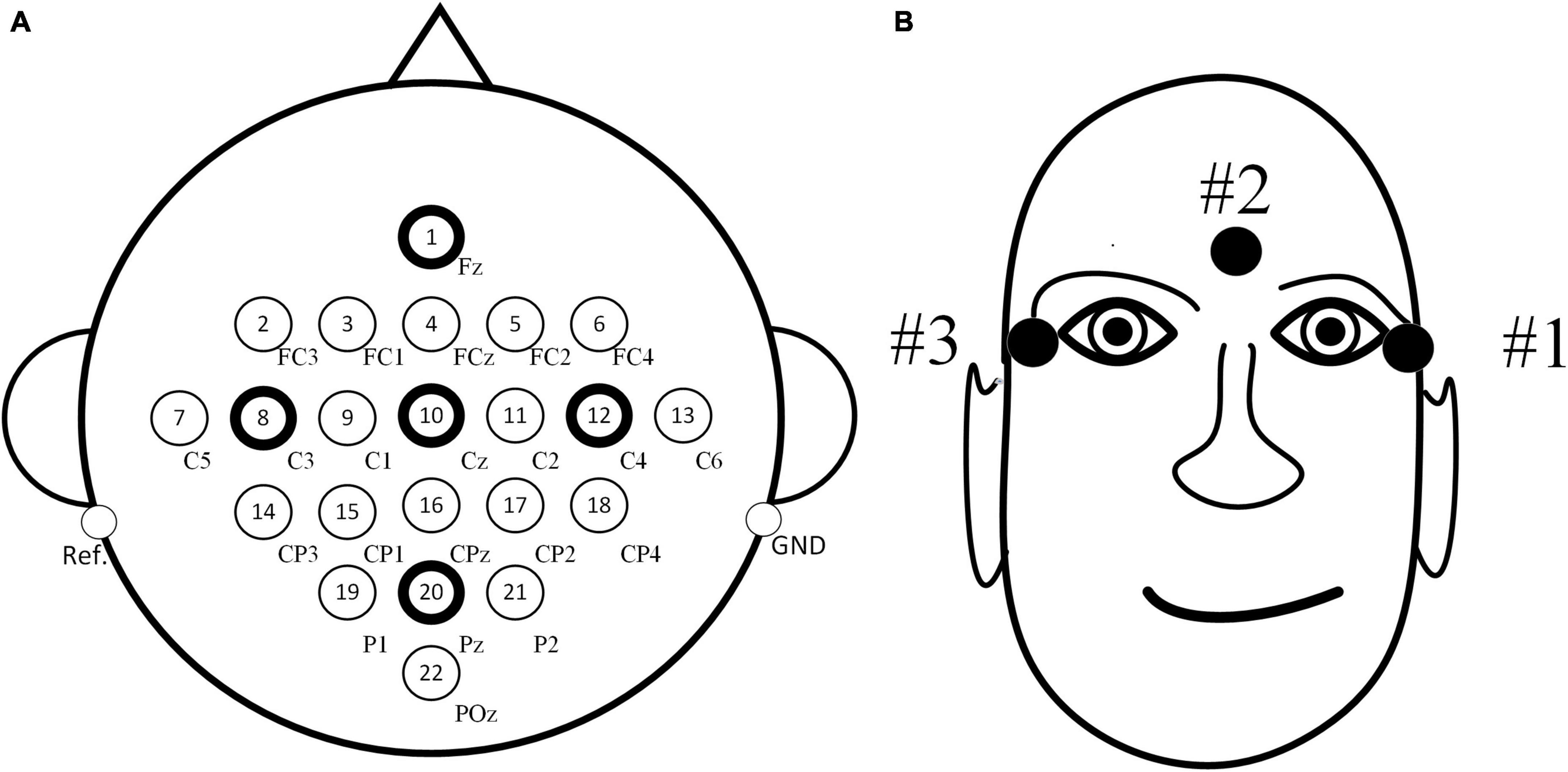
Figure 3. Distribution maps of electrode positions. (A) Positions of electroencephalography (EEG) electrodes. (B) Positions of electrooculogram (EOG) electrodes.

2.2. Data preprocessing

In the data preprocessing process of this study, the main steps used include channel selection, bandpass filtering, and time window processing. The detailed operation is as follows: In the channel selection step, the data recorded from the three EOG channels need to be removed, and the remaining EEG channels are used. As the relevant rhythmic signals during motor imagery are divided into μ rhythm signal of 8–12 Hz and β rhythm signal of 13–30 Hz (Chen et al., 2022), in the bandpass filtering step, a bandpass filter of 8–30 Hz is used to filter the selected EEG to improve the signal-to-noise ratio. Based on the experimental paradigm, each trial includes 4 s of motor imagery task time. Additionally, in the time window processing step, EEG corresponding to the motor imagery task time of 0.5–3.5 s after the cue are extracted, so as to better adapt to the needs of subsequent analysis by using the corresponding data from the 3 s time window in each trial, and improve the efficiency of data processing. The data preprocessing workflow is illustrated in Figure 4.

FIGURE 4

Figure 4. Data preprocessing workflow.

3. Related work

3.1. Spatial-frequency joint feature extraction

In order to fully explore MI-EEG signals and enrich EEG features, it is necessary to use multiple feature extraction methods to extract various types of features. This study used the CSP algorithm and PSD algorithm to extract spatial domain features and frequency domain features, respectively, and combined the two features as EEG joint features to provide more detailed and accurate EEG features, which could offer more comprehensive data support for subsequent signal processing and analysis.

3.1.1. Spatial domain feature extraction based on CSP

common space mode is an algorithm for spatial filtering feature extraction that is extensively applied to binary classification MI-EEG tasks. It takes advantage of the characteristic of asymmetric energy differences in spatial brain areas during motor imagery, and projects the two types of EEG onto a subspace to decompose them into different spatial patterns. The fundamental principle of CSP algorithm involves diagonalization of matrices to obtain an optimal set of spatial filters, and then project the feature matrix to maximize the difference in variance between the two types of signals. This ultimately extracts spatial feature vectors with high discrimination ability, making it suitable for distinguishing between two types of MI tasks. The main process is shown in Figure 5.

FIGURE 5

Figure 5. Common Spatial Pattern (CSP) feature extraction process.

(1) Sorting and segmenting the preprocessed data._{FN=[f1(t),f2(t),…,fk(t),]^T} represents the signal of experiment _N, with _k electrodes and _n trials per experiment. _Trace(.) is used to solve the matrix rank. The mixed-space covariance matrix _Hc is calculated as follows:

$H_c=\frac{1}{n}(\sum \frac{(F_1{F}_1^T)}{\text{trace}(F_1{F}_1^T)}+\sum \frac{(F_2{F}_2^T)}{\text{trace}(F_2{F}_2^T)})(1)$

(2) The mixed covariance space matrix _Hc is subjected to orthogonal whitening transformation, where I. represents the identity matrix, to obtain the whitened matrix _R that satisfies the following condition.

$R{H}_c{R}^T=I(2)$

(3) Performing Singular Value Decomposition (SVD) on eigenvalue _{C1, C2} with _{C1=RH1R^T , C2=RH2R^T} ,yields the diagonal matrix _P and the orthogonal matrix _Q:

$C_j=Q{P}_j{Q}^T\mathit{\hspace{1em}\hspace{1em}\hspace{1em}\hspace{1em}\hspace{0.5em} }(j=1,\mathrm{\hspace{0.33em}2})(3)$

(4) As inferred from (3), _{I=C1+C2, P2=I–P1}. When any element in _Cj approaches _I, the other elements of _Cj will approach the zero matrix. This maximizes the variance differences between the two classes of signals. Therefore, the spatial filtering _Z of the N-th EEG is:

$Z=Q^{T}Q{F}_N(4)$

(5) Spatial feature _fj of MI-EEG:

$f_j=\frac{var(Z_j)}{{\sum }_{j=1}^{m}var(Z_j)}(5)$

Among them, _Zj is the projection of _FN onto the spatial filter, _m is the number of selected feature parameters, _f is the feature value. _Var(.) is the variance of the matrix.

3.1.2. Frequency domain feature extraction based on PSD

As the EEG are non-stationary random signals, this study used the Welch method (Bin et al., 2019) in the PSD algorithm to extract frequency domain features from the EEG. This method reduces the random fluctuations in signals to obtain results with smaller variance and smoother curves, aiming to extract high-discriminative frequency domain features. The algorithm involves segmenting complex signals, applying window functions to calculate power spectral density, and finally outputting the averaged results. The main process is illustrated in Figure 6.

FIGURE 6

Figure 6. Power spectral density (PSD) feature extraction process.

(1) Segment the EEG _{f(m), m=0, 1, …, K–1} into _R segments, each containing _Ndata points, where the length of the EEG is _K. Segment _j of data can be represented as:

$f_j(m)=f(jN-N+n),0\le j\le R,0\le m\le N(6)$

(2) Apply a windowing function _w(m) to each segment of data, and then normalize the resulting periodogram _P(λ).

$P(\mathrm{\lambda })=\frac{1}{NU}{\left|\sum _{m=0}^{N-1}{f}_j(m)w(m)e^{-i2\mathrm{\pi }\mathrm{\lambda }}\right|}^2,j=1,\mathrm{\hspace{0.33em}2},\mathrm{\dots },N-1(7)$

(3) The final estimate of power spectral density _Pwelch(λ) is:

$P_{welch}(\mathrm{\lambda })=\frac{1}{R}\sum _{j=1}^{R}P(\mathrm{\lambda })(8)$

Where _Uis the normalization factor, _λ is the frequency, _P(λ) is the normalized periodogram, and _Pwelch(λ) is the power spectral density.

3.2. Ensemble learning classification

In this study, an ensemble learning algorithm based on KMM and TrAdaBoost (K-T) was used to classify MI-EEG. First, the sample weight matrix obtained by the KMM algorithm was used as the initial sample weight matrix for the TrAdaBoost algorithm. Then, several weak classifiers were trained using the initialized training samples. Finally, a strong classifier was obtained using a weighted voting strategy.

3.2.1. KMM algorithm

Due to individual differences, different subjects may have different feature distributions in their EEG. KMM can adjust the sample weights to make the feature distribution of the source domain similar to that of the target domain. Firstly, the raw feature Space was mapped to Reproducing Kernel Hilbert Space (RKHS) (Gertton et al., 2012), and then the mean difference between the source domain samples and the target domain samples in the RKHS was computed, resulting in a set of weight parameter matrices. These matrices can be used to re-assign weights to the training samples, aiming to achieve the feature distribution of the source domain approaching that of the target domain under the action of the nuclear space. The process can be expressed as follows:

$min{||\frac{1}{n}\sum _{i=1}^n{\mathrm{\beta }}_i\mathrm{\Phi }\left(x_i^s\right)-\frac{1}{m}\sum _{i=1}^m\mathrm{\Phi }\left(x_i^t\right)||}_H^2(9)$

Where,$x_i^s$ is a set of samples from the source domain, _{i=1, 2, … , n}, $x_i^t$ is a set of samples from the target domain, _{i=1, 2, … , m}. _βi∈[0,1] is the weight for the _i–th sample from the source domain. _H is a RKHS with a feature kernel _K, _Φ(∙) is the mapping function from the original space to the RKHS, and satisfies the following relation: _{(Φ(x),Φ(y))H=K(x,y),} where _K(x,y) is the Gaussian kernel function.

$K(x,y)=\exp (\frac{-{||\text{x-y}||}^2}{2{\mathrm{\sigma }}^2})(10)$

Where, _σ represents the size of the Gaussian kernel. By combining equations (9) and (10), we can finally obtain the mean difference between each source domain and target domain:

$\min \left(\frac{1}{n^2}{\left(\sum _{i=1}^n{\mathrm{\beta }}_i\mathrm{\Phi }\left(x_i^s\right)\right)}^2-\frac{2}{nm}\sum _{i=1}^m{\mathrm{\beta }}_i\mathrm{\Phi }\left(x_i^s\right)\sum _{i=1}^m\mathrm{\Phi }\left(x_i^t\right)+c\right)(11)$

Where, _σ represents a constant.

3.2.2. TrAdaBoost algorithm

Instance transfer learning selects samples from the source domain that are consistent with the target sample space distribution, and improves the performance of the model on the target task by transferring information from the source domain. TrAdaBoost algorithm is an instance transfer learning algorithm based on AdaBoost algorithm. During its operation, it uses source domain samples and some target domain samples as training set samples, and the remaining target domain samples as test set. The model is trained based on the training samples, and then tested on the test set. Meanwhile, Hedge algorithm weighting mechanism is used to deal with samples from the auxiliary domain (Chen et al., 2021). That is, in each iteration of training, if the model misclassifies a sample from the source domain, we consider that this sample have a large difference with the target domain sample, and therefore need to reduce the weight of this sample. By multiplying this sample with a weight between 0 and 1, the impact of this sample on the classification model will be reduced in the next iteration through the weight value. After a series of iterations, the weight of the source domain samples that are helpful for classifying the target domain will be increased, while the weights of other source domain samples will be decreased. This achieves the goal of enhancing valuable auxiliary samples and gradually weakening the distribution-dissimilar auxiliary samples. Finally, by further training several weak classifiers based on the modified weight data and weighting them, a strong classifier is obtained, thereby improving the classification performance of the model on the target task by transferring information from the source domain.

Let $A_s=\left\{\left(x_i,y_i\right)\right\}$ be the sample from the source domain with $i=1,2,\mathrm{...},n$, and $A_t=\left\{\left(x_i,y_i\right)\right\}$ be the sample from the target domain with $i=n+1,n+2,\mathrm{...},n+m$, where _yi represents the sample label and _xi represents the sample instance. Let _T be the testing data. The sample space of _T and _As are of the same distribution, while _T and _At are of different distributions. During operation, a classifier will be trained with a large number of _As and a small number of _At to minimize classification errors on _T.

(1) Initialize the weights of training samples_A={As,At}:

$w_i^1=\{\begin{array}{c}1/ni=1,2,3\mathrm{\dots },n\hfill \\ 1/mi=n+1,\mathrm{\dots },n+m\hfill \end{array}(12)$

(2) Setting the parameters _β for the auxiliary samples:

$\mathrm{\beta }=1/(1+\sqrt{2\ln n/N})(13)$

(3) Utilize A, T, and normalized weight w to train a weak classifier _ht.

(4) Calculate the error rate _εt of _ht using the training data set in the target domain _At :

${\mathrm{\epsilon }}_t=\sum _{i=n+1}^{n+m}\frac{w_i|h_t(x_i)-c(x_i))|}{\sum w_i^t}(14)$

(5) Setting _{βt =εt /(1–εt)} results in a new weight value _w of:

$w_i^{i+1}=\{\begin{array}{c}{w}_i^t{\mathrm{\beta }}^{\left|h_t(x_i-c(x_i))\right|}\mathit{\hspace{1em}\hspace{1em}}i=1,\mathrm{\hspace{0.33em}2},\mathrm{\hspace{0.33em}3},\mathrm{\dots },n\hfill \\ w_i^t{\mathrm{\beta }}_t^{-\left|h_t(x_i-c(x_i))\right|}i=n+1,\mathrm{\dots },n+m\hfill \end{array}(15)$

(6) After _N iterations, the resulting strong classifier _h(x) is:

$h(x)=\{\begin{array}{c}1,\sum _{t=\lceil N/2\rceil }^N\ln (1/{\mathrm{\beta }}_t)h_t(x)\ge \frac{1}{2}\sum _{t=\lceil N/2\rceil }^N\ln (1/{\mathrm{\beta }}_t)\hfill \\ \\ \\ 0,other\hfill \end{array}(16)$

3.3. Our algorithm

The proposed EEG joint feature classification algorithm based on instance transfer and ensemble learning in this study consists of three parts: data preprocessing, spatial-frequency joint feature extraction, and ensemble learning classification. The main process is as follows, as shown in Figure 7.

FIGURE 7

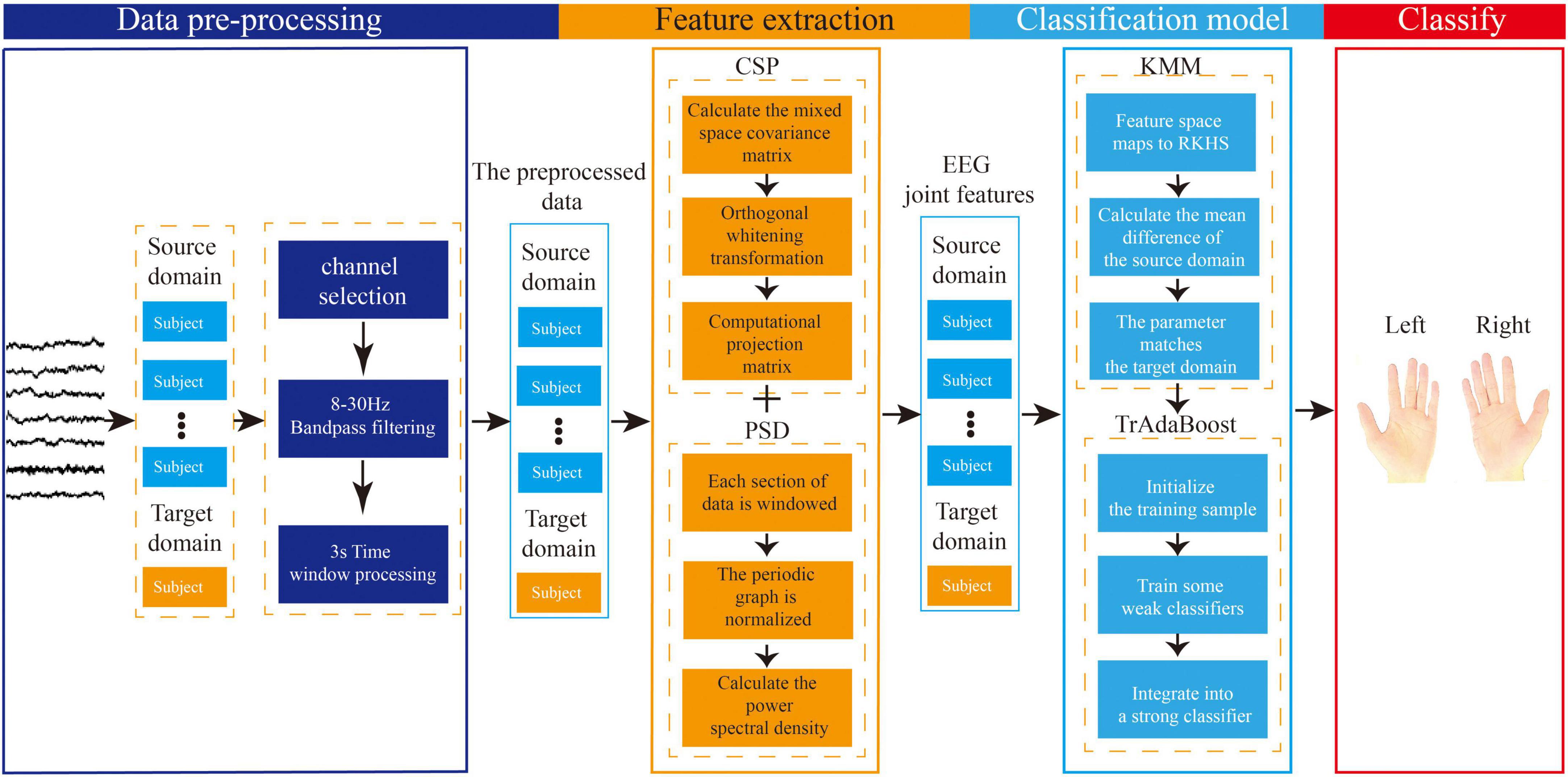
Figure 7. Flowchart of electroencephalography (EEG) joint feature classification algorithm based on instance transfer and ensemble learning.

(1) In the data preprocessing part, channel selection, band-pass filtering, and time window processing will be performed on the raw EEG data from the source and target domains.

(2) In the feature extraction part, the preprocessed data from the source and target domains will be used for feature extraction. The spatial features will be extracted based on the CSP algorithm, and the frequency features will be extracted based on the PSD algorithm using Welch’s method. Finally, the spatial and frequency features will be combined to form the joint EEG features.

(3) In the ensemble learning classification part, the sample weights of the joint features obtained from the source and target domains will be adjusted using the KMM algorithm to make the source and target domains as close as possible, and the sample weight matrix will be obtained. Then, this matrix will be used as the initialization weight matrix in the TrAdaBoost algorithm and used to initialize the training samples. Next, multiple weak classifiers will be trained using the initialized training data, and finally, a strong classifier will be obtained using a weighted voting strategy based on the weights of each weak classifier, achieving the goal of using ensemble learning for MI-EEG classification.

4. Experiment analysis

4.1. Result evaluation index

In this study, The Accuracy (ACC) was selected as an indicator to evaluate the performance of the classification model, and the calculation formula is as follows:

$Acc=\frac{TP+TN}{TP+TN+FP+FN}(17)$

Where, _TP and _TN represent the number of samples correctly classified as positive labels and negative labels, respectively. _FP and _FN are the number of samples misclassified as positive labels and negative labels, respectively.

4.2. Comparative experiment and results analysis

In this study, EEG data from nine subjects (A01, A02,…, A09) in the BCI Competition IV Dataset 2a, as well as EEG data from nine subjects (B01, B02,…, B09) in the BCI Competition IV Dataset 2b, will be selected as research data. During each experiment targeting each dataset, EEG data from eight subjects were selected as source domain data, and data from another subject was selected as target domain data. To validate the effectiveness of our proposed EEG joint feature classification algorithm based on instance transfer and ensemble learning (Ours), several comparative experiments will be designed, including CSP+SVM, PSD+SVM, CSP+PSD+SVM, CSP+PSD+KMM, and CSP+PSD+TrAdaBoost.

(1) CSP+SVM, PSD+SVM, and CSP+PSD+SVM were taken as a group of comparative experiments. The spatial domain features, frequency domain features, and EEG joint features were, respectively classified by SVM algorithm. The average classification accuracies for these three experiments are 66.8, 58.9, and 73.2% in Dataset 2a, and 64.7, 60.4, and 70.1% in Dataset 2b, respectively. The CSP+PSD+SVM achieved the best classification effect, indicating that the joint spatial and frequency domain features can improve the classification performance of MI-EEG. However, its classification accuracy is lower than Ours by about 18 and 13% in Dataset 2a and Dataset 2b, respectively, mainly due to the large individual differences in MI-EEG among different subjects, and the trained models of other subjects cannot be well-applied to the current subject. This also confirms that the K-T algorithm utilizing instance transfer method can effectively solve the problem of individual differences among different subjects.

(2) CSP+PSD+TrAdaBoost algorithm: The average classification accuracy obtained by using the TrAdaBoost algorithm to classify the joint features of EEG is only 81.3 and 76.2% in Dataset 2a and Dataset 2b, respectively, which is lower than the classification accuracy of Ours. The main reason is that the distribution of data in source domain and target domain is different, and the TrAdaBoost algorithm uses the same weight as the initial weight matrix during classification initialization, which leads to unreasonable sample weights. In this case, if KMM algorithm is used to adjust the sample weight matrix, the data can be distributed more reasonably.

(3) CSP+PSD+KMM algorithm: The average classification accuracy obtained by using the KMM algorithm to classify the joint features of EEG is only 84.3 and 76.4% in Dataset 2a and Dataset 2b, respectively, which is lower than the classification accuracy of Ours. The main reason is that KMM needs to estimate a kernel density ratio, and the error of this ratio estimate negatively affect the performance of domain adaptation. In this case, if the TrAdaBoost algorithm is used to reassign different weights to the source domain and target domain to reduce the influence of estimation errors in KMM algorithm, the performance of domain adaptation can be improved.

From Table 1, Figure 8, it can be seen that for the same classification method, using the EEG joint features as the feature vector can significantly improve the average classification accuracy by 6–14% and 5–10% in Dataset 2a and Dataset 2b, respectively, compared to using the feature vector from a single domain. It shows that EEG joint features can break through the limitations of single domain EEG features, provide more comprehensive and detailed EEG analysis, and improve the classification performance of MI-EEG.

TABLE 1

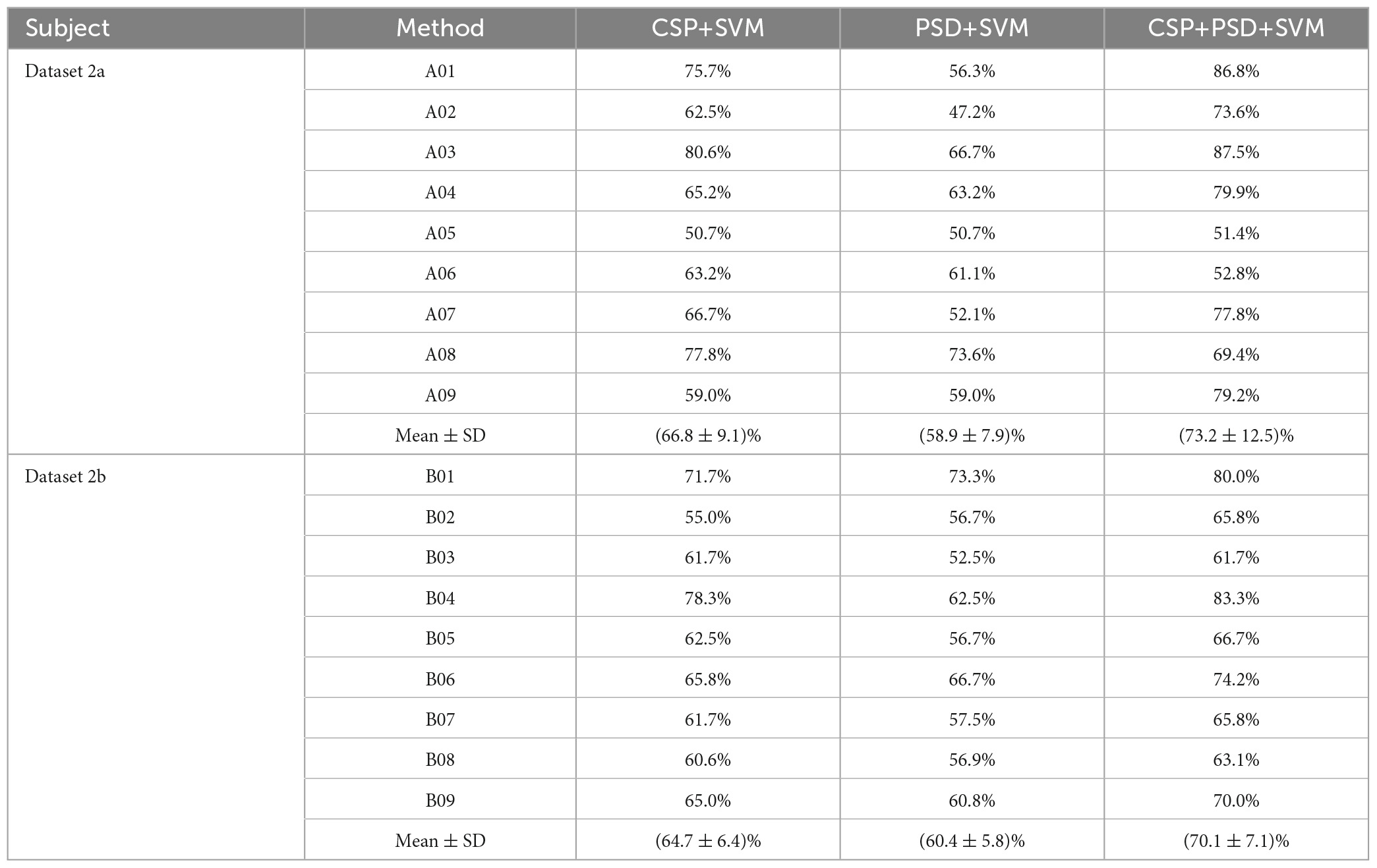
Table 1. Comparison of classification accuracy among the three methods for nine subjects in Dataset 2a and Dataset 2b in the first group of experiments.

FIGURE 8

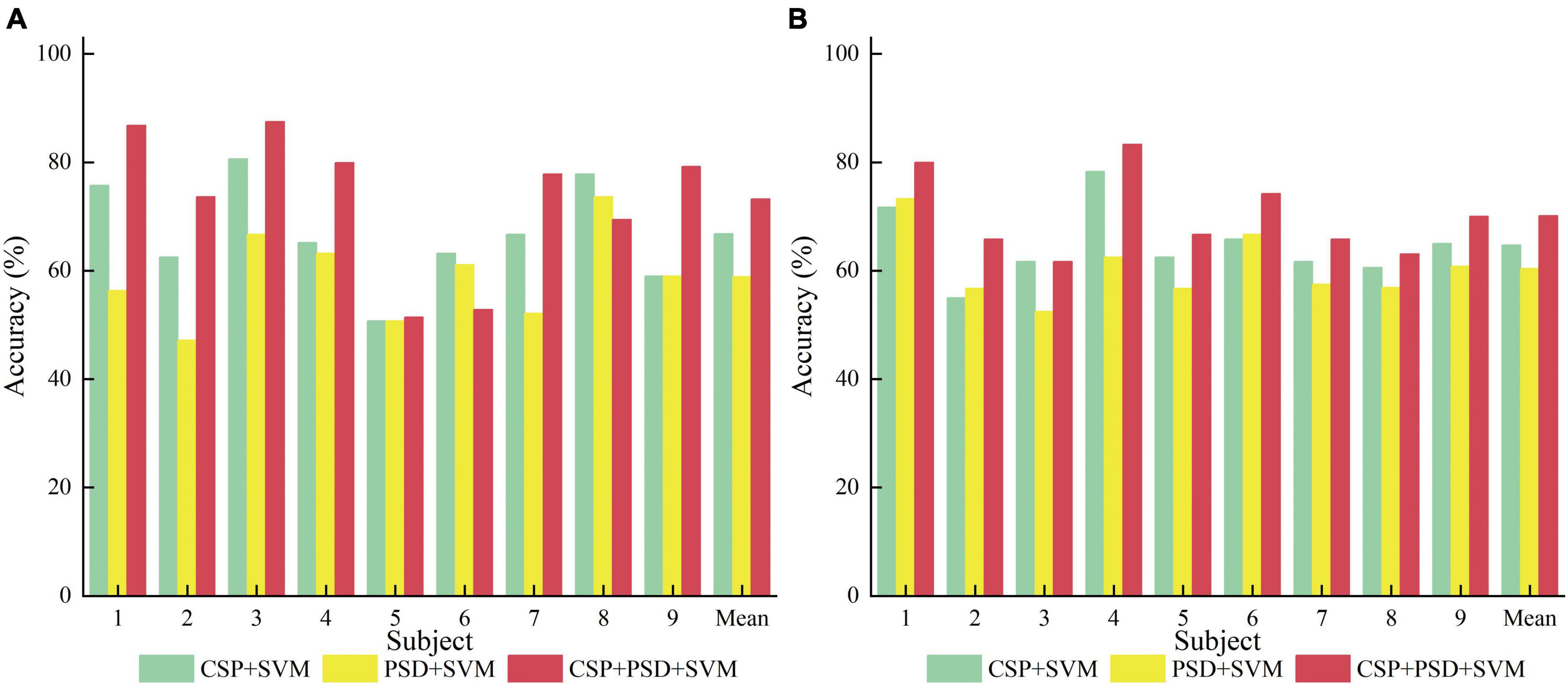
Figure 8. Comparison of classification accuracy among three methods for nine subjects in the first group of experiments. (A) Dataset 2a. (B) Dataset 2b.

According to Tables 2, 3, and Figure 9, when EEG joint features are used as feature vectors, the average classification accuracy obtained by Ours algorithm in Dataset 2a is 18.3, 10.2, and 7.2% higher than that obtained by SVM algorithm, TrAdaBoost algorithm and KMM algorithm, respectively. They were 13.6, 7.5, and 7.3% higher in Dataset 2b. It is explained that Ours, considering that TrAdaBoost algorithm can improve the performance of classifier and reduce the classification error rate through sample weighting. At the same time, it is also considered that the KMM algorithm can further improve the matching of sample distribution by distributing the importance weight of samples. Therefore, by using K-T ensemble learning, several weak classifiers can be integrated into strong classifiers through sample importance weight allocation and weighted classifiers, so as to eliminate individual differences among different subjects, so as to improve the generalization ability of classification model and improve the classification performance of MI-EEG.

TABLE 2

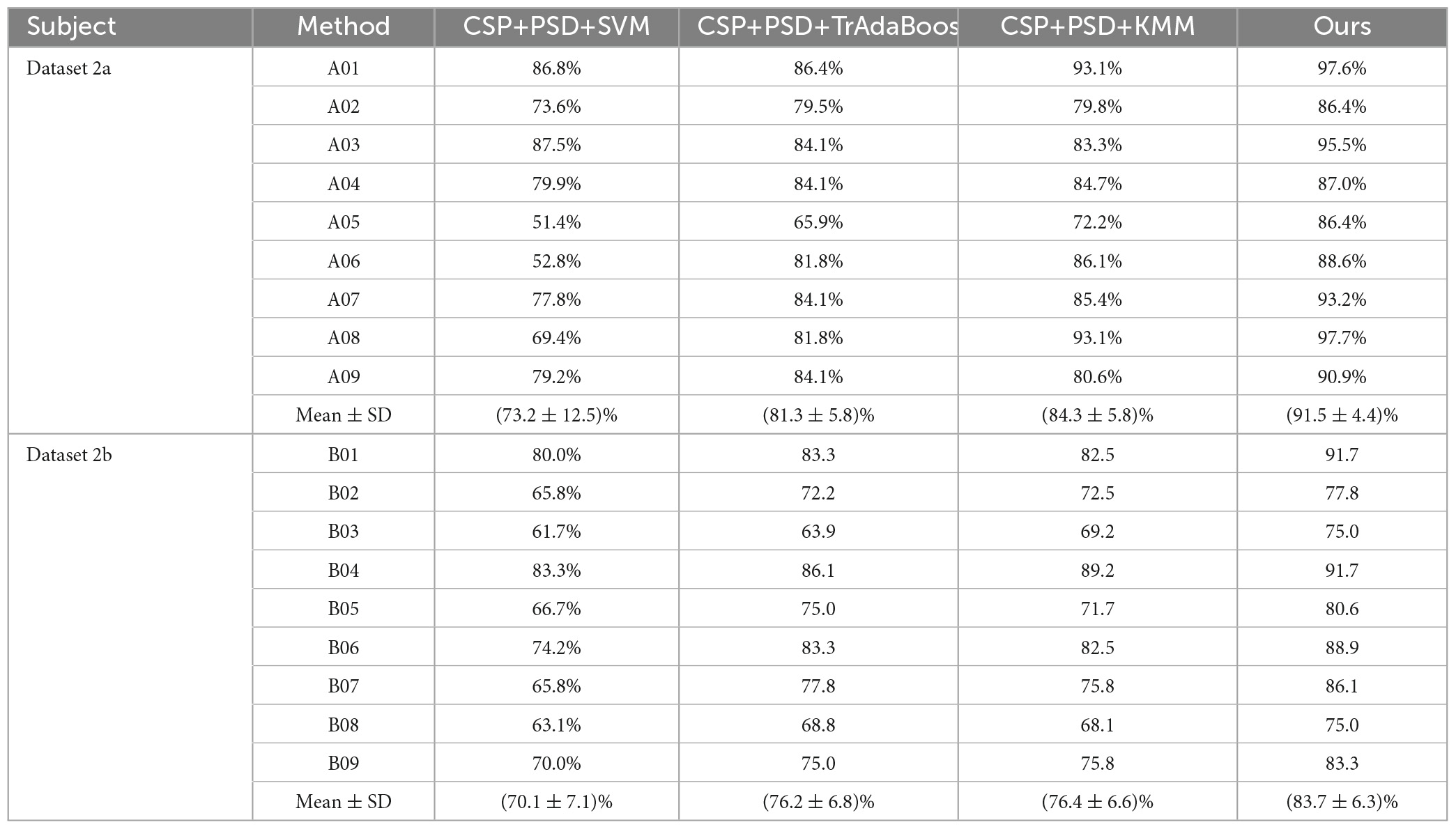
Table 2. Comparison of classification accuracy between the proposed method and the comparative experimental method in Dataset 2a and Dataset 2b.

TABLE 3

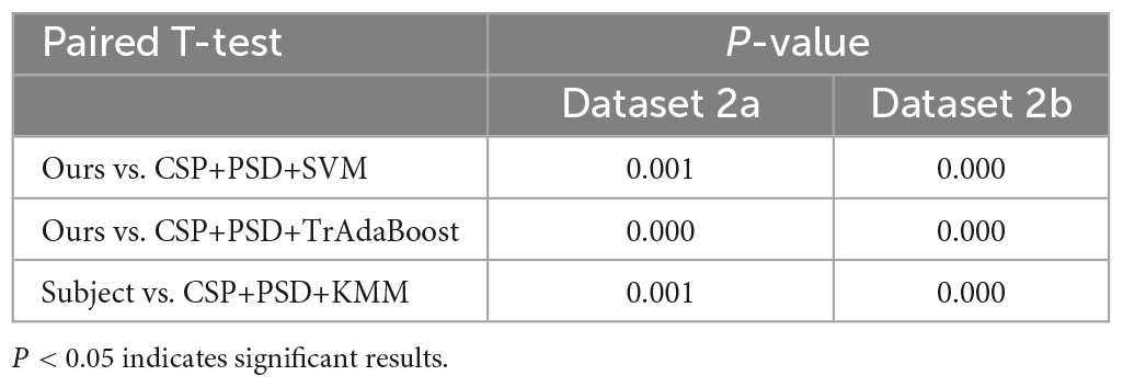
Table 3. T-test results of the proposed method and the comparative experimental method.

FIGURE 9

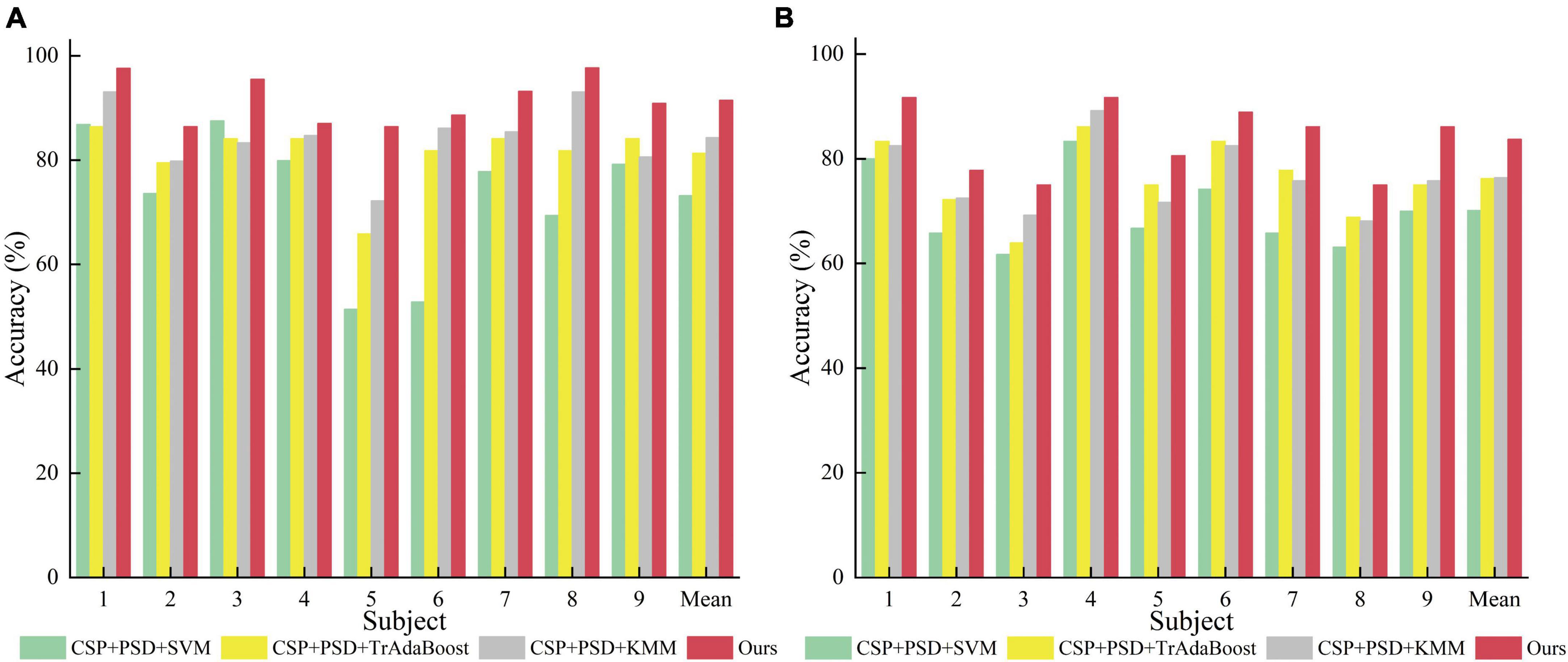
Figure 9. Comparison of classification accuracy between the proposed method and the comparative experimental method. (A) Dataset 2a. (B) Dataset 2b.

4.3. Comparison with state-of-the-art methods

In order to verify the superiority of the algorithm proposed in this paper, it is compared with algorithms proposed by other researchers in the same data set (BCI Competition IV Dataset 2a), and the experimental results are shown in Table 4 and Figure 10. As can be seen from the table, the accuracy of subjects five and six is very low in other literatures, but in Ours, it is significantly improved by more than 13%. In addition, compared with the methods of other researchers, the average classification accuracy of Ours was increased by more than 10%, indicating that Ours outperforms other algorithms in the classification performance of MI-EEG.

TABLE 4

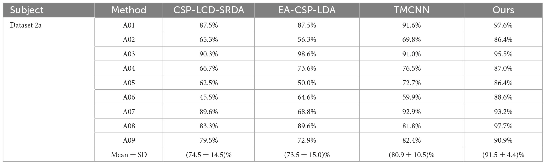
Table 4. Comparison of classification accuracy of the method presented in this paper and the methods proposed by other researchers on brain-computer interface (BCI) competition IV dataset 2a.

FIGURE 10

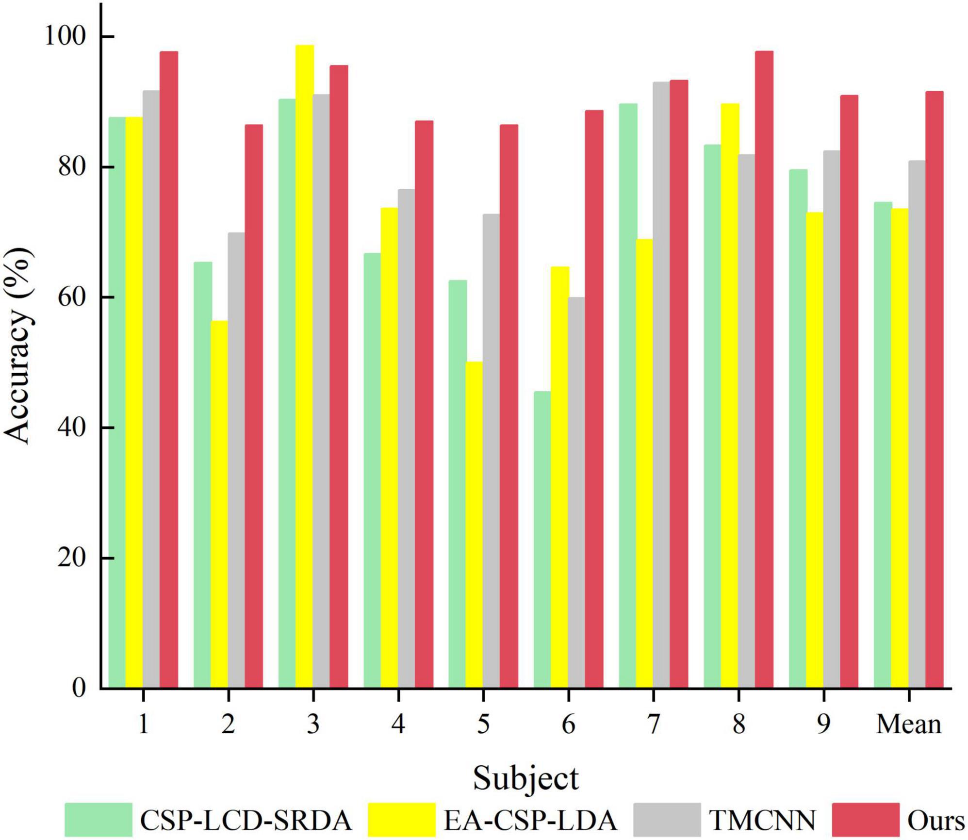
Figure 10. Comparison of classification accuracy between the proposed method and other methods.

5. Conclusion

During the process of motor imagery, there are asymmetric energy differences in the spatial brain area. Therefore, researchers usually use the CSP algorithm to extract distinctive spatial features from multi-channel EEG. In addition, since EEG are mainly rhythmic signals, ERD and ERS occur within specific frequency bands, and CSP algorithm directly performs spatial filtering on frequency domain signals, so frequency domain information is crucial for MI task classification and cannot be ignored. Therefore, in order to fully explore EEG and enrich EEG features and improve the recognition of MI signals, this paper proposes to use CSP and PSD to extract spatial and frequency domain features, respectively, and combine them to obtain EEG joint features, providing a more comprehensive and detailed analysis of EEG. In addition, the sample size of individual training for MI-EEG is small, and there are great individual differences among different subjects. This paper proposes a joint feature classification algorithm for EEG based on instance transfer and ensemble learning. After obtaining the EEG joint features, KMM and TrAdaboost are combined, and an ensemble learning strategy is used to integrate a classifier with strong generalization ability. The experimental results show that the algorithm has an average accuracy of 91.5 and 83.7% on Dataset 2a and Dataset 2b, respectively, which is significantly better than other algorithms and provides a new approach to solving the above problems. However, it may not be applicable to other EEG data such as P300 and emotion recognition data. Therefore, in future research, we can make the algorithm applicable to other EEG signal data by improving the alignment between the source domain and the target domain.

Data availability statement

The original contributions presented in this study are included in the article/supplementary material, further inquiries can be directed to the corresponding authors.

Author contributions

XW and XD designed the research. XW wrote the manuscript. RH and ML collected the data and supervised the study. XC, YL, and QH supervised and revised the manuscript. All authors contributed to the article and approved the submitted version.

Funding

This work was supported by the National Natural Science Foundation of China (Nos. 81960324 and 62176104), Natural Science Foundation of Guangxi Province (2021GXNSFAA075037), Innovation Project of Guangxi Graduate Education (No. YCSW2022436), and Medical Science and Technology Research Foundation of Guangdong Province (A2021138).

Conflict of interest

The authors declare that the research was conducted in the absence of any commercial or financial relationships that could be construed as a potential conflict of interest.

Publisher’s note

All claims expressed in this article are solely those of the authors and do not necessarily represent those of their affiliated organizations, or those of the publisher, the editors and the reviewers. Any product that may be evaluated in this article, or claim that may be made by its manufacturer, is not guaranteed or endorsed by the publisher.

References

Ai, Q., Chen, A., Chen, K., Liu, Q., Zhou, T., Xin, S., et al. (2019). Feature extraction of four-class motor imagery EEG signals based on functional brain network. J. Neural Eng. 16:026032. doi: 10.1088/1741-2552/ab0328

PubMed Abstract | CrossRef Full Text | Google Scholar

Amirhossein, A. S., Mahanta, M. S., and Konstantinos, N. P. (2016). Separable common spatio-spectral patterns for motor imagery BCI systems. IEEE Trans. Biomed. Eng. 63, 15–29. doi: 10.1109/TBME.2015.2487738

PubMed Abstract | CrossRef Full Text | Google Scholar

Bastien, O., Kyuhwa, L., Ricardo, C., and Millan, J. (2020). User adaptation to closed-loop decoding of motor imagery termination. IEEE Trans. Biomed. Eng. 68, 3–10. doi: 10.1109/TBME.2020.3001981

PubMed Abstract | CrossRef Full Text | Google Scholar

Bin, N., Saidatul, A., Chong, Y., and Ibrahim, Z. (2019). PSD-based features extraction for EEG signal during typing task. Mater. Sci. Eng. 557:012032. doi: 10.1088/1757-899x/557/1/012032

CrossRef Full Text | Google Scholar

Cao, J., Hu, D., Wang, Y., Wang, J., and Lei, B. (2021). Epileptic classification with deep-transfer-learning-based feature fusion algorithm. IEEE Trans. Cogn. Dev. Syst. 14, 684–695. doi: 10.1109/TCDS.2021.3064228

CrossRef Full Text | Google Scholar

Chen, L. F., Li, M., Su, W., Wu, M., Kaoru, H., Pedrycz, W., et al. (2021). Adaptive feature selection-based AdaBoost-KNN with direct optimization for dynamic emotion recognition in human-robot interaction. IEEE Trans. Emerg. Top. Comput. Intell. 5, 205–213. doi: 10.1109/TETCI.2019.2909930

CrossRef Full Text | Google Scholar

Chen, l, Gong, A., Ding, P., and Fu, Y. (2022). EEG signal decoding of motor imagination based on euclidean space–weighted logistic regression transfer learning. J. Nanjing Univ. 58, 264–274. doi: 10.13232/j.cnki.jnju.2022.02.010

CrossRef Full Text | Google Scholar

Dai, W., Qiang, Y., Xue, G., and Yong, Y. (2007). “Boosting for transfer learning,” in Proceedings of the 24th International Conference on Machine Learning, (Corvalis, OR), 20–24. doi: 10.1145/1273496.1273521

CrossRef Full Text | Google Scholar

Feng, B., Chen, X., Chen, Y., Yu, T., Duan, X., Liu, K., et al. (2023). Identifying solitary granulomatous nodules from solid lung adenocarcinoma: Exploring robust image features with cross-domain transfer learning. Cancers 15:892. doi: 10.3390/cancers15030892

PubMed Abstract | CrossRef Full Text | Google Scholar

Feng, B., Huang, L., Liu, Y., Chen, Y., Zhou, H., Yu, T., et al. (2022). A transfer learning radiomics nomogram for preoperative prediction of borrmann type IV gastric cancer from primary gastric lymphoma. Front. Oncol. 11:802205. doi: 10.3389/fonc.2021.802205

PubMed Abstract | CrossRef Full Text | Google Scholar

Gertton, A., Borgwardt, K. M., Rasch, M., Schlkopf, B., and Smola, A. (2012). A kernel two-sample test. J. Mach. Learn. Res. 13, 723–773. doi: 10.1142/S0219622012400135

CrossRef Full Text | Google Scholar

He, H., and Wu, D. (2019). Transfer Learning for brain-computer interfaces: A euclidean space data alignment approach. IEEE Trans. Biomed. Eng. 67, 399–410.

Google Scholar

Holmes, P., and Calmels, C. (2008). A neuroscientific review of imagery and observation use in sport. J. Motor Behav. 40, 433–445. doi: 10.3200/JMBR.40.5.433-445

PubMed Abstract | CrossRef Full Text | Google Scholar

Li, M., Yang, L., and Yang, J. (2011). A online self-learning approach to EEG classification. Comput. Meas. Control 19, 2763–2765. doi: 10.16526/j.cnki.11-4762/tp.2011.11.042

CrossRef Full Text | Google Scholar

Manali, S., Udit, S., and Madhur, D. (2020). Wavelet based waveform distortion measures for assessment of denoised EEG quality with reference to noise-free EEG signal. IEEE Signal Process. Lett. 27, 1260–1264. doi: 10.1109/LSP.2020.3006417

CrossRef Full Text | Google Scholar

Miltona, J., Small, S. L., and Solodkin, A. (2008). Imaging motor imagery: Methodological issues related to expertise. Methods 45, 336–341. doi: 10.1016/j.ymeth.2008.05.002

PubMed Abstract | CrossRef Full Text | Google Scholar

Qiu, L., Zhong, Y., He, Z., and Pan, J. (2022). Improved classification performance of EEG-fNIRS multimodal brain-computer interface based on multi-domain features and multi-level progressive learning. Front. Hum. Neurosci. 16:973959. doi: 10.3389/fnhum.2022.973959

PubMed Abstract | CrossRef Full Text | Google Scholar

Ramoser, H., Muller-Gerking, J., and Pfurtscheller, G. (2000). Optimal spatial filtering of single trial EEG during imagined hand movement. IEEE Trans. Rehabil. Eng. 8, 441–446. doi: 10.1109/86.895946

PubMed Abstract | CrossRef Full Text | Google Scholar

Tangermann, M., Müller, K., Aertsen, A., Birbaumer, N., Braun, C., Brunner, C., et al. (2012). Review of the BCI Competition IV. Front. Neurosci. 13:55. doi: 10.3389/fnins.2012.00055

PubMed Abstract | CrossRef Full Text | Google Scholar

Wolpaw, J. R., Birbaumer, N., McFarland, D. J., Pfurtscheller, G., and Vaughan, T. M. (2002). Brain-computer interfaces for communication and control. Clin. Neurophysiol. 113, 767–791. doi: 10.1016/s1388-2457(02)00057-3

PubMed Abstract | CrossRef Full Text | Google Scholar

Xing, D., Dai, W., Xue, G., and Yu, Y. (2007). Bridged refinement for transfer learning. Eur. Conf. Princ. Pract. Knowl. Discov. Databases 4702, 324–335. doi: 10.1007/978-3-540-74976-9_31

CrossRef Full Text | Google Scholar

Xu, B. G., He, X. H., Wei, Z. W., Song, A. G., and Zhao, G. P. (2018). Research on continuous control system for Robot based on motor imagery EEG. Chin. J. Sci. Instr. 39, 10–19. doi: 10.19650/j.cnki.cjsi.J1803518

CrossRef Full Text | Google Scholar

Zhang, X., Hou, W., Wu, X., Feng, S., and Chen, L. (2021). A novel online action observation-based brain-computer interface that enhances event-related desynchronization. IEEE Trans. Neural Syst. Rehabil. Eng. 29, 2605–2614. doi: 10.1109/TNSRE.2021.3133853

PubMed Abstract | CrossRef Full Text | Google Scholar

Zhou, Q., and Tian, P. (2021). EEG identification algorithm of motor imagination based on multi-level fusion of transfer learning. Chin. J. Sci. Instr. 35, 174–181. doi: 10.13382/j.jemi.B2103864

CrossRef Full Text | Google Scholar