 Sourav Halder1Ethan M. Johnson2Jun Yamasaki3Peter J. Kahrilas4Michael Markl3John E. Pandolfino4Neelesh A. Patankar1,3*
- 1Theoretical and Applied Mechanics Program, McCormick School of Engineering, Northwestern University, Evanston, IL, United States
- 2Department of Radiology, Feinberg School of Medicine, Northwestern University, Chicago, IL, United States
- 3Department of Mechanical Engineering, McCormick School of Engineering, Northwestern University, Evanston, IL, United States
- 4Department of Medicine, Feinberg School of Medicine, Division of Gastroenterology and Hepatology, Northwestern University, Chicago, IL, United States
Dynamic magnetic resonance imaging (MRI) is a popular medical imaging technique that generates image sequences of the flow of a contrast material inside tissues and organs. However, its application to imaging bolus movement through the esophagus has only been demonstrated in few feasibility studies and is relatively unexplored. In this work, we present a computational framework called mechanics-informed MRI (MRI-MECH) that enhances that capability, thereby increasing the applicability of dynamic MRI for diagnosing esophageal disorders. Pineapple juice was used as the swallowed contrast material for the dynamic MRI, and the MRI image sequence was used as input to the MRI-MECH. The MRI-MECH modeled the esophagus as a flexible one-dimensional tube, and the elastic tube walls followed a linear tube law. Flow through the esophagus was governed by one-dimensional mass and momentum conservation equations. These equations were solved using a physics-informed neural network. The physics-informed neural network minimized the difference between the measurements from the MRI and model predictions and ensured that the physics of the fluid flow problem was always followed. MRI-MECH calculated the fluid velocity and pressure during esophageal transit and estimated the mechanical health of the esophagus by calculating wall stiffness and active relaxation. Additionally, MRI-MECH predicted missing information about the lower esophageal sphincter during the emptying process, demonstrating its applicability to scenarios with missing data or poor image resolution. In addition to potentially improving clinical decisions based on quantitative estimates of the mechanical health of the esophagus, MRI-MECH can also be adapted for application to other medical imaging modalities to enhance their functionality.
1 Introduction
The esophagus plays a crucial role in the functioning of the gastrointestinal tract, and esophageal disorders are associated with reduced quality of life. There is a high worldwide prevalence of esophageal disorders, as exemplified by studies (El-Serag et al., 2014; Yamasaki et al., 2018) reporting that gastroesophageal reflux disease (GERD) has a prevalence of
Previous mechanics-based studies on the esophagus have been conducted both experimentally and computationally. Experimental studies (Fan et al., 2004; Yang et al., 2006; Natali et al., 2009; Stavropoulou et al., 2009; Sokolis, 2013) focused on the mechanical properties of the esophageal walls in vitro. In silico modeling of the esophagus has been performed both in the context of pure fluid mechanics (Brasseur, 1987; Li and Brasseur, 1993; Li et al., 1994; Ghosh et al., 2005; Acharya et al., 2021a) to understand the nature of bolus transport and in fully resolved fluid-structure interaction models to understand how the esophageal muscle architecture influences esophageal transport and the stresses developed in the esophageal walls during bolus transport (Kou et al., 2015; Kou et al., 2017; Halder et al., 2022a). A systematic review of the various constitutive models of the esophagus and the other organs of the gastrointestinal tract was conducted by Patel et al. (2022). In silico mechanics-based analyses (Acharya et al., 2021b; Halder et al., 2021; Halder et al., 2022b) have also been performed on data obtained from various diagnostic devices to identify mechanics-based physiomarkers. Acharya et al. (2021b) used a mechanics-based approach to calculate the work carried out by the esophagus in opening the esophagogastric junction (EGJ) and the necessary work required to open the EGJ using data obtained from FLIP. Halder et al. (2021) introduced a framework called FluoroMech applied to fluoroscopy images to estimate the mechanical health of the esophagus through quantitative estimates of esophageal wall stiffness and active relaxation. FluoroMech enhances the capability of fluoroscopy by adding quantitative predictions to fluoroscopy data, which are inherently qualitative in nature. In this work, we present a framework called MRI-MECH, which uses dynamic MRI as input to estimate esophageal health through mechanics-based metrics for active relaxation and wall stiffness.
Both FluoroMech and MRI-MECH utilize the input of esophageal cross-sectional area, which varies as a function of time and length along the esophagus. However, there are some key differences in their approach that can be classified into two categories. The first category pertains to the differences between fluoroscopy and dynamic MRI. Fluoroscopy is an older and simpler approach wherein X-ray imaging is used to visualize a swallowed bolus passing through the esophagus, resulting in a video with high temporal resolution but only a two-dimensional projection of the bolus. Hence, the three-dimensional geometry of the bolus is unknown. Fluoroscopy is a well-established clinical test. Dynamic MR imaging, on the other hand, is a relatively complicated and evolving technology. MRI has been used to detect esophageal cancers (Petrillo et al., 1990; Riddell et al., 2006), but dynamic MRI has been used only in limited feasibility studies (Panebianco et al., 2006; Kulinna-Cosentini et al., 2007; Marciani, 2011). Most of these studies visualize esophageal wall movement through 2D imaging sequences using orally administered Gd contrast. In their current state, dynamic MRI images have a significantly lower temporal resolution but a very detailed three-dimensional representation of the bolus. However, dynamic MR imaging is currently not a standard practice for evaluating esophageal disorders, offering a vast potential for improvement. The second category of differences between FluoroMech and MRI-MECH lies in the implementations of the frameworks. FluoroMech uses the finite volume method to predict esophageal wall stiffness and active relaxation with the variation of the cross-sectional area as input. It is computationally fast (less than a minute) and requires very limited computational resources, but it requires a complete dataset of the variation of the cross-sectional area. Assumptions are required regarding the 3D shape of the bolus based on the volume of fluid swallowed, and since model predictions are sensitive to cross-sectional area variation, inaccuracies in measurements reflect on the predictions as well. MRI-MECH, on the other hand, uses a physics-informed neural network (PINN) (Raissi et al., 2019) to make predictions and is computationally demanding (takes approximately 1 hour to run), requiring better hardware, especially the GPU, to train the PINN. However, MRI-MECH is not sensitive to missing or imperfect measurements. Additionally, it does not require assumptions regarding the esophageal lumen cross-sectional shape because MRI provides three-dimensional geometry of the esophageal lumen. In the following sections, we describe the MRI-MECH framework in detail, along with its application to a dynamic MRI sequence.
2 Materials and methods
2.1 Accelerated dynamic MRI
Imaging was performed at 1.5 T (Aera, Siemens, Germany) using a 3D MR angiography sequence (TWIST, Siemens, Germany) designed for contrast-enhanced cardiac imaging applications, which was adapted to be used for esophageal imaging using pineapple juice as an oral contrast agent. Sequence parameters included
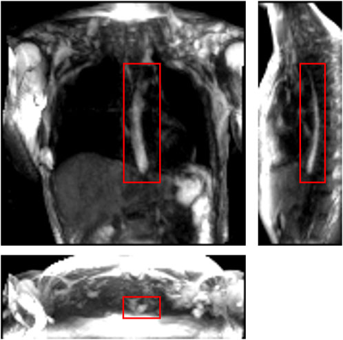
FIGURE 1. One instance of a dynamic MRI of a normal subject as seen in three perpendicular planes. The planes (from left to right to bottom) are coronal, sagittal, and axial, respectively. The bolus can be seen as the bright region inside the red boxes. Concentrated pineapple juice was swallowed as a contrast agent.
2.2 Extraction of bolus geometry
In this study, we used data from a single healthy volunteer to demonstrate this framework. The MRI output consisted of a cuboid wherein voxels in a Cartesian coordinate system had different magnitudes of intensity. The temporal resolution of the dynamic MRI (1.17 s) determined the number of images with the bolus seen within the esophagus: seven time instants in this study. The typical length of an adult esophagus is 18–25 cm (Oezcelik and DeMeester, 2011). The average velocity of normal peristalsis is approximately 3.3 cm/s (Hollis and Castell, 1975). Thus, an average swallow sequence usually takes 5–8 s. Therefore, temporal resolutions similar to what we used in our analysis typically result in 5–8 images. Although this temporal resolution is not comparable to fluoroscopy, the detailed three-dimensional geometry of the bolus in MRI leads to better prediction of velocity and intrabolus pressure, resulting in better prediction of esophageal wall properties. The bolus was manually segmented for the seven time instants, a few of which are shown in Figure 2. The segmentation assigned a value of 1 and 0 to each voxel that lay inside and outside the bolus, respectively. The image segmentation was performed using the open-source software ITK-SNAP (Yushkevich et al., 2006). With improved MR imaging and better temporal resolution, manual image segmentation might not be feasible, and more sophisticated automated segmentation techniques might be necessary. We have described in Supplementary Material S1 a deep learning-based automated segmentation approach called 3D-U-Net (Abdulkadir et al., 2016), which was fine-tuned for this application.
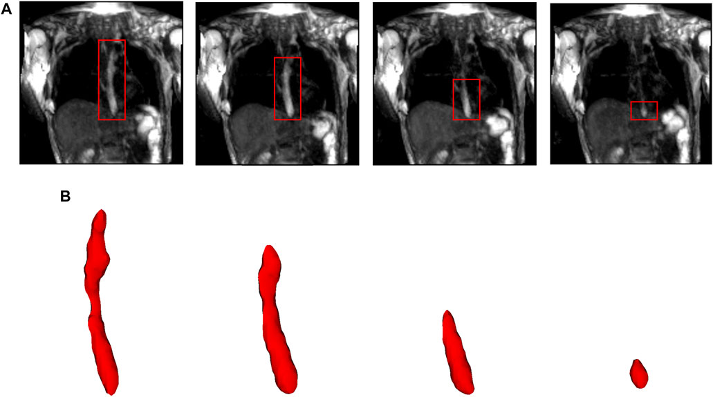
FIGURE 2. Segmentation of MR images. (A) The bolus is shown in the coronal plane at four time instants (progressing from left to right). The bolus is seen as the bright region inside the red boxes. The bolus volume decreased with time as it was emptied into the stomach. (B) The corresponding 3D segmented bolus shapes for the four time instants. The bolus size has been magnified for visualization.
MRI-MECH modeled the esophagus as a one-dimensional flexible tube. For such a one-dimensional analysis, the variation in cross-sectional areas at different points along the length of the esophagus and at different time instants had to be extracted from the three-dimensional bolus obtained from segmentation. This was performed in two steps. The first step was to generate a center line along the length of the esophagus. The bolus shapes observed at different time instants were superimposed, and then, cross-sections of the superimposed shape at different horizontal planes from the proximal to the distal end of the superimposed shape were generated. The centroids of these cross-sections were connected to form the center line. The length of the center line, in this case, was 9.65 cm. The second step, after extracting the center line, was to generate planes perpendicular to the center line, as shown in Figure 3. The segmented voxels marked 1, which lay near these perpendicular planes, were projected onto these planes. These projected points were connected using Delaunay triangulation, as shown in Figure 3. The cross-sectional area at each point along the center line was then calculated as the sum of the triangles in the Delaunay triangulated geometries.
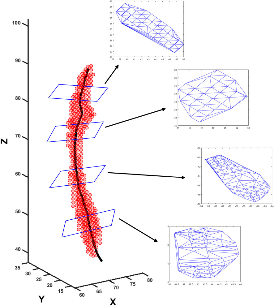
FIGURE 3. Extraction of cross-sectional areas from dynamic MR images. The segmented bolus geometry at one time instant is shown by the red points in the scatter plot. The generated center line is shown by the black curve inside. A few planes are shown that are perpendicular to the center line and on which the cross-sectional areas were calculated. The points on the planes were meshed using Delaunay triangulation, and the triangulated shapes approximate the cross-sectional areas at those planes.
2.3 MRI-MECH formulation
2.3.1 Governing equations
Transport through the esophagus was modeled as a one-dimensional fluid flow through a flexible tube. The mass and momentum conservation equations in one dimension (Barnard et al., 1966; Kamm and Shapiro, 1979; Ottesen, 2003; Manopoulos et al., 2006) are as follows:
where
It has been observed experimentally that the fluid pressure developed inside the esophagus is linearly proportional to the cross-sectional area of the esophageal lumen (Orvar et al., 1993; Kwiatek et al., 2011) in the absence of any neuromuscular activation. Using this information, a pressure tube law can be constructed as follows:
where
Due to the low resolution of the dynamic MRI, it was necessary to interpolate the MRI data to smaller temporal and spatial scales. The measured volume
where
The values of
where
where
2.3.2 Initial and boundary conditions
The boundary conditions of this problem were specified to capture the physiological conditions of normal esophageal transport. The upper esophageal sphincter (UES) at the proximal end of the esophagus opens to allow the bolus into the esophagus, closes once the fluid has passed through it, and remains closed thereafter. Hence, we specified zero velocity at
2.3.3 Cross-sectional area of the lower esophageal sphincter
The low spatial resolution of the dynamic MRI poses a problem in accurately identifying the lower esophageal sphincter (LES) cross-section. This is because the LES opening is narrower than the esophageal body and does not distend very much because of the greater wall stiffness at the EGJ. Although this could be improved by focusing the MRI only on the LES, the state of the esophagus proximal to the LES cannot be estimated in such a scenario. The LES can be identified in only 1 or 2 time instants when the LES has significantly distended due to bolus flow through it. Figure 4 shows the LES at one such time instant. The LES cross-sectional area measured at this time instant can act as a valuable reference to identify the bolus behavior proximal to the LES.
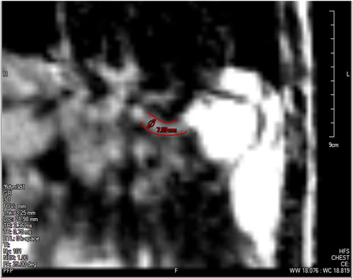
FIGURE 4. The lower esophageal sphincter identified at a single time instant outlined in red with a diameter of approximately 7.89 mm and a length of approximately 2.78 cm. The stomach can be seen to the right of the LES with the accumulated pineapple juice shown in bright white. The esophageal body cannot be seen in this slice because this plane does not intersect the esophagus.
As specified in the previous section, since pressure is specified as a Dirichlet boundary condition at the distal end of the esophagus, the intrabolus pressure prediction depends on the accurate measurement of the LES cross-sectional area. Figure 5 shows the intrabolus pressure calculated using the numerical approach described in the study by Halder et al. (2021) with different LES cross-sectional areas. The pressure shown is non-dimensional, and the pressure at the distal end was specified as zero as a reference in this case. The total length of the esophagus considered here is the sum of the center line length (9.65 cm) and the LES length (2.78 cm). Thus, the proximal and distal locations of the bolus were 9.65 cm and 12.43 cm, respectively. In non-dimensional form, the proximal and distal locations were
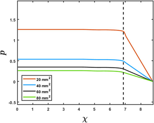
FIGURE 5. Effect of the LES cross-sectional area on the prediction of intrabolus pressure. The proximal end of the LES is marked by the vertical dashed line. The inserted legend shows LES cross-sectional areas used for this simulation. Eqs 7 and 8 were solved using the method described in FluoroMech (Halder et al., 2021) to calculate the intrabolus pressure. The input for the model was the variation of
2.3.4 Physics-informed neural network
The problem of missing data for the LES cross-sectional area (and consequently obtaining accurate intrabolus pressure values) was solved using a physics-informed neural network (Raissi et al., 2019). The problem description is schematically shown in Figure 6. The final interpolated volume
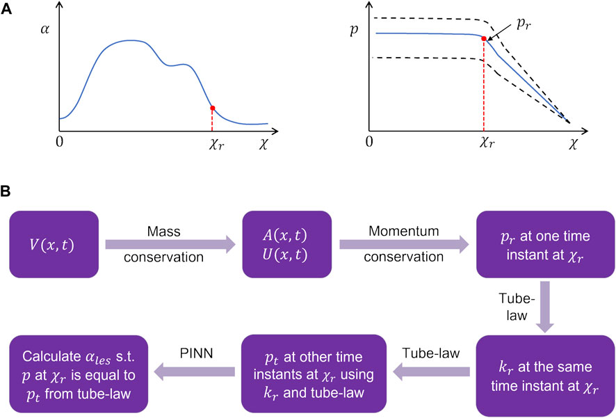
FIGURE 6. Problem definition for the physics-informed neural network framework. (A) Schematic for the variation in the cross-sectional area and pressure at the time instant when the LES cross-section was known. The dashed lines in the pressure variation show what intrabolus pressure would be at other time instants assuming constant LES cross-sectional area. (B) Workflow for the prediction of the LES cross-sectional area at other time instants.
It should be noted that there is no
The LES cross-sectional area (
where
2.3.4.1 Network architecture
The schematic in Figure 7 shows the architecture of the PINN. It takes
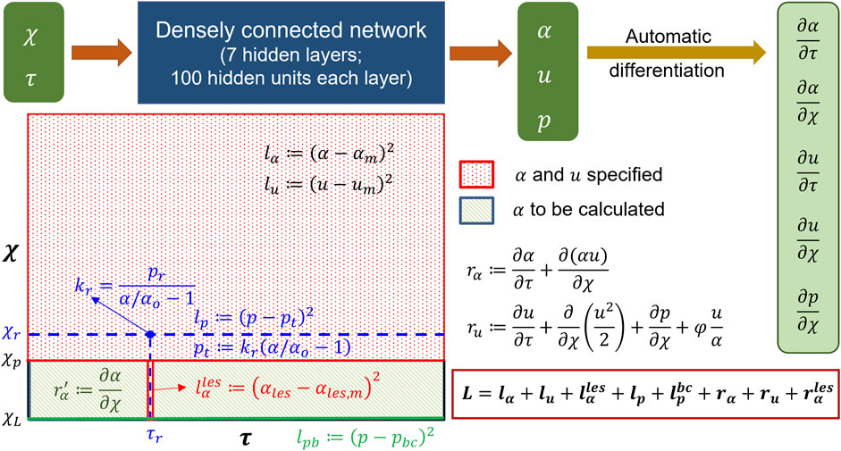
FIGURE 7. Details of the physics-informed neural network. The input and output of the PINN along with the details of the hidden layers are shown at the top. Automatic differentiation was used to calculate the derivative terms for the residuals. The schematic of the domain is shown in the following. The schematic describes where the different losses were specified.
2.3.4.2 Losses
The losses for the PINN consisted of a combination of measurement losses and residuals of the mass and momentum conservation equations. Minimizing the measurement losses ensures that the solutions are consistent with the measurements, and minimizing the residuals ensures that the governing physics behind the problem is followed. Figure 7 shows the locations and time instants at which the different measurement losses and residuals were calculated. As already mentioned in the workflow,
where the quantities with the subscript
where
where the point
where
where
where
To train the network, the inputs
where
2.3.4.3 Training
The network was trained using TensorFlow (MaA et al., 2016) for 100000 epochs. We used an Adam (DPaB, 2014) optimizer to minimize the losses. A piecewise constant decayed learning rate was used to minimize the losses efficiently. The learning rate was 0.001 for the first 10000 epochs, 0.0001 for the next 20000 epochs, and 0.00003 for the last 70000 epochs. The final values for
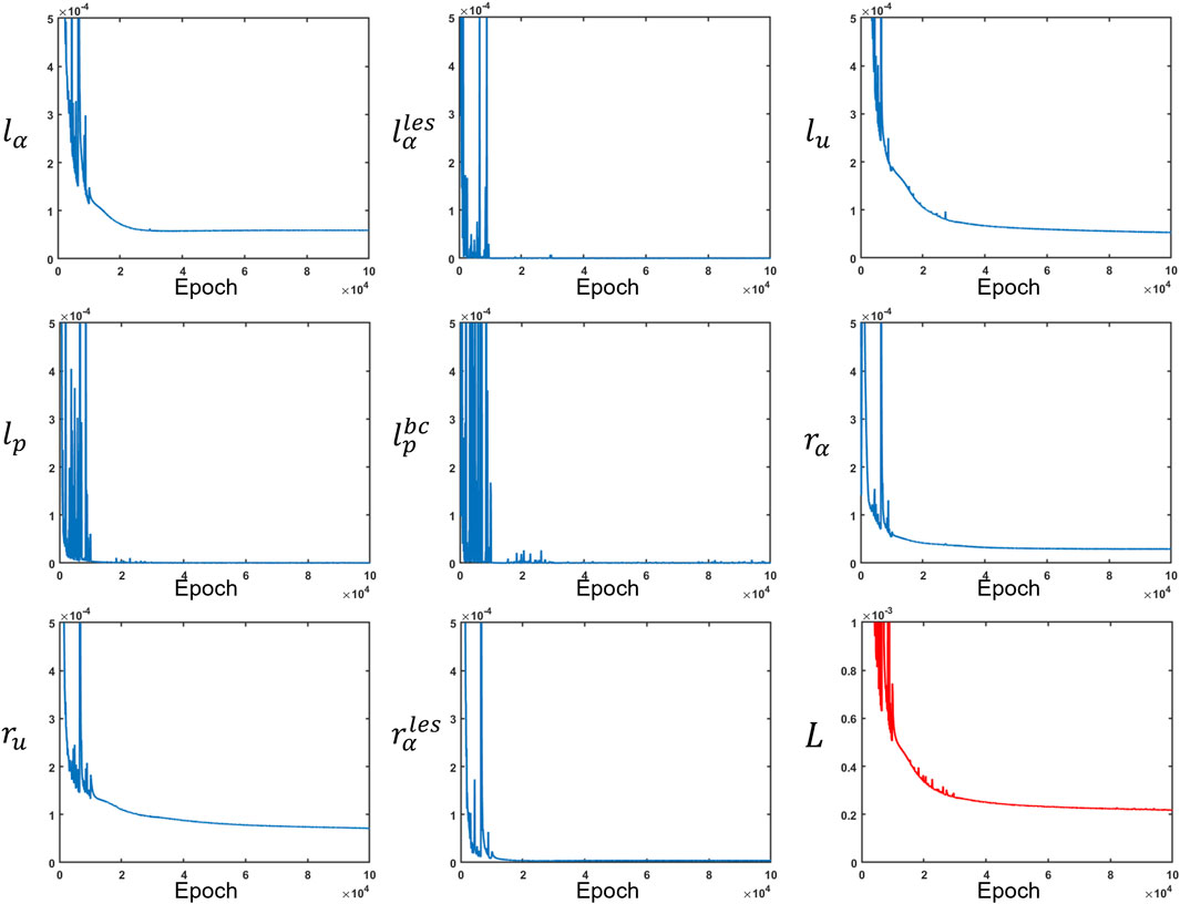
FIGURE 8. Measurement losses and residuals along with the total loss. All loss functions were minimized at different rates. The total loss is depicted in red, while the other losses are in blue.
2.3.4.4 Verification using the method of manufactured solutions
The PINN predictions of
where
Finally, we assumed an expression for pressure according to Eq 9 with
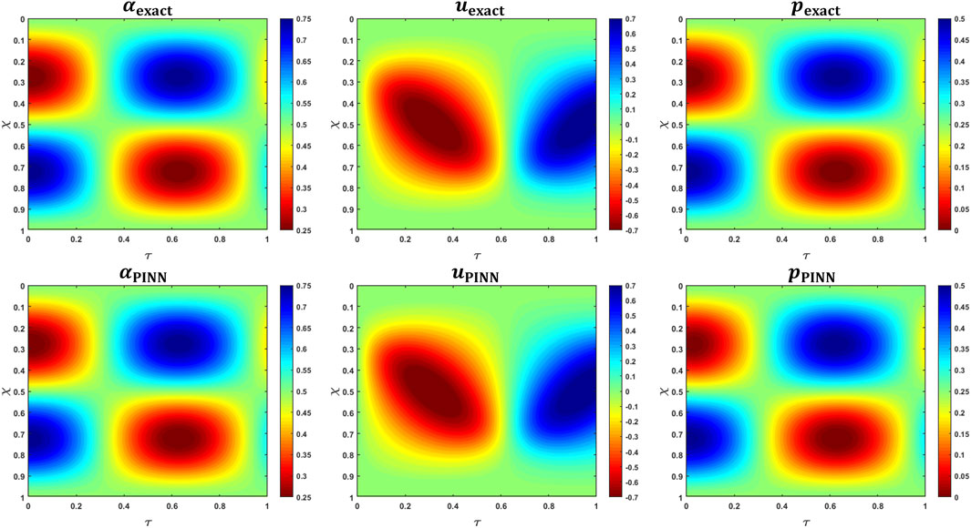
FIGURE 9. MMS verification of PINN predictions. The top row shows the variations in the analytical expressions for
2.3.5 Esophageal wall stiffness and active relaxation
The esophageal wall stiffness and active relaxation were calculated as described in the study by Halder et al. (2021). A few manipulations of Eq 3 yield the following:
The active relaxation parameter
where
where
3 Results and discussion
The PINN predicts the non-dimensional cross-sectional area, fluid velocity, and fluid pressure by minimizing a set of measurement losses and ensuring that the physics of the fluid flow problem is followed throughout. The variation in the predicted cross-sectional area (in its dimensional form) as a function of

FIGURE 10. Variation in the cross-sectional area as predicted by the PINN. (A) Variation in A as a function of x and t. The dashed white line indicates the proximal end of the LES. The cross-sectional area above the dashed line was known from MRI, and its prediction by the PINN was ensured by minimizing Eq 13. There is no variation in A along x within the LES due to the constraint described in Eq 12, (B) Variation in the LES cross-sectional area as a function of time. It had the greatest magnitude near the instant such that the LES was visible in the MRI image.
The cross-sectional areas proximal to the bolus cannot be visualized in MRI because the fluid contrast medium was completely displaced by the peristaltic contraction, and dynamic MR imaging cannot distinguish the esophagus from surrounding tissues. Hence, we assigned the inactive cross-sectional area
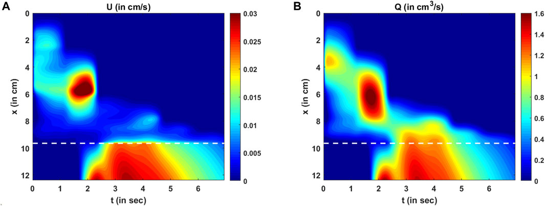
FIGURE 11. Variations in velocity and flow rate. (A) Variation in U as predicted by the PINN. There are two high-velocity zones: one at x = 6 cm, t = 2 s and the other at the LES for t > 2 s. These high-velocity zones match the regions of low cross-sectional areas. (B) Variation in the mean flow rate calculated as Q = AU. The high flow rate matches the high-velocity zones, but there is a smoother transition of Q at the proximal end of the LES compared to U.
The variation in the LES cross-sectional area is shown more clearly in Figure 10B. The prediction of
The variations in bolus fluid velocity and flow rate are shown in Figures 11A, B, respectively. There are two major high-velocity zones. The first high-velocity zone is near
The variation in fluid pressure is shown in Figure 12. The pressure gradients along
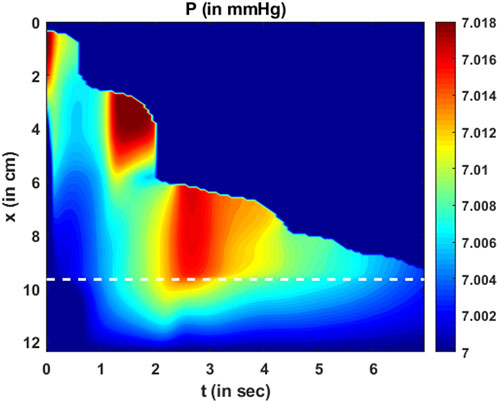
FIGURE 12. Variation in pressure as a function of
The total intrabolus pressure, as shown in Figure 12, is within the normal range according to CCv4.0, leading us to conclude that our specifications for intragastric pressure and thoracic pressure were valid. The prediction of
Esophageal wall stiffness (along with the effect of active relaxation) was estimated by the parameter
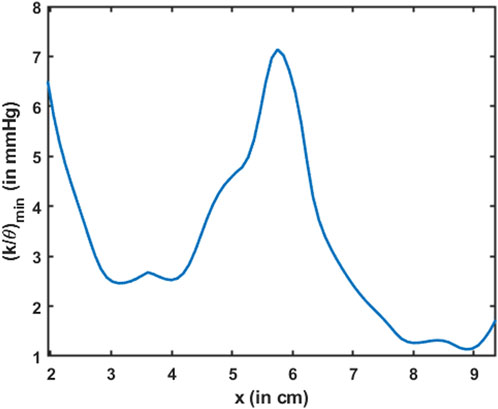
FIGURE 13. Variation in the minimum esophageal wall stiffness along the length of the esophagus. This measure of stiffness accounts for active relaxation and captures the wall characteristics when the esophagus was distended. The stiffness is shown only for the esophageal body proximal to the LES.
The parameter
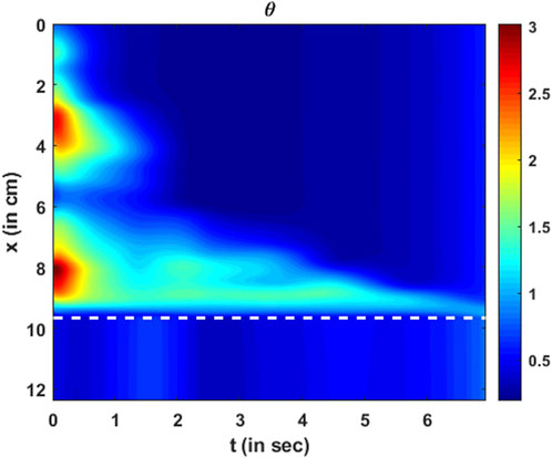
FIGURE 14. Variation in active relaxation as a function of
The MRI-MECH framework assumes constant values for the inactive cross-sectional area
We did not use any weight functions for the heterogeneous loss functions to calculate the total loss, as described in Eq. 21. However, there is a potential for increased accuracy with fine-tuned weights for the various loss functions, and that might vary with different patient data. The reason for not using different weights in this paper was to provide a baseline approach that can be easily implemented without major fine-tuning. Additionally, it should be noted that it is possible to divide the problem discussed in this paper into two parts for faster computation. In the esophagus proximal to the LES, we can calculate cross-sectional areas and velocities using Eqs 5, 6, respectively, followed by calculating pressure by numerically solving Equation 8. The pressure boundary condition at the distal end of the esophageal body (i.e., the proximal end of the LES) can be calculated using the tube law once
An important aspect of the validation of this framework was to minimize all possible errors in predictions when compared with the measurements, specifically the variation of cross-sectional areas. Thus, our framework never predicts anything different from the measurements. Furthermore, an important characteristic of bolus transport is the physical transport of fluid through the esophagus, which must follow the laws of physics, specifically the mass and momentum conservation equations. Thus, low values of the residues for the mass and momentum conservation equations imply that MRI-MECH ensures that the physical laws are accurately followed. Finally, the estimate for esophageal wall stiffness for the normal subject who underwent the MRI procedure lay in the normal range, as reported in the studies by Orvar et al., (1993) and Kwiatek et al. (2011). This was another indirect approach to validate this framework.
3.1 Limitations
Although MRI-MECH provides valuable insights into the nature of transport and the mechanical state of the esophagus, it has limitations. Currently, manual segmentation of the bolus geometry is more accurate and reasonable for the low temporal resolution of the dynamic MRI, but it can become tedious with improved temporal resolution. Automatic segmentation using deep learning techniques might be helpful in that aspect, but itincreases the risk of inaccurate segmentation without a large training dataset. Bolus transport, as visualized in MRI, provides no information proximal to the bolus (a similar problem also occurs in fluoroscopy). Hence, MRI-MECH cannot predict anything meaningful proximal to the bolus. Thus, MRI-MECH cannot be used to estimate the contraction strength, for which other diagnostic techniques such as HRM or FLIP should be used. The esophageal wall properties and neurally activated relaxation were estimated solely through the bolus shape and movement. However, the bolus shape and movement depend not only on the esophageal walls but also on the impact of the organs surrounding the esophagus. This is a limitation of the MRI-MECH framework in predicting the state and functioning of the esophagus due to a lack of information about the impact of the surrounding organs. Finally, the prediction of intrabolus pressure and esophageal wall stiffness depends on the specification of the correct intragastric pressure. This becomes a limitation for MRI-MECH since the intragastric pressure is not known in MRI, so we used a reference value from the literature. Accurate measurement of the intragastric pressure through other diagnostic techniques, such as HRM, will increase the accuracy of the MRI-MECH predictions of intrabolus pressure and wall stiffness. The main focus of this study is to introduce a framework that can quantify the state and functioning of the esophagus through mechanics-based parameters for esophageal stiffness and active relaxation. This was accomplished with data from just one subject.
All the elements in the MRI-MECH framework would remain the same even if there were multiple subjects. Moreover, the physics-informed neural network utilized in this paper does not depend on data from many subjects as typical machine learning approaches do but rather is used as an optimizer focused on individual subject data. However, the success of any framework is determined by how efficiently it can be used on many subjects for clinical practicability. A detailed study of applying this framework to many subjects is beyond the scope of this work due to the current lack of availability of volunteers, and so, it is a limitation of this work. Finally, a true validation of this framework would be through comparison with other invasive methods used on the same subject simultaneously with MR imaging. Unfortunately, that was not available for the subject and remains a limitation of this work.
4 Conclusion
We presented a framework called MRI-MECH that uses dynamic MRI of swallowed fluid to quantitatively estimate the mechanical health of the esophagus. The bolus geometry, which tracks the inner cross-section of the esophagus, was extracted through manual segmentation of the MR image sequence and was used as input to the MRI-MECH framework. MRI-MECH modeled the esophagus as a one-dimensional flexible tube and used a physics-informed neural network to predict fluid velocity, intrabolus pressure, esophageal wall stiffness, and active relaxation. The PINN minimized a set of measurement losses to ensure that the predicted quantities matched the measured quantities and a set of residuals to ensure that the physics of the fluid flow problem was followed, specifically the mass and momentum conservation equation in one dimension. The LES cross-sectional area is very difficult to visualize in MRI because it is significantly smaller than the cross-sectional area at the esophageal body. In this regard, MRI-MECH enhances the capability of the dynamic MRI by calculating the LES cross-sectional area during esophageal emptying. We found that our predictions of the intrabolus pressure and the esophageal wall stiffness match those reported in other experimental studies. Additionally, we showed that the dynamic pressure variations that occur because of local acceleration/deceleration of the fluid were negligible compared to the total intrabolus pressure, whose main contribution was the elastic deformation of the esophageal walls. The mechanics-based analysis with detailed three-dimensional visualization of the bolus in MRI leads to significantly better prediction of the state of the esophagus than two-dimensional X-ray imaging techniques such as esophagram and fluoroscopy and can be easily extended to other medical imaging techniques such as computerized tomography (CT). Thus, MRI-MECH provides a new direction in mechanics-based non-invasive diagnostics that can potentially lead to improved clinical diagnosis.
Data availability statement
The raw data supporting the conclusion of this article will be made available by the authors, without undue reservation.
Ethics statement
The studies involving human participants were reviewed and approved by the Northwestern University Institutional Review Board. The patients/participants provided their written informed consent to participate in this study.
Author contributions
SH, EJ, NP, MM, PK, and JP contributed to study conception and design; EJ conceptualized and designed the MRI protocol; SH conceptualized and designed the simulation framework; EJ performed MRI; JY performed image segmentation; SH performed simulations and analyzed data; SH, EJ, NP, PK, and JP interpreted results of calculations; SH prepared figures and drafted the manuscript; JP, PK, MM, and NP contributed to obtaining funding, critical revision of the manuscript, and final approval. All authors contributed to the article and approved the submitted version.
Funding
This work was supported by National Institute of Diabetes and Digestive and Kidney Diseases (NIDDK) grants R01-DK079902 and P01-DK117824 (to JP) and National Science Foundation (NSF) grants OAC 1450374 and OAC 1931372 (to NP).
Conflict of interest
PK and JP declare the following competing financial interests: PK: Ironwood (consulting), Reckitt (consulting), and Johnson & Johnson (consulting); JP: Crospon Inc. (stock options), Given Imaging (consultant, grant, and speaking), Sandhill Scientific (consulting and speaking), Takeda (speaking), Astra Zeneca (speaking), Medtronic (speaking and consulting), Torax (speaking and consulting), Ironwood (consulting), and Impleo (grant); PK and JP hold shared intellectual property rights and ownership surrounding FLIP panometry systems, methods, and apparatus with Medtronic Inc. PK and JP declare the following competing non-financial interests: JP: President of American Neurogastroenterology and Motility Society, Associate Editor of American Gastroenterological Association–Gastroenterology, and Associate Editor of Journal of Clinical Investigation. PK: Past President of the American Foregut Society.
The remaining authors declare that the research was conducted in the absence of any commercial or financial relationships that could be construed as a potential conflict of interest.
Publisher’s note
All claims expressed in this article are solely those of the authors and do not necessarily represent those of their affiliated organizations, or those of the publisher, the editors, and the reviewers. Any product that may be evaluated in this article, or claim that may be made by its manufacturer, is not guaranteed or endorsed by the publisher.
Supplementary material
The Supplementary Material for this article can be found online at: https://www.frontiersin.org/articles/10.3389/fphys.2023.1195067/full#supplementary-material
References
Abdulkadir, Ç. Ö., Lienkamp, A., Brox, S. S., and Olaf, T. R. (2016). 3D U-net: Learning dense volumetric segmentation from sparse annotation arXiv.
Acharya, S., Halder, S., Carlson, D. A., Kou, W., Kahrilas, P. J., Pandolfino, J. E., et al. (2021). Estimation of mechanical work done to open the esophagogastric junction using functional lumen imaging probe panometry. Am. J. Physiology-Gastrointestinal Liver Physiology 320 (5), G780–G90.
Acharya, S., Kou, W., Halder, S., Carlson, D. A., Kahrilas, P. J., Pandolfino, J. E., et al. Pumping patterns and work done during peristalsis in finite-length elastic tubes Journal of biomechanical engineering. 2021;143.
Barnard, A. C. H. W., Timlake, W. P., and Varley, E. (1966). A theory of fluid flow in compliant tubes. Biophysical J. 6 (6), 717–724.
Bhattacharyya, N. (2014). The prevalence of dysphagia among adults in the United States. Otolaryngology–Head Neck Surg. 151 (5), 765–769.
Brasseur, J. G. (1987). A fluid mechanical perspective on esophageal bolus transport. Dysphagia 2 (1), 32–39.
Carlson, D. A., Kahrilas, P. J., Lin, Z., Hirano, I., Gonsalves, N., Listernick, Z., et al. (2016). Evaluation of esophageal motility utilizing the functional lumen imaging probe. Official J. Am. Coll. Gastroenterology | ACG, 111.
De Keulenaer, B. L., De Waele, J. J., Powell, B., and Malbrain, M. L. N. G. (2009). What is normal intra-abdominal pressure and how is it affected by positioning, body mass and positive end-expiratory pressure? Intensive Care Med. 35 (6), 969–976.
El-Serag, H. B., Sweet, S., Winchester, C. C., and Dent, J. (2014). Update on the epidemiology of gastro-oesophageal reflux disease: A systematic review. Gut 63 (6), 871.
Fan, Y., Gregersen, H., and Kassab, G. S. (2004). A two-layered mechanical model of the rat esophagus. Experiment and theory. Biomed. Eng. OnLine 3 (1), 40.
Fox, M., Hebbard, G., Janiak, P., Brasseur, J. G., Ghosh, S., Thumshirn, M., et al. (2004). High-resolution manometry predicts the success of oesophageal bolus transport and identifies clinically important abnormalities not detected by conventional manometry. Neurogastroenterol. Motil. 16 (5), 533–542.
Fox, M. R., and Bredenoord, A. J. (2008). Oesophageal high-resolution manometry: Moving from research into clinical practice. Gut 57 (3), 405.
Ghosh, S. K., Kahrilas, P. J., Zaki, T., Pandolfino, J. E., Joehl, R. J., and Brasseur, J. G. (2005). The mechanical basis of impaired esophageal emptying postfundoplication. Am. J. Physiology-Gastrointestinal Liver Physiology 289 (1), G21–G35.
Gyawali, C. P., Bredenoord, A. J., Conklin, J. L., Fox, M., Pandolfino, J. E., Peters, J. H., et al. (2013). Evaluation of esophageal motor function in clinical practice. Neurogastroenterol. Motil. 25 (2), 99–133.
Halder, S., Acharya, S., Kou, W., Campagna, R. A. J., Triggs, J. R., Carlson, D. A., et al. (2022). Myotomy technique and esophageal contractility impact blown-out myotomy formation in achalasia: An in silico investigation. Am. J. Physiology-Gastrointestinal Liver Physiology 322 (5), G500–G12.
Halder, S., Acharya, S., Kou, W., Kahrilas, P. J., Pandolfino, J. E., and Patankar, N. A. (2021). Mechanics informed fluoroscopy of esophageal transport. Biomechanics Model. Mechanobiol. 20 (3), 925–940.
Halder, S., Yamasaki, J., Acharya, S., Kou, W., Elisha, G., Carlson, D. A., et al. (2022). Virtual disease landscape using mechanics-informed machine learning: Application to esophageal disorders. Artif. Intell. Med., 102435.
Hollis, J. B., and Castell, D. O. (1975). Effect of dry swallows and wet swallows of different volumes on esophageal peristalsis. J. Appl. Physiology 38 (6), 1161–1164.
Kamm, R. D., and Shapiro, A. H. (1979). Unsteady flow in a collapsible tube subjected to external pressure or body forces. J. Fluid Mech. 95 (1), 1–78.
Kou, W., Bhalla, A. P. S., Griffith, B. E., Pandolfino, J. E., Kahrilas, P. J., and Patankar, N. A. (2015). A fully resolved active musculo-mechanical model for esophageal transport. J. Comput. Phys. 298, 446–465.
Kou, W., Griffith, B. E., Pandolfino, J. E., Kahrilas, P. J., and Patankar, N. A. (2017). A continuum mechanics-based musculo-mechanical model for esophageal transport. J. Comput. Phys. 348, 433–459.
Kulinna-Cosentini, C., Schima, W., and Cosentini, E. P. (2007). Dynamic MR imaging of the gastroesophageal junction in healthy volunteers during bolus passage. J. Magnetic Reson. Imaging 25 (4), 749–754.
Kwiatek, M. A., Hirano, I., Kahrilas, P. J., Rothe, J., Luger, D., and Pandolfino, J. E. (2011). Mechanical properties of the esophagus in eosinophilic esophagitis. Gastroenterology 140 (1), 82–90.
Li, M., Brasseur, J. G., and Dodds, W. J. (1994). Analyses of normal and abnormal esophageal transport using computer simulations. Am. J. Physiology-Gastrointestinal Liver Physiology 266 (4), G525–G43.
Li, M., and Brasseur, J. G. (1993). Non-steady peristaltic transport in finite-length tubes. J. Fluid Mech. 248, 129–151.
MaA, A., Barham, A., and Brevdo, P. (2016). Large-scale machine learning on heterogeneous distributed systems.
Manopoulos, C. G., Mathioulakis, D. S., and Tsangaris, S. G. (2006). One-dimensional model of valveless pumping in a closed loop and a numerical solution. Phys. Fluids, 18
Marciani, L. (2011). Assessment of gastrointestinal motor functions by MRI: A comprehensive review. Neurogastroenterol. Motil. 23 (5), 399–407.
Natali, A. N., Carniel, E. L., and Gregersen, H. (2009). Biomechanical behaviour of oesophageal tissues: Material and structural configuration, experimental data and constitutive analysis. Med. Eng. Phys. 31 (9), 1056–1062.
Oezcelik, A., and DeMeester, S. R. (2011). General anatomy of the esophagus. Thorac. Surg. Clin. 21 (2), 289–297.
Orvar, K. B., Gregersen, H., and Christensen, J. (1993). Biomechanical characteristics of the human esophagus. Dig. Dis. Sci. 38 (2), 197–205.
Ottesen, J. T. (2003). Valveless pumping in a fluid-filled closed elastic tube-system: One-dimensional theory with experimental validation. J. Math. Biol. 46 (4), 309–332.
Pandolfino, J. E., Fox, M. R., Bredenoord, A. J., and Kahrilas, P. J. (2009). High-resolution manometry in clinical practice: Utilizing pressure topography to classify oesophageal motility abnormalities. Neurogastroenterol. Motil. 21 (8), 796–806.
Pandolfino, J. E., Kim, H., Ghosh, S. K., Clarke, J. O., Zhang, Q., and Kahrilas, P. J. (2007). High-resolution manometry of the EGJ: An analysis of crural diaphragm function in GERD. Official J. Am. Coll. Gastroenterology | ACG, 102.
Pandolfino, J. E., Kwiatek, M. A., Nealis, T., Bulsiewicz, W., Post, J., and Kahrilas, P. J. (2008). Achalasia: A new clinically relevant classification by high-resolution manometry. Gastroenterology 135 (5), 1526–1533.
Panebianco, V., Habib, F. I., Tomei, E., Paolantonio, P., Anzidei, M., Laghi, A., et al. (2006). Initial experience with magnetic resonance fluoroscopy in the evaluation of oesophageal motility disorders. Comparison with manometry and barium fluoroscopy. Eur. Radiol. 16 (9), 1926–1933.
Patel, B., Gizzi, A., Hashemi, J., Awakeem, Y., Gregersen, H., and Kassab, G. (2022). Biomechanical constitutive modeling of the gastrointestinal tissues: A systematic review. Mater. Des. 217, 110576.
Patel, R. S., and Rao, S. S. C. (1998). Biomechanical and sensory parameters of the human esophagus at four levels. Am. J. Physiology-Gastrointestinal Liver Physiology 275 (2), G187–G91.
Petrillo, R., Balzarini, L., Bidoli, P., Ceglia, E., D'Ippolito, G., Tess, J. D. T., et al. (1990). Esophageal squamous cell carcinoma: MRI evaluation of mediastinum. Gastrointest. Radiol. 15 (1), 275–278.
Raissi, M., Perdikaris, P., and Karniadakis, G. E. (2019). Physics-informed neural networks: A deep learning framework for solving forward and inverse problems involving nonlinear partial differential equations. J. Comput. Phys. 378, 686–707.
Riddell, A. M., Hillier, J., Brown, G., King, D. M., Wotherspoon, A. C., Thompson, J. N., et al. (2006). Potential of surface-coil MRI for staging of esophageal cancer. Am. J. Roentgenol. 187 (5), 1280–1287.
Shamsudin, R., Wan Daud, W. R., Takrif, M. S., Hassan, O., and Ilicali, C. (2009). Rheological properties of Josapine pineapple juice at different stages of maturity. Int. J. Food Sci. Technol. 44 (4), 757–762.
Sokolis, D. P. (2013). Structurally-motivated characterization of the passive pseudo-elastic response of esophagus and its layers. Comput. Biol. Med. 43 (9), 1273–1285.
Stavropoulou, E. A., Dafalias, Y. F., and Sokolis, D. P. (2009). Biomechanical and histological characteristics of passive esophagus: Experimental investigation and comparative constitutive modeling. J. Biomechanics 42 (16), 2654–2663.
Xia, F., Mao, J., Ding, J., and Yang, H. (2009). Observation of normal appearance and wall thickness of esophagus on CT images. Eur. J. Radiology 72 (3), 406–411.
Yadlapati, R., Kahrilas, P. J., Fox, M. R., Bredenoord, A. J., Prakash Gyawali, C., Roman, S., et al. (2021). Esophageal motility disorders on high-resolution manometry: Chicago classification version 4.0©. Neurogastroenterol. Motil. 33 (1), e14058.
Yamasaki, T., Hemond, C., Eisa, M., Ganocy, S., and Fass, R. (2018). The changing epidemiology of gastroesophageal reflux disease: Are patients getting younger? J. Neurogastroenterol. Motil. 24 (4), 559–569.
Yang, W., Fung, T. C., Chian, K. S., and Chong, C. K. (2006). 3D mechanical properties of the layered esophagus: Experiment and constitutive model. J. Biomechanical Eng. 128 (6), 899–908.
Keywords: MRI, esophagus, physics-informed neural network, computational fluid dynamics, deep learning, lower esophageal sphincter, active relaxation, esophageal wall properties
Citation: Halder S, Johnson EM, Yamasaki J, Kahrilas PJ, Markl M, Pandolfino JE and Patankar NA (2023) MRI-MECH: mechanics-informed MRI to estimate esophageal health. Front. Physiol. 14:1195067. doi: 10.3389/fphys.2023.1195067
Received: 28 March 2023; Accepted: 23 May 2023;
Published: 09 June 2023.
Edited by:
Hao Gao, University of Glasgow, United KingdomReviewed by:
Xudong Zheng, University of Maine, United StatesBhavesh Patel, California Medical Innovations Institute, United States
Copyright © 2023 Halder, Johnson, Yamasaki, Kahrilas, Markl, Pandolfino and Patankar. This is an open-access article distributed under the terms of the Creative Commons Attribution License (CC BY). The use, distribution or reproduction in other forums is permitted, provided the original author(s) and the copyright owner(s) are credited and that the original publication in this journal is cited, in accordance with accepted academic practice. No use, distribution or reproduction is permitted which does not comply with these terms.
*Correspondence: Neelesh A. Patankar, n-patankar@northwestern.edu