Recording and analysing physical control variables used in clarinet playing: A musical instrument performance capture and analysis toolbox (MIPCAT)

1 Introduction

Musicians can produce quite varied performances of the same piece of music: imagine, for example, comparing a performance by a virtuoso and one by someone who plays the correct notes with poor expression, or the differences between two interpretations by the same player. The details of how these different performances are produced are, for different reasons, of interest to music pedagogues and students as well as to music researchers in various subdisciplines.

At the level of a sound recording, performances can be analysed in terms of tone duration and timing, loudness, pitch, vibrato, and aspects of timbre such as brightness, roughness, sharpness, etc. At a fundamental level, these properties of the sound are the result of physical variables that are produced by the actions of the player. The measurements afforded at the level of a sound recording are seldom related to this fundamental level of physical variables in a simple way. For example, on a clarinet, one might expect the player’s blowing pressure (a physical variable) to be strongly, but not completely, correlated with a listener’s perception of the loudness of the consequent tone produced (a psychophysical level often calculated from sound recording data). As another example, knowledge is fairly limited regarding the relationship between the fine-grained physical position of the reed with respect to the mouthpiece aperture and its effects on the sound and thence on the psychophysical impact on the listener.

For a player of reed instruments (here represented by the clarinet), the physical variables controlled by the musician include the blowing pressure, the position and forces of the lips on the reed, the angle of the instrument with respect to the player’s face, and the shape of the mouth and vocal tract. Unlike the piano or the harp, where the control of the sound mostly occurs at the beginning of the tone (hereafter called “impulsive sound-producing” instruments), woodwind instruments are continuously controlled during the sounding of the musical tone. Continuous measurement of the control variables and understanding of their effects and interactions are likely to inform the global understanding of performance and significantly impact music psychology and pedagogy.

This paper reports a musical instrument performance capture and analysis toolbox, hereafter called MIPCAT, for the investigation of physical control variables used by a clarinettist while performing music. It first reviews some approaches to measuring a player’s control variables. Then it describes the measurement apparatus, and the software toolbox used to process the raw measured data. Finally, as an example use of MIPCAT, performances of the same musical excerpt by two expert musicians and one amateur player are compared.

1.1 Literature review: Measurement of musical instrument control variables

Analysis of the detailed action of musicians when playing their instrument has been a focus of research for a few decades, for several reasons, including pedagogical interest and attempts to improve sound synthesis models. Articulation (Repp, 1995; Bresin and Umberto Battel, 2000) and finger motion (Goebl and Palmer, 2008; Furuya and Soechting, 2012) in piano performance have been studied in considerable detail, as these are some of the most important aspects of the interaction between the pianist and the instrument. For plucked strings, researchers (Pavlidou, 1997; Chadefaux et al., 2012) have focused on the precise contact time and force distribution of the finger on the string. For continuous control instruments, one of the most studied is the violin, where researchers must acquire a larger set of physical variables, including bowing force, speed and acceleration, position and angles (Schoonderwaldt et al., 2008). Woodwind instruments are also subject to continuous control, and some studies have focused on finger motion and force (Almeida et al., 2009; Chen et al., 2009; Palmer et al., 2009; Hofmann and Goebl, 2016).

With moderate modification of the instrument, some of the physical variables that musicians use to control the sound have been measured during wind instrument playing. Such studies revealed interesting findings concerning certain physical control variables, such as the variations in the air pressure used to blow the instrument, the lip and tongue action, and indications of the acoustic involvement of the player’s vocal tract. A technique using two rapid-response pressure transducers to measure air pressure both in the player’s mouth and in the instrument mouthpiece has become important for understanding the influence of player’s vocal tract during single reed playing (Scavone et al., 2008; Guillemain et al., 2010; Chatziioannou and Hofmann, 2015; Li et al., 2016b; Pàmies-Vilà et al., 2018) and brass (Fréour and Scavone, 2013). Meanwhile, force-sensing resistors attached on the reed surface were also used for studying reed vibration in instruments such as the clarinet and saxophone (Pamiès-Vila, 2021). An earlier study (Almeida et al., 2013) showed how the player’s blowing pressure, the force applied by the lip on the reed and its position affect the sound during the sustained part of a tone. A later study (Li et al., 2016a) measured tongue and reed contact using a binary tongue sensor, which showed the critical coordination between tongue release from the reed and the rise of blowing pressure for various types of articulation at note start. A system that contains all these measuring techniques would be ideal to study a musician’s physical control variables in a thorough and coordinated manner. (In this paragraph and hereafter, ‘note’ is used to mean not only a symbol in the score determining pitch and duration, but also the sound that we identify as being produced by the musician to convey that pitch and inter-onset interval.)

1.2 Motion capture of musician’s performances

The link between the motion of musician and instrument and the sound produced is probably weaker than in the case of other parameters such as blowing pressure or reed force. Nevertheless, the frequency-dependent directivity of wind instruments means that the timbre of the tone varies according to the angle of the instrument relative to the listener. Thus, whether consciously or not, players can use instrument motion to modulate the timbre of the sound that reaches the audience (Meyer, 2009; Caussé et al., 2015). Furthermore, as embodied music cognition suggests (Leman et al., 2018), musical expression cannot be dissociated from bodily motion, and so plays a role in both the way emotion is produced by a musician and how it is perceived by a listener. It is therefore useful to examine motion variables, which may be extracted by analysing specially arranged video recordings of the player and instrument in situ.

Motion analysis in musical performance has adopted the same methods as analysis of dance using trackers and sophisticated motion capture systems (Wanderley et al., 2005; Ferguson et al., 2014), or using basic video analysis techniques such as the motiongram (Jensenius, 2006). Camurri and colleagues developed the EyesWeb platform (Camurri et al., 2004; Camurri et al., 2005; Camurri et al., 2007) to analyse individual movements for the purpose of linking them to non-verbal expressive cues. Caramiaux, Wanderley and colleagues (Wanderley et al., 2005; Caramiaux et al., 2012) published a program of research investigating the communication of emotion through expressive nuances and gestures of clarinet playing specifically, as well as analysis of the music. They sought to understand how player movements affected the expressive communication of the music to a listener who is also watching the performance, and taking into consideration musical structures. Motion systems are complex and expensive to set up. In contrast, motiongrams are simpler but may not always capture the detailed geometry of the interaction between player and instrument, or their relative motion (for a review of such systems, see Jensenius (2018)).

For our purpose, we wanted a lightweight, inexpensive system that could gather data concerning the motion of the instrument relative to the body. However, we have not found reports of tools that gather motion information, audio and musical data and physical playing parameters in a reliable and synchronised manner that exploits recent developments in motion and other domains of expression. For this reason, we resorted to Google MediaPipe (https://mediapipe.dev) combined with a set of markers that are easy to identify in software.

2 Materials and equipment

The measurement apparatus is shown in Figure 1 in schematic form, and includes two main modules. The first is a modified clarinet mouthpiece (Yamaha YCL4C model) and barrel fitted with multiple sensors; these are fitted to the laboratory clarinet (Yamaha YCL250), as shown in greater detail in Figure 2. The second module involves several cameras and microphones that record video and allow the determination of the relative positions of the player and instrument. The most complete set of data is obtained when the modified mouthpiece with sensors is used in conjunction with the video and sound recording. However, replacing the modified mouthpiece with one without sensors still yields useful data. Of course, in several situations it would not be necessary to include all the sensors shown in Figure 1.

FIGURE 1

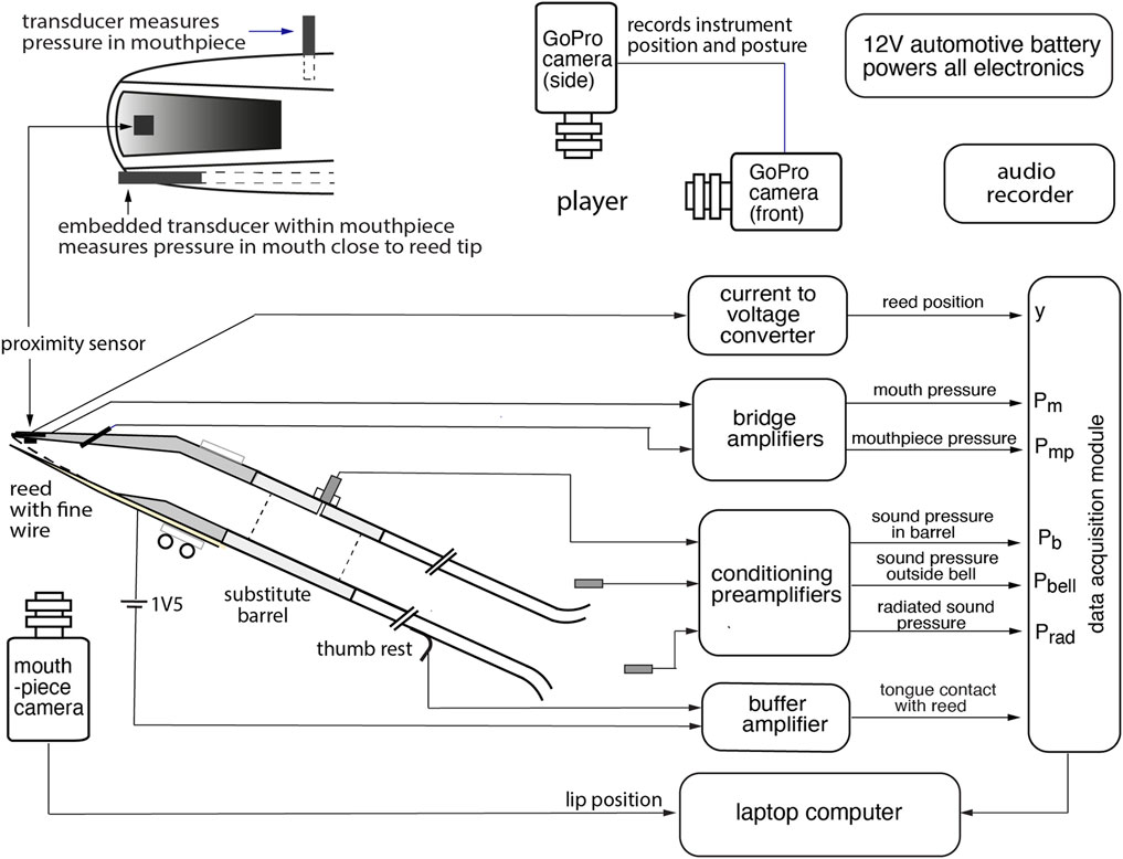
FIGURE 1. Schematic diagram (not to scale) of the overall measurement apparatus.

FIGURE 2

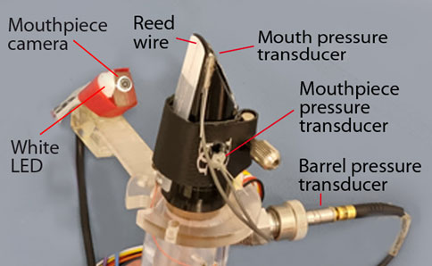
FIGURE 2. Detail of the mouthpiece with fitted sensors.

2.1 Modified clarinet with sensors

The modified clarinet mouthpiece and barrel fitted to the laboratory clarinet are illustrated schematically in Figure 1. A photograph of the mouthpiece in Figure 2 shows the most important sensors in the setup. The apparatus measures the following variables:

• Mouth pressure ($P_m$): A miniature pressure sensor (8507C-2, Endevco, Irvine, CA) is fitted into the corner of the mouthpiece so that its sensing membrane is exposed to the air inside the player’s mouth during playing. It is connected to a bridge amplifier (see schematics presented as Supplementary Material S1.

• Mouthpiece pressure ($P_{mp}$): A second miniature pressure sensor is fitted through a hole on the side of the mouthpiece, 30 mm away from the mouthpiece tip. It measures mouthpiece pressure at that point and is connected to a similar bridge amplifier. This measurement is affected by turbulence. In many of the uses of this signal, turbulence is not a major problem because it is averaged out during one window of sampling. For critical uses, the barrel pressure, which is much less affected by noise, can be used to estimate pressure at the tip of the mouthpiece, but this is beyond the scope of the current article.

• Reed position (y): A reflective, infrared proximity sensor (QRE1113, ON Semiconductor, Phoenix, AZ) is mounted inside the mouthpiece, 5 mm from the mouthpiece tip, directly opposite the reed. It is orientated to measure the displacement of the reed (with a minimum gap of 1 mm, achieved when the reed touches the lay and completely closes the mouthpiece). Its output is connected to a current-to-voltage converter (see schematics presented as Supplementary Material S1). A section of the flat side of the reed is painted matte white to increase diffuse reflection.

• Barrel sound pressure ($P_b$): A modified cylindrical barrel was made of plexiglass. A hole of 1 mm in diameter connects the inside bore of the barrel to a Swagelok adapter, 20.5 mm from the mouthpiece junction. This adapter holds a 1/4″ microphone (4944A, Brüel & Kjær, Næru, Denmark) connected to a conditioning preamplifier (Nexus 2690, Brüel & Kjær, Næru, Denmark) to provide calibrated gain. The embouchure camera is mounted on a frame attached to this barrel.

• Sound pressure outside bell ($P_{bell}$): A bracket attached to the bell holds a Brüel & Kjær 1/4″ microphone parallel to the instrument axis and directed towards the player. Not visible in Figure 2.

• Radiated sound pressure ($P_{rad}$): A 3/4″ microphone (RODE NT3, Sydney, Australia) mounted on a stand captures the sound radiated by the instrument. It is mounted at the same height as the bell and at a distance of 45 cm. Not visible in Figure 2.

• Tongue-reed contact: A thin (80 $\mu m$ diameter) wire is glued to the outer side of a synthetic reed (Légère Reeds, Barrie, Ontario) and insulated with varnish except for the final 2 mm from the tip of the reed. A small potential difference (1.5 V) is present between this wire and the thumb rest of the clarinet. Consequently, whenever the reed is tongued and the wire is touched by the tongue, a small current (∼1 µA) flows. This produces a voltage across a series resistor input to a buffer amplifier (see schematics in Supplementary Material S1).

The electronic signals from the above sensors are recorded at 51.2 kHz using a USB digital acquisition module (National Instruments DAQ 9234 and 9174) using the MATLAB DAQ toolbox. The DAQ system was chosen because a conventional audio interface is unable to capture the low-frequency components or DC offsets of some of the measurements, for instance, mouth pressure or reed displacement.

All measurements are made in a room designed to reduce background noise and reverberation. It has a reverberation time of no more than tens of milliseconds at the frequencies of interest.

For electrical safety, it is essential that the apparatus be completely isolated from the electrical mains supply. This is achieved by supplying all the electronics (i.e. Nexus conditioning preamplifier, digital acquisition module and custom electronics) from a 12 V automotive battery. The measurement computer (a laptop) runs from its internal battery during measurements.

To reduce the number of cables attached to the instrument, this version of the apparatus does not include key position sensors. We have studied key motion in detail previously (Almeida et al., 2009). For most purposes, the key motion is effectively binary and can be inferred from the note detected and/or the video (but see also Chen et al., 2009).

2.2 Relative position of player and instrument

2.2.1 Instrument motion

Two small video cameras (one GoPro 4 and one GoPro Hero 5, GoPro, San Mateo, CA) capture front and side views of the player and clarinet. The walls of the room and the clarinet are fitted with ArUco markers (Garrido-Jurado et al., 2014) as seen in Figure 3. These markers are analogous to QR codes that encode a single integer digit. They are easy to track with an automated tracking algorithm and can be uniquely identified in an image.

FIGURE 3

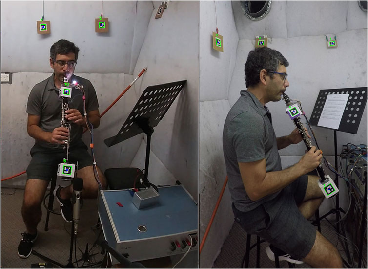
FIGURE 3. Synchronised capture of front and side views of player. Green rectangles show the detected ArUco markers tracking the motion of the clarinet.

2.2.2 Insertion of clarinet into mouth

One small endoscope camera (3.5 mm mini Android, GearBest, Guang Dong, China, hereafter called mouthpiece camera) is attached to a bracket mounted on the substitute barrel; it captures a side view of the clarinet mouthpiece. A coloured tag is glued to the side of the mouthpiece exposed to the camera, so that the position of the lip obscuring the tag can be tracked automatically in the video (see next section). The tag is illuminated by a white LED attached by a bracket to the substitute barrel. It can be seen in Figures 2, 3.

Videos with sound are recorded separately on each of the three cameras and synchronised later with the electronic signals using the audio fingerprinting tool described below.

2.3 Mouthpiece video analysis

The mouthpiece camera is attached to the clarinet barrel, about 60 mm from the mouthpiece. A sample frame captured by this camera is shown in Figure 4. Image analysis is performed using basic manipulation functions in the openCV library (Bradski, 2000) to determine how far the mouthpiece is inserted into the mouth.

FIGURE 4

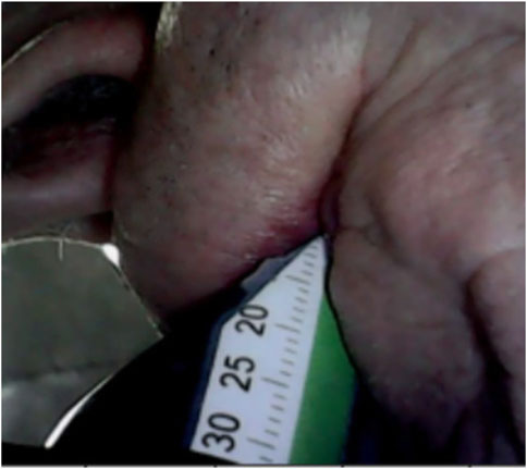
FIGURE 4. Sample frame from the mouthpiece camera during human performance. The mm scale and green target are glued to the clarinet mouthpiece.

Tracking involves identifying the green area in the scale and the target, which are both glued to the side of the mouthpiece, as shown in Figure 4. Identification of the green area is done by matching a range of Hue, Saturation, and Value. The narrowest range is matched on hue, as this is the most stable of the three colour variables when there are changes in lighting and orientation.

Although the camera is attached to the instrument, the support is not completely rigid, and the position of the scale on the frame can change with the movements of the clarinet. Because of this, the numbers on the scale are tracked for the length of the recording. The tracking is done using both an optical flow algorithm (precise to better than one pixel because it averages the motion of multiple pixels) and template matching (precise to one pixel). A Kalman filter combines both trackers, also interpolating the position if either tracker fails.

2.4 Motion capture

Two views of the player are recorded using GoPro cameras (see frame grabs in Figure 3). The instrument is fitted with a set of unique markers (ArUco markers). These markers can usually be identified in each frame, allowing tracking of the motion of the clarinet. Each recognised marker in a frame is used as a template for template matching in the next frame using a correlation-based algorithm. This allows tracking of the marker position even if it is blurred by motion. A Kalman filter interpolates for the position whenever the tags are obscured.

Google MediaPipe is used as an approximate tracker for the player’s head, which allows the angle between the clarinet and the musician’s face to be approximately determined. Facial data are used in the example below to calculate the tilt angle of the instrument relative to the head.

3 Methods

A set of software tools was developed to process the recorded data as automatically as possible. Parts may be used in similar contexts, even independently of the measurement apparatus. We make them available in a dedicated repository on GitHub (https://github.com/goiosunsw/mipcat), with additional explanation and technical documentation. Data is processed according to the flowchart in Figure 5: first, all raw signals are synchronized from different devices; second, several meaningful time series are extracted from raw signals and from videos (to obtain the lip position at which the player bites the reed and motion of the clarinet); third, a semi-automated segmentation is run on one of the audio signals to label note boundaries; fourth, several descriptive statistics from the time series are calculated for each note using labelled note boundaries, and fifth, transients are detected for each note for calculating transient statistics.

FIGURE 5

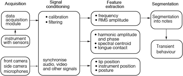
FIGURE 5. Flowchart of the software processing applied to the signals by MIPCAT. Acquired signals go through some pre-processing steps (conditioning), are processed to extract time-series of low-level sound features and are then segmented into notes and sub-segmented into transient and sustained portions.

3.1 Synchronisation of signals and video captures

All the signals from sensors are captured by a digital acquisition (DAQ) module and are thus synchronised with each other at acquisition time. Video signals from the general-purpose cameras are captured independently and thus require post-synchronisation. This is provided by comparing their audio signals with the audio signal from an external microphone captured by the DAQ unit using a fingerprinting algorithm (Cano et al., 2005). By doing this, the videos are synchronised with all the other signals captured by the DAQ module.

Synchronisation of two signals is usually achieved by finding the delay between two signals. The fingerprint of each audio signal is based on the peak bins of each spectrogram (FFT window size: 1,024 samples, i.e. 20 ms). The algorithm then matches peak pairs in the source signal with peak pairs in the reference signal according to their frequencies and time difference. For each matching peak pair, the delay between the peak pair in the reference signal and its corresponding pair in the target signal is recorded. When running through both signals, the distribution of the delays between matching pairs will exhibit a maximum value corresponding to the true delay between the two signals.

3.2 Time series calculation

Several time series are calculated from the raw signals:

• Fundamental frequency $f_0$: This is calculated from the chosen signal using the Yin algorithm implemented in librosa (https://librosa.org), a Python library for audio analysis, producing a time series of fundamental frequency values at a rate of 100 values per second.

• DC values of the mouth pressure and reed signals: A low pass filter with a cut-off frequency of 10 Hz is applied in the frequency domain.

• RMS amplitude of all pressure signals and the reed signal: Calculated as the standard deviation of the samples in a windowed portion of the signal. A Hann window is used and the value of the sum of the squared windowed signal is divided by the sum of the window so that the RMS value is correctly normalised. The window is 1,024 samples or 20 ms long.

• Spectral centroid of the pressure signals: Calculated from a spectrogram of the signals. Each frame is a Short-Time Fourier Transform and from it the centroid is calculated as the amplitude-weighted average of the bin frequencies.

• Harmonic amplitudes and phases: Pressure and reed signals are heterodyned with sinusoids (complex exponentials) at multiples of the fundamental frequency, and then summed over windows, as for the calculation of the RMS envelope. A complex time series is obtained, whose absolute value corresponds to the amplitude of the nth harmonic and whose phase is relative to the heterodyning sinusoid. This allows comparison of relative phases of different signals, for example the phase difference between the acoustic pressures measured in the mouth $P_m$ and mouthpiece $P_{mp}$ (which is usually close to, but not exactly, 180°).

Many other parameters could be calculated, including several related to timbre (roughness, sharpness, etc.). We chose to include only brightness and the first five harmonics here, as they are the ones that are easiest to relate to the player parameters. Figure 6 illustrates an example of these time-series with some of the subsequent processing described below.

FIGURE 6

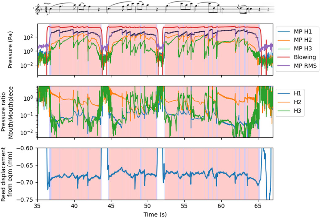
FIGURE 6. Example time-series extracted from a recording shown in the applications section (Section 4). The top graph shows the blowing pressure in pascals, the RMS amplitude of the pressure measured inside the mouthpiece, and the RMS amplitude of the first three harmonics (H1 to H3). The middle graph shows the ratios of the pressure of nth harmonic amplitude in the mouth to that in the mouthpiece. The bottom graph shows the average reed displacement from equilibrium (mm, negative values mean closer to the mouthpiece). The time axis is in seconds.

3.3 Semi-automated segmentation of time series at note level

The recordings are segmented at the level of individual notes using the frequency and amplitude time series extracted from one of the audio signals, the choice depending on the available channels in the setup. For the instrument used in the example below, the barrel signal is used because it is less affected by turbulence, and the fundamental of each note has a larger amplitude relative to higher harmonics, making automated extraction of fundamental frequency more reliable. For an instrument without fitted sensors, the signal from the radiated sound pressure microphone can be used.

The segmentation process starts by using the time series of fundamental frequency values at a rate of 100 values per second. This time series is smoothed using a median filter with a window length of 100 ms; this prevents short frequency changes due to wrong octave detections from being detected as very short notes. Frequency values are then quantized to an integral number of equal-tempered semitones, first with respect to a reference of 440 Hz for A4. A distribution of the deviations from integer semitones is calculated for each recording, and the average deviation is used to calculate a new reference value for A4 and to calculate a new set of integer pitch values.

An amplitude time series is also extracted as the RMS value of a windowed portion of the signal. Dips in the RMS amplitude that are larger than 3 dB are recorded as possible indicators of note boundaries, to be used later when aligning with a musical score. The segmentation into notes happens in two stages: The first stage uses the changes in pitch (as integer semitone values) and the dips in amplitude. In the examples shown here (Figure 7), amplitude dips that occur within 100 ms of a pitch change are interpreted as indicators of the same note boundary, because pitch change is usually accompanied by an amplitude dip.

FIGURE 7

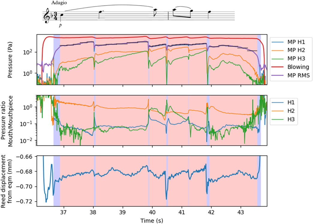
FIGURE 7. A 7-s sample from the applications section (Section 4), overlapping with the time period shown in Figure 6 on an expanded time scale showing six notes with segmentation boundaries (included in the white region), steady state region in red shading, and 5-segment envelope simplification for characterisation of each note. “Blowing” means the (DC or slowly varying) blowing pressure in the mouth, “MP” means mouthpiece, and H1 to H3 indicate fundamental and harmonics. Transient regions are marked as blue regions (see Figure 8).

On a second stage, the fundamental frequencies of the first-stage segmented notes are matched with the original score; this process is looped for a variable number of times. The number of repetitions is adjusted until the match is optimal; this reveals how many times the musical excerpt is played in a recording (how many recording “takes”). Notes that are unmatched and contiguous with a matched note having the same pitch are included with the matched note because they possibly indicate false detection of note change from an amplitude dip. From the second pass segmentation, a Praat (Boersma and Weenink, 2020) TextGrid file that labels all the detected note boundaries is produced; the note boundaries can be edited by hand to correct any boundaries placed incorrectly by the segmentation algorithm. In many cases no adjustment is required.

3.4 Note and excerpt descriptors

Descriptive statistics are gathered from the time series through the duration of the notes segmented, as described above. In general, central tendencies are extracted using the median value and a variability measure is assigned using the interquartile range.

Transients are detected in three steps (see Figure 8):

• The global maximum of the note envelope is found (blue vertical line).

• Envelope minima before and after the note are found as the global minimum between two consecutive notes (green vertical lines).

• One of two lines of constant slope (dashed blue lines) is subtracted from the envelope. Maxima in this function are found between the boundaries found in steps 1 and 2 for attack and release corners. Subtraction of lines with positive and negative slopes ensures that a maximum is found near the beginning or end of the note, respectively. The slope of the line subtracted for the attack is +40 dB/s and that for the release is −80 dB/s. These values, found by manually testing on a dozen examples, are a compromise between minimum typical attack slopes and maximum slopes in the bulk of the note.

FIGURE 8

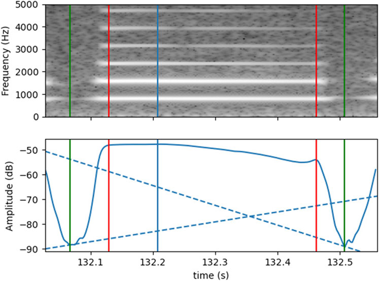
FIGURE 8. Transient detection steps exemplified for a single note. Top: spectrogram, bottom: amplitude envelope (solid blue line). Dashed lines indicate the slopes subtracted from the envelope in order to find corner positions (red) which are maxima of the subtracted signal. Note boundaries (green) are detected from the minima before the corner point. Note that for this moderately high note, the even harmonics are not weak.

This method is relatively robust for the detection of starting transients (attacks) but less so for end note transients, which can have much larger variations in shape.

4 Empirical application

4.1 Background

We applied MIPCAT to examine and compare measurements from two expert (professional) clarinettists and an amateur each playing a short excerpt of music from the classical repertoire, using the laboratory instrument and apparatus. The apparatus outputs showed what physical variable control was used to achieve their musical aims; this allowed us to compare different performances of the same piece.

In this sample study, a few variables that seem important to characterise a musical interpretation are selected. Some audio features (fundamental frequency and amplitude) are common to many instruments. Blowing pressure and reed position are two fundamental parameters in a physical model of a clarinet. Finally, visual parameters extracted from the videos are important in a multimodal setting.

Two professional musicians were engaged to play short music excerpts as samples for a practical test of the equipment’s functionality. Both players have held positions with leading national orchestras and have extensive solo experience nationally and internationally. The amateur player was part of the research team and had 4 years’ experience playing the clarinet.

The players were asked to play an excerpt (see Figure 9) from the second Movement of Wolfgang Amadeus Mozart’s Clarinet Concerto K. 622. They played the sample twice using the same, sensor-fitted instrument. The repetition was done shortly after the first performance, with a short break (whose duration was not stipulated).

FIGURE 9

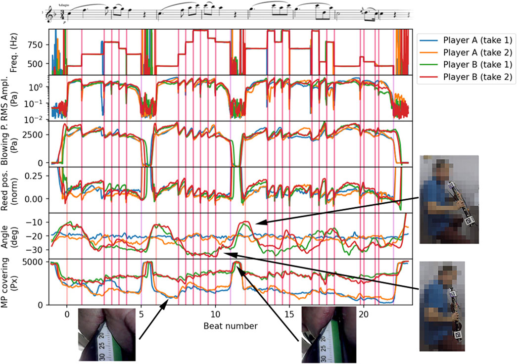
FIGURE 9. Example data from two expert clarinettists playing an excerpt from Mozart’s Clarinet Concerto (two takes by each player). Images are pixelated to preserve player anonymity. The top two graphs show the fundamental frequency in Hz and the RMS amplitude of the sound inside the mouthpiece in pascals. The third shows the blowing pressure inside the mouth, measured in pascals. The fourth shows the DC component of the normalised distance between reed and mouthpiece with a larger value indicating a larger aperture. The fifth shows the relative angle between the head and the instrument, in degrees. The sixth shows the amount of mouthpiece (MP) covered by the lips i.e., the unobscured green area in pixels, indicating lip position.

4.2 Results

Time series data from four performances are shown in Figure 9, showing two takes from each of two professional clarinettists. The time series extracted from the sensors and the cameras are aligned note by note: for every note, time is stretched or compressed linearly in one of the recordings to keep the note boundaries aligned with a steady metronome, corresponding to the number of beats from the beginning of the excerpt.

The output of the reed sensor changes for different reeds and for the different reed positions that result when players adjust the mouthpiece to their satisfaction. For this reason, the values in this time-series are normalised so that 0 corresponds to the closed reed, and 1 to the rest position.

Visual inspection of the MIPCAT outputs can also be used to compare the amateur player against the two professionals for the same excerpt discussed above. Apart from obvious note misses seen in the top panels (third and second last note of the extract), Figure 10 shows that for this amateur player, the amplitude of the notes varies less than that of the experts, and in different ways.

FIGURE 10

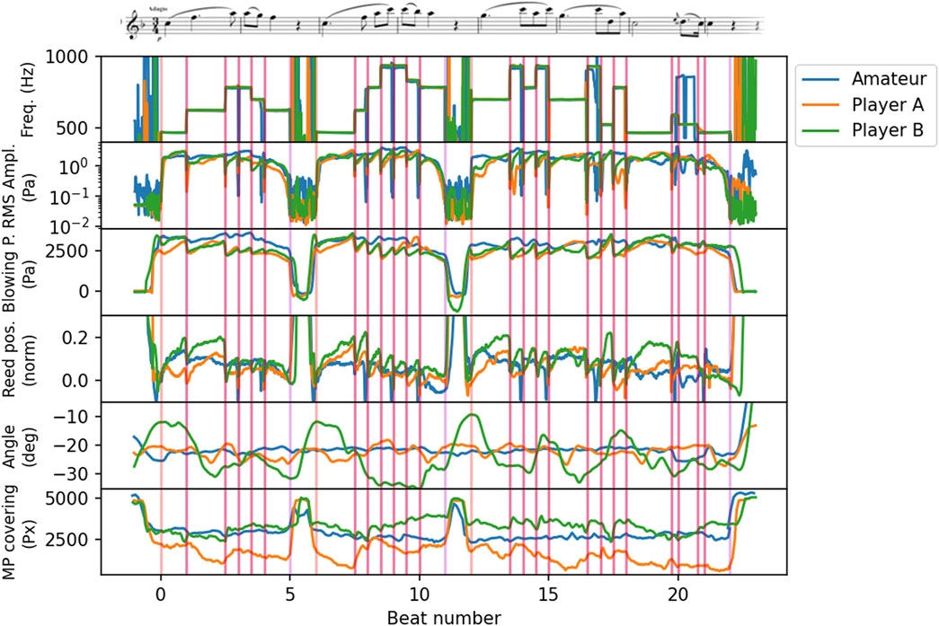
FIGURE 10. Comparison of excerpts played by three different players, including one amateur player. Such plots allow the identification of notable differences between an amateur player and a pair of expert, professional players.

There are audible differences in the sound produced by the two expert players and larger differences between the amateur and the experts. The musical ‘shape’ of the phrases is indicated by amplitude; the amplitude envelopes are also different for some notes. These differences are not always easy to relate to measured player variables, though the differences in the rise in blowing pressure and note amplitude throughout the longer notes are systematic. Further, the systematic amplitude differences when two expert players play the same note (Figure 11 are accompanied by systematic differences in blowing pressure).

FIGURE 11

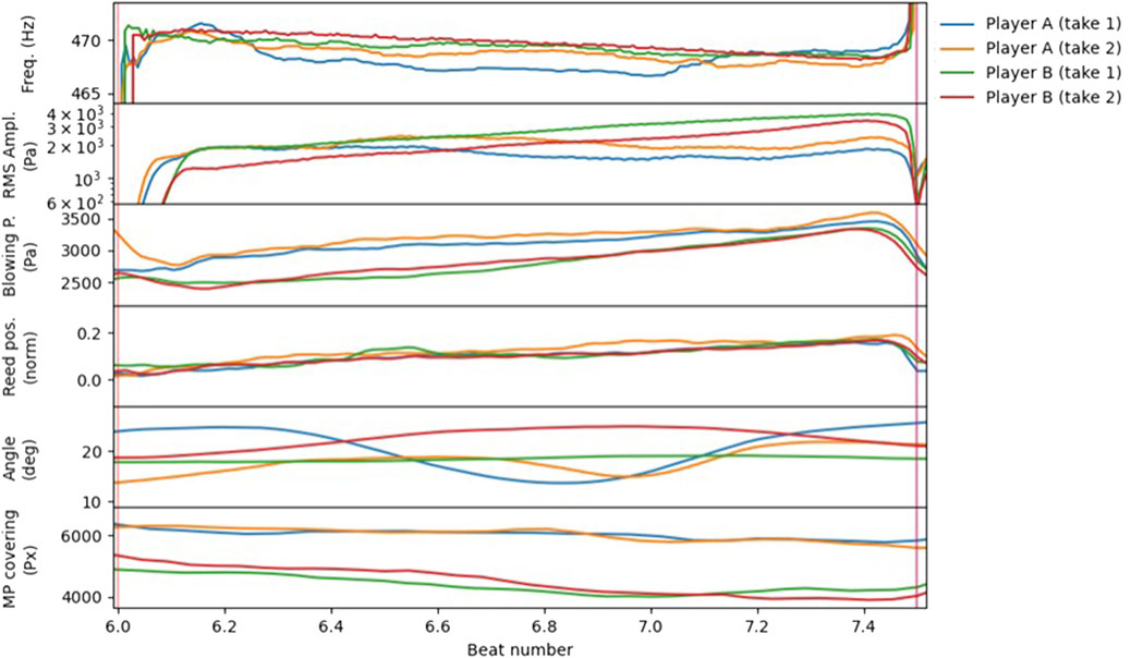
FIGURE 11. One note from Figure 8 shown on an expanded time scale.

It is interesting to note also how expert player B produces less motion with the clarinet than player A, even though the plots of the amplitude envelope appear—to the eye—very similar (Figure 9). Player B keeps the bite position relatively constant; in contrast, player A varies it during these phrases. This is interesting because teachers disagree on whether one should aim to keep a ‘fixed bite’, or whether it is an acceptable control variable for expression (Almeida et al., 2022). The DC reed position is an indicator of bite force (a larger bite force produces smaller aperture).

4.3 Discussion

With researchers running the current prototype toolbox, the outputs from MIPCAT could be applied in several ways. The data can be used to model the physical parameters involved in playing—for example the ideal approach taken by professional players, and to relate these to the corresponding musical characteristics, and even the affective intentions of the player and responses of the listener. Further nuanced applications could involve examining how different performer approaches can be traced back to their physical parameter origins. MIPCAT can also be used by clarinet teachers and students for pedagogical purposes. For example, a database of excerpts played by expert players would provide a set of good quality performances where the different solutions they each impart can be examined in a novel, high precision setting. Student performances could then be compared to these performances and notable differences identified and addressed at the level of physical interaction with the clarinet, rather than, or in addition to more abstract descriptions of how to play.

5 Conclusion

The MIPCAT system reported here measures player-controlled variables, including blowing pressure, tongue-reed contact, sound pressures in the mouth and instrument, details of the embouchure, and the position in which the instrument is held. These and the output sound are recorded. A suite of software tools extract features from the time-course of these variables. This rich set of audio, visual and player-control features allows more detailed and quantitative study on music performance, opening a range of possibilities for music performance research and pedagogy. This study demonstrates how MIPCAT could be applied to provide new insights into relations among variables in the sound and the simultaneously occurring physical aspects of playing that have not previously been available to the research community. This are likely to lead to increased understanding of performance nuance that has applications for music pedagogy and psychology. For example, students could use MIPCAT to visualise both audio and player-control parameters in a quantitative way and compare their performances with those by expert players; students could also learn how to better convey different emotions in music performances.

Although MIPCAT was here applied to clarinet playing, it (or parts of it) could be easily adapted to other reed instruments, or to other families of instruments. Future improvements of the toolbox could include modularising different parts of the MIPCAT toolbox so that each module is more independent and adaptable to other instruments.

Data availability statement

The datasets presented in this study can be found in online repositories. The names of the repository/repositories and accession number(s) can be found below: https://doi.org/10.5281/zenodo.7042527.

Ethics statement

The studies involving human participants were reviewed and approved by UNSW Australia Human Research Ethics Advisory Panel. The patients/participants provided their written informed consent to participate in this study. Written informed consent was obtained from the individual(s) for the publication of any potentially identifiable images or data included in this article. The demonstrator in Figure 3 is a member of the team and has consented to have his picture published.

Author contributions

Hardware and software components of the MIPCAT were developed by AA, WL, and JS. All the authors participated in the experimental design and the production of this manuscript.

Funding

This study is funded by the Australian Research Council (DP200100963).

Acknowledgments

The authors wish to thank all the musicians that participated in fine-tuning the method and obtaining example results. We warmly thank the Australian Research Council for their support of this project, Yamaha for the clarinet and Légère for the reeds used in this project. It was conducted on Bedegal country.

Conflict of interest

The authors declare that the research was conducted in the absence of any commercial or financial relationships that could be construed as a potential conflict of interest.

Publisher’s note

All claims expressed in this article are solely those of the authors and do not necessarily represent those of their affiliated organizations, or those of the publisher, the editors and the reviewers. Any product that may be evaluated in this article, or claim that may be made by its manufacturer, is not guaranteed or endorsed by the publisher.

Supplementary material

The Supplementary Material for this article can be found online at: https://www.frontiersin.org/articles/10.3389/frsip.2023.1089366/full#supplementary-material

References

Almeida, A., Chow, R., Smith, J., and Wolfe, J. (2009). The kinetics and acoustics of fingering and note transitions on the flute. J. Acoust. Soc. Am. 126 (3), 1521–1529. doi:10.1121/1.3179674

PubMed Abstract | CrossRef Full Text | Google Scholar

Almeida, A., George, D., Smith, J., and Wolfe, J. (2013). The clarinet: How blowing pressure, lip force, lip position and reed "hardness" affect pitch, sound level, and spectrum. J. Acoust. Soc. Am. 134 (3), 2247–2255. doi:10.1121/1.4816538

PubMed Abstract | CrossRef Full Text | Google Scholar

Almeida, A., Li, W., Schubert, E., Smith, J., and Wolfe, J. (2022). Expressive goals for performing musicians: The case of clarinetists. Thousand Oaks, CA: Musicae Scientiae. doi:10.1177/10298649221122155

CrossRef Full Text | Google Scholar

Boersma, P., and Weenink, D. (2020). Praat: Doing phonetics by computer [computer program] version 6.1.10. retrieved 23 March 2020.

Google Scholar

Bradski, G. (2000). The OpenCV library. Dr. Dobb's Journal of Software Tools.

Google Scholar

Bresin, R., and Umberto Battel, G. (2000). Articulation strategies in expressive piano performance analysis of legato, staccato, and repeated notes in performances of the andante movement of Mozart’s sonata in g major (k 545). J. New Music Res. 29 (3), 211–224. doi:10.1076/jnmr.29.3.211.3092

CrossRef Full Text | Google Scholar

Camurri, A., Coletta, P., Varni, G., and Ghisio, S. (2007). “Developing multimodal interactive systems with EyesWeb XMI,” in Proceedings of the 7th international conference on new interfaces for musical expression (NIME ’07), New York, NY.

CrossRef Full Text | Google Scholar

Camurri, A., Mazzarino, B., Ricchetti, M., Timmers, R., and Volpe, G. (2004). Multimodal analysis of expressive gesture in music and dance performances. Lect. Notes Comput. Sci. doi:10.1007/978-3-540-24598-8_3

CrossRef Full Text | Google Scholar

Camurri, A., Volpe, G., De Poli, G., and Leman, M. (2005). Communicating expressiveness and affect in multimodal interactive systems. IEEE Multimed. 12 (1), 43–53. doi:10.1109/MMUL.2005.2

CrossRef Full Text | Google Scholar

Cano, P., Batlle, E., Gómez, E., deGomes, C. T. L., and Bonnet, M. (2005). “Audio fingerprinting: Concepts and applications,” in Computational intelligence for modelling and prediction. Editors S. K. Halgamuge, and L. Wang (Germany: Springer), 233–245.

CrossRef Full Text | Google Scholar

Caramiaux, B., Wanderley, M. M., and Bevilacqua, F. (2012). Segmenting and parsing instrumentalists' gestures. J. New Music Res. 41 (1), 13–29. doi:10.1080/09298215.2011.643314

CrossRef Full Text | Google Scholar

Caussé, R. E., Noisternig, M., and Warusfel, O. (2015). Sound radiation properties of musical instruments and their importance for performance spaces, room acoustics measurements or simulations, and three-dimensional audio applications. J. Acoust. Soc. Am. 138, 3. doi:10.1121/1.4933653

CrossRef Full Text | Google Scholar

Chadefaux, D., Le Carrou, J.-L., Fabre, B., and Daudet, L. (2012). Experimentally based description of harp plucking. J. Acoust. Soc. Am. 131 (1), 844–855. doi:10.1121/1.3651246

PubMed Abstract | CrossRef Full Text | Google Scholar

Chatziioannou, V., and Hofmann, A. (2015). Physics-based analysis of articulatory player actions in single-reed woodwind instruments. Acta Acustica united Acustica 101 (2), 292–299. doi:10.3813/AAA.918827

CrossRef Full Text | Google Scholar

Chen, J.-M., Smith, J., and Wolfe, J. (2009). Pitch bending and glissandi on the clarinet: Roles of the vocal tract and partial tone hole closure. J. Acoust. Soc. Am. 126 (3), 1511–1520. doi:10.1121/1.3177269

PubMed Abstract | CrossRef Full Text | Google Scholar

Ferguson, S., Schubert, E., and Stevens, C. J. (2014). “Dynamic dance warping: Using dynamic time warping to compare dance movement performed under different conditions,” in Proceedings of MOCO ’14: International Workshop on Movement and Computing. Editors F. Bevilacqua, S. F. Alaoui, J. Françoise, P. Pasquier, and T. Schiphorst (Association for Computing Machinery), 94–99. doi:10.1145/2617995.2618012

CrossRef Full Text | Google Scholar

Fréour, V., and Scavone, G. P. (2013). Acoustical interaction between vibrating lips, downstream air column, and upstream airways in trombone performance. J. Acoust. Soc. Am. 134 (5), 3887–3898. doi:10.1121/1.4823847

PubMed Abstract | CrossRef Full Text | Google Scholar

Furuya, S., and Soechting, J. F. (2012). Speed invariance of independent control of finger movements in pianists. J. Neurophysiology 108 (7), 2060–2068. doi:10.1152/jn.00378.2012

PubMed Abstract | CrossRef Full Text | Google Scholar

Garrido-Jurado, S., Muñoz-Salinas, R., Madrid-Cuevas, F. J., and Marín-Jiménez, M. J. (2014). Automatic generation and detection of highly reliable fiducial markers under occlusion. Pattern Recognit. 47 (6), 2280–2292. doi:10.1016/j.patcog.2014.01.005

CrossRef Full Text | Google Scholar

Goebl, W., and Palmer, C. (2008). Tactile feedback and timing accuracy in piano performance. Exp. Brain Res. 186 (3), 471–479. doi:10.1007/s00221-007-1252-1

PubMed Abstract | CrossRef Full Text | Google Scholar

Guillemain, P., Vergez, C., Ferrand, D., and Farcy, A. (2010). An instrumented saxophone mouthpiece and its use to understand how an experienced musician plays. Acta Acustica united Acustica 96 (4), 622–634. doi:10.3813/AAA.918317

CrossRef Full Text | Google Scholar

Hofmann, A., and Goebl, W. (2016). Finger forces in clarinet playing. Front. Psychol. 7, 1140. doi:10.3389/fpsyg.2016.01140

PubMed Abstract | CrossRef Full Text | Google Scholar

Jensenius, A. R. (2018). “Methods for studying music-related body motion,” in Springer handbook of systematic musicology. Editor R. Bader (Germany: Springer), 805–818.

CrossRef Full Text | Google Scholar

Jensenius, A. R. (2006). “Using motiongrams in the study of musical gestures,” in Proceedings of the International Computer Music Conference (New Orleans, LA: Tulane University), 499–502.

Google Scholar

Leman, M., Maes, P.-J., Nijs, L., and Van Dyck, E. (2018). “What is embodied music cognition?,” in Springer handbook of systematic musicology. Editor R. Bader (Germany: Springer), 747–760.

CrossRef Full Text | Google Scholar

Li, W., Almeida, A., Smith, J., and Wolfe, J. (2016b). How clarinettists articulate: The effect of blowing pressure and tonguing on initial and final transients. J. Acoust. Soc. Am. 139 (2), 825–838. doi:10.1121/1.4941660

PubMed Abstract | CrossRef Full Text | Google Scholar

Li, W., Almeida, A., Smith, J., and Wolfe, J. (2016a). The effect of blowing pressure, lip force and tonguing on transients: A study using a clarinet-playing machine. J. Acoust. Soc. Am. 140 (2), 1089–1100. doi:10.1121/1.4960594

PubMed Abstract | CrossRef Full Text | Google Scholar

Meyer, J. (2009). Acoustics and the performance of music: Manual for acousticians, audio engineers, musicians, architects and musical instrument makers. Berlin: Springer Science and Business Media.

Google Scholar

Palmer, C., Koopmans, E., Loehr, J. D., and Carter, C. (2009). Movement-related feedback and temporal accuracy in clarinet performance. Music Percept. 26 (5), 439–449. doi:10.1525/mp.2009.26.5.439

CrossRef Full Text | Google Scholar

Pamiès-Vila, M. (2021). Expressive performance on single-reed woodwind instruments: An experimental characterisation of articulatory actions [doctoral dissertation. Vienna: University of Music and Performing Arts.

Google Scholar

Pàmies-Vilà, M., Hofmann, A., and Chatziioannou, V. (2018). Analysis of tonguing and blowing actions during clarinet performance. Front. Psychol. 9, 617. doi:10.3389/fpsyg.2018.00617

PubMed Abstract | CrossRef Full Text | Google Scholar

Pavlidou, M. (1997). A physical model of the string-finger interaction on the classical guitar. Cardiff: Ph.D., University of Wales.

Google Scholar

Repp, B. H. (1995). Acoustics, perception, and production of legato articulation on a digital piano. J. Acoust. Soc. Am. 97 (6), 3862–3874. doi:10.1121/1.413065

PubMed Abstract | CrossRef Full Text | Google Scholar

Scavone, G. P., Lefebvre, A., and da Silva, A. R. (2008). Measurement of vocal-tract influence during saxophone performance. J. Acoust. Soc. Am. 123 (4), 2391–2400. doi:10.1121/1.2839900

PubMed Abstract | CrossRef Full Text | Google Scholar

Schoonderwaldt, E., Demoucron, M., and Rasamimanana, N. (2008). A setup for measurement of bowing parameters in bowed-string instrument performance. J. Acoust. Soc. Am. 123 (5), 3664. doi:10.1121/1.2934989

CrossRef Full Text | Google Scholar

Wanderley, M. M., Vines, B. W., Middleton, N., McKay, C., and Hatch, W. (2005). The musical significance of clarinetists' ancillary gestures: An exploration of the field. J. New Music Res. 34 (1), 97–113. doi:10.1080/09298210500124208

CrossRef Full Text | Google Scholar