Apparent color picker: color prediction model to extract apparent color in photos

1 Introduction

Color pickers and selectors are utilized to extract preferable colors from images, videos, and objects. These tools are popular interfaces in the fields of design and art. The selected colors are reused in illustrations and graphs (Ryokai et al., 2004; Shugrina et al., 2017). Other color picker and selector applications include map coloring (Harrower and Brewer, 2003), architectural paint selection (Bailey et al., 2003), cosmetics selection (Jain et al., 2008), and color testing of chemicals (Solmaz et al., 2018). For extracting the preferable color of the users, it is essential to consider users’ color perception.

Various factors influence color perception, often resulting in the difference between pixel-wise color and the apparent color. These factors include color constancy, adjacent colors, illumination, and context. Color constancy is related to the ability to achieve stable color perception regardless of changes in the visual environment, such as illumination, the presence of shadows, and the biased color of lighting (Ebner, 2012). The additional effects of adjacent colors are known as the simultaneous contrast (Wong, 2010; Klauke and Wachtler, 2015) and assimilation effects (Anderson, 1997). Based on psychophysical experiments in various lighting environments (Kuriki and Uchikawa, 1996; Granzier and Gegenfurtner, 2012), a color appearance model (CAM) (Moroney et al., 2002; Luo and Pointer, 2018) and S-CIE Lab model (Johnson and Fairchild, 2003) have been proposed to correct these effects.

However, no methodology relating to factors other than color temperature and illumination has been proposed to correct the discrepancy between the apparent and pixel colors. Notably, conventional studies have not constructed a model estimating the apparent color in photographs. For example, several studies proposed correction methods for unbalanced lighting images (Agarwal et al., 2007; Gijsenij et al., 2011; Akbarinia and Parraga, 2017; Wang et al., 2017). Recently, color correction algorithms have been capable of handling multiple illumination (Hussain et al., 2019; Akazawa et al., 2022; Vršnak et al., 2023) and image sequences (Qian et al., 2017; Zini et al., 2022); they did not consider human perception. It is known that humans have imperfect color constancy, and the apparent color does not always match the corrected color in the reference light source (Kuriki and Uchikawa, 1996). Conventional color correction algorithms, including CAM, also do not consider the applications for the interface of extracting the apparent color in the same device. Other studies solved the problem of transferring colors that preserves color harmony; however, they did not consider human color perception in photographs (Cohen-Or et al., 2006; Reinhard et al., 2001; Zhang et al., 2013).

Therefore, in this paper, the authors investigate the suitable model structure and features for constructing an apparent color picker that extracts the apparent colors in photographs. Based on the apparent color dataset collected on psychophysical experiments, the authors construct regression models for predicting the apparent color from image features. Then, several models and image features are compared to select the suitable model and features that predict the apparent colors in photographs. Subsequent evaluation experiments with participants are conducted with two sets of images: a texture-based dataset (DTD dataset) and a landscape-based dataset (Places dataset). The prediction performance is evaluated by the ratio of colors output closer to the apparent than the pixel color. In summary, the main contributions of this paper are as follows:

• The authors constructed the regression model to predict the apparent colors in natural photographs. This model can be applied to the apparent color picker, thereby, extracting the color as users perceive.

• The authors confirmed the prediction performance of the proposed model for both a texture-based and a landscape-based dataset.

2 Materials and methods

2.1 Related work

2.1.1 Color perception and color appearance models

Color constancy is a phenomenon in which the perceived color of objects under various illuminations is relatively constant. For example, a red apple’s color is perceived as reddish, even under bluish illumination. The ability of color constancy improves when adding small amounts of full-spectrum illumination (Boynton and Purl, 1989). In addition to the characteristics of the light source itself, various factors affect color constancy. Previous studies have shown that color constancy is affected by whether the object is observed on a monitor or paper (Granzier et al., 2009), and whether the object is perceived as a surface or an illuminant color (Kuriki, 2015; Zhai and Luo, 2018). Other studies have reported that color constancy changes depending on whether a subject responds to the apparent or object color (Kuriki and Uchikawa, 1996), and whether they were asked to observe a 3D object or 2D image (Hedrich et al., 2009). Additionally, color constancy produced the remarkable illusion of “♯The Dress,” in which the observers of this specific image disagreed whether the dress color was black and blue or white and gold (Dixon and Shapiro, 2017; Lafer-Sousa and Conway, 2017).

Color perception is also affected by adjacent colors (Wong, 2010). The apparent color varies with the luminance and hue of the surrounding colors. Klauke et al. measured the changes in the apparent color induced in the different hues of its surroundings (Klauke and Wachtler, 2015). They found that the most significant perceived deviation in the induced color occurred when the difference between the stimulus and surrounding hues was about 45°. Additionally, Shapiro and Dixon et al. described the luminance illusions related to adjacent colors with a high-pass filter, reducing the effect of illuminations and shadows (Shapiro and Lu, 2011; Dixon and Shapiro, 2017; Shapiro et al., 2018). These illusions were also described and evaluated using machine learning models trained on natural images (Gomez-Villa et al., 2020; Hirsch and Tal, 2020; Kubota et al., 2021).

CAMs were proposed to grasp these perceptual characteristics. These are device-independent color models rather than a device-dependent color spaces, such as sRGB (Anderson et al., 1996). The models provide similar image appearance on different devices. CAM02 is a typical model of CAMs (Moroney et al., 2002). The color calculation of CAM02 requires the device’s luminance, white point’s XYZ value, and target’s XYZ value as input, and several color appearance parameters are obtained from the model. Several models including CAM02 for high luminance (Kim et al., 2009) and CAM16 (Luo and Pointer, 2018) were implemented as an extension of this model.

Although these CAMs can estimate the apparent color independent of the display devices, they cannot be directly adopted to construct the apparent color picker. This is because the models do not assume the tasks of extracting apparent colors in the same device and the effects of adjacent colors.

2.1.2 Color correction algorithms

Several color correction algorithms have been created to correct the white balance of color-biased images or to estimate illuminant color in images (Gijsenij et al., 2011). Color correction models can be broadly divided into feature-based and learning-based methods. Feature-based methods can formulate image transformations independently of the data, whereas learning-based methods have the advantage of dealing with more complex illumination environments. Feature-based methods include classical methods, such as gray-world and white-patch models, ridge regression (Agarwal et al., 2007), the difference of Gaussians (DoG) model (Akbarinia and Parraga, 2017), spatial frequency distribution (Cheng et al., 2014), Bayesian correlation estimation (Finlayson and Hordley, 2001), and achromatic point shift (Kuriki, 2018). The algorithms using convolutional neural network (CNN) (Barron, 2015; Wang et al., 2017), variational technique (Bertalmío et al., 2007), and generative adversarial network (GAN) (Sidorov, 2019) have been proposed as learning-based methods. Recent studies tackled more complicated issues, including multiple illumination estimation and correction with image sequences. Color correction algorithms for photographs containing multiple illumination sources were implemented using histogram features (Hussain et al., 2019), block-wise estimation (Akazawa et al., 2022), and deep learning models (Vršnak et al., 2023) to segment regions illuminated by a specific illuminant source. Illumination estimation for image sequences has also been performed using various strategies, including a recurrent deep network (Qian et al., 2017) and multilayer perceptron (Zini et al., 2022).

However, unlike human perception, these methods assume perfect color constancy. Humans have imperfect surface color constancy (Kuriki and Uchikawa, 1996) and may perceive different colors from the perfect white-balanced colors. Higher-order biases in human color perception would also affect the apparent color of users.

2.1.3 Color picker as an interactive interface

Colors are usually represented by points in a three-dimensional space, such as RGB, HSV, or L*a*b* color space. Thus, allowing the users to select these three-dimensional points is essential while reducing the operation loads on the color selection. There are two possible implementations for solving the problem: one is to support the user’s color selection by returning appropriate feedback, and the other is to automate parts of the selection process. Regarding the former, Douglas and Kirkpatrick reported that visual feedback affects the color extraction’s accuracy (Douglas and Kirkpatrick, 1999). Various methodologies have been developed to replace traditional color extraction interfaces, including the 3D color picker (Wu and Takatsuka, 2005), the Munsell color palette (MacEachren et al., 2001), and the touch panel-based color picker (Ebbinason and Kanna, 2014). In addition to the rule-based color extractors (Meier et al., 2004; Wijffelaars et al., 2008), a data-driven method using a variational autoencoder (VAE) (Yuan et al., 2021) has been proposed as a valid candidate for automated color selection models. Furthermore, examples of tools to automate color selection for data visualization include color selection based on spatial frequency and data types (Bergman et al., 1995), and constraints in the previously selected colors (Sandnes and Zhao, 2015).

Various interactive tools have also been implemented to select the preferable color from images and create a customized color palette. Shugrina et al. developed an interactive tool for artists to select customized color themes and mixed colors (Shugrina et al., 2017; Shugrina et al., 2019). Okabe et al. proposed an interface to design preferable illumination in the images (Okabe et al., 2007). The I/O Brush that extracts colors from physical objects is utilized to pick up from actual objects and draw with it (Ryokai et al., 2004).

However, these studies do not consider human color perception that are biased in both the pixel-wise color and the perfect white-balanced colors. This research aims to construct the regression model that predicts the users’ apparent colors in natural photographs based on a psychophysical dataset named an apparent color dataset (Kubota et al., 2022). Note that the main focus of this paper is prediction model construction and evaluation, which differs from the purpose of the previous paper, which focused on dataset construction and its analysis. The authors’ previous paper only collected and evaluated the apparent color datasets for photographs. Namely, the previous paper handled neither the construction of the regression model and features nor the experimental evaluation of the system performance.

2.2 Model selection from apparent color dataset

This section describes model construction and selection for creating the apparent color picker. First, the candidate features and model structures are described. Then, the color prediction performance is evaluated through trained models, which have various features and model structures. Based on the evaluation from these experiments, the authors select the suitable model and features for constructing the apparent color picker. Figure 1 shows the model structure adopted in this paper.

FIGURE 1

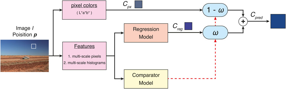
FIGURE 1. Model structure of the apparent color picker. From a given image I and selected position p, the features were extracted as multi-scale pixels or histograms. The regression model predicted the apparent color in the photos from the features. After the prediction, the comparator model weighed the pixel color C_px and the predicted color C_pred with the probability ω of whether the difference between the apparent color and pixel color was less than ΔE₀₀ = 5.0.

2.2.1 Candidate features and models

Several factors, including surrounding colors and biased illumination of images, influence the apparent color. It is necessary to select appropriate features and models to predict the apparent color from a given image. The following candidate features (the bottom red box in Figure 1) incorporate the surrounding color’s influence and biased illumination.

1. Multi-scale L*a*b* pixels (px27 features): the image was scaled down on a 1/2^H scale, and the L*a*b* values for each scale at the position corresponding to the original pixel were collected as features. The features reflected the average surrounding colors of the extracted position. This paper adopted 27-dimensional features by adding the average color of the whole image to the features calculated with H = 8.

2. Multi-scale histogram of L*a*b* values (hist features): histograms of N_i px around the original pixel were collected with bin size b = 8. The histograms of the surrounding colors discretized by b steps for L*a*b* were recruited as features. In this paper, N_i = [8, 16, 32, 64, 128, 256, 0] is adopted. Note that N_i = 0 indicates that the features are constructed from the whole image’s histogram.

The L*a*b* color model domain constitutes a uniform color space based on human color perception, in contrast to the non-uniform color spaces of RGB and HSV, which are not tailored to human perception (Robertson, 1977). Consequently, it is suitable to employ the L*a*b* color model and DE2000 color difference metric for dealing with human perceptual responses. The authors posited that utilizing the L*a*b* color space for the regression model would facilitate the development of the color extraction system more closely aligned with the responses. Although comparable results might be obtained through features within the HSV or RGB color domains, the authors did not conduct a direct comparisons between these alternatives.

The apparent color picker was constructed as a regression model (the orange box in Figure 1) that predicted the apparent color as a continuous L*a*b* value from the input features. As candidates for the model structure, the authors selected six model structures: linear regression (LR), ridge regression (RR), lasso (Lasso), support vector machine (SVM), random forest regression (RFR), and gradient boosting regression (GBR). Given the relatively modest volume of training data, the risk of overfitting in deep learning-centric models was deemed substantial. Thus, deep learning models are not employed in this paper.

Based on the performance evaluation results described in the next section, a comparator was employed to improve the predicted values. The comparator (the yellow box in Figure 1) was introduced to suppress the deterioration of predictions when there was a slight difference between apparent color and pixel color. The classifier determined the probability ω of whether the apparent color and pixel color difference from feature vectors is less than ΔE₀₀ = 5.0. After the classification, the weighted prediction value was calculated as C_pred = ω ⋅ C_reg + (1 − ω) ⋅ C_px. The random forest classifier (RFC) was employed in this paper.

2.2.2 Performance evaluation

The apparent color dataset (Kubota et al., 2022) was utilized for training the proposed model. The dataset consists of 1,100 photographs, each annotated with the apparent color using the adjustment method with a color palette. Each data entry has information, including the participant number, the image, the position to be responded, and the apparent color response. From these properties, the model utilized the image’s information, the position to be responded to and the apparent color response to calculate features from the input image. The features mentioned above were calculated from a given image and a position to be responded to input to the regression model as shown in Figure 1. Note that the output results in Sections 2.2.2.1–2.2.2.3 were calculated without a comparator to compare the performance of the candidate models and features independent of the comparator.

First, 80% (880 data) of the 1,100 data entries in the apparent color dataset were divided into training data and 20% (220 data) into validation data. The models were trained to predict the apparent color from feature vectors. To eliminate the effect of splitting the data into training and validation data, splitting the data was randomized with 100 different random numbers. The results of models trained on 100 different combinations of training data were averaged. The total results of this evaluation contained 88,000 items for the training data and 22,000 items for the validation data. The difference between the predicted and apparent colors was measured with the DE2000 metric (Sharma et al., 2005). Specifically, the prediction performance was compared in view of the following four points:

1. Model structure: to identify the appropriate regression model structure, the authors compared the prediction color of the six models described above. In this model selection, px27 features were adopted as feature vectors, and no restrictions for data range were imposed.

2. Feature types: to identify the appropriate features, the authors compared four features (the original pixel values only (px3), multi-scale pixel values (px27), histogram values (hist), and both multi-scale pixel values and histograms (px_hist)). In this feature selection, the LR and RFR models were adopted as the evaluation models, and no restrictions for data range were imposed.

3. Maximum values: to identify the appropriate range of training data, the authors compared the data range of color difference for training data. Only the items in the apparent color dataset satisfying the restriction with the DE2000 threshold ΔE₀₀ < c_th(c_th = 5.0, 10.0, 20.0, 30.0, all) were adopted as training data. The models were trained with only the data that satisfied the constraints. No such restrictions were imposed on the validation data. In this evaluation, the LR and RFR models were adopted as evaluation models and the px27 features as evaluation features.

4. Presence of the comparator: to confirm the influence of the comparator, the authors evaluated how the performance changed with and without the comparator after the model and feature selections (Points 1–3) were completed.

2.2.2.1 Which model structure is suitable? (Point 1)

The prediction performance of the apparent color with various model structures is shown in box plots in Figure 2A. The leftmost column (the blue box) shows the original color difference between the apparent and pixel colors in the apparent color dataset. The other six columns show the difference between the predicted color and the apparent color for each model structure. The dotted line shows the quartile values for the original data. The graphs suggest that all models except Lasso (the red box) improve on the validation data, and the performance of the other five models is comparable. Thus, the authors compared the candidates for suitable features below using two models: LR, which is the simplest model structure with a low risk of over-fitting, and RFR, which had an efficient performance on training data.

FIGURE 2

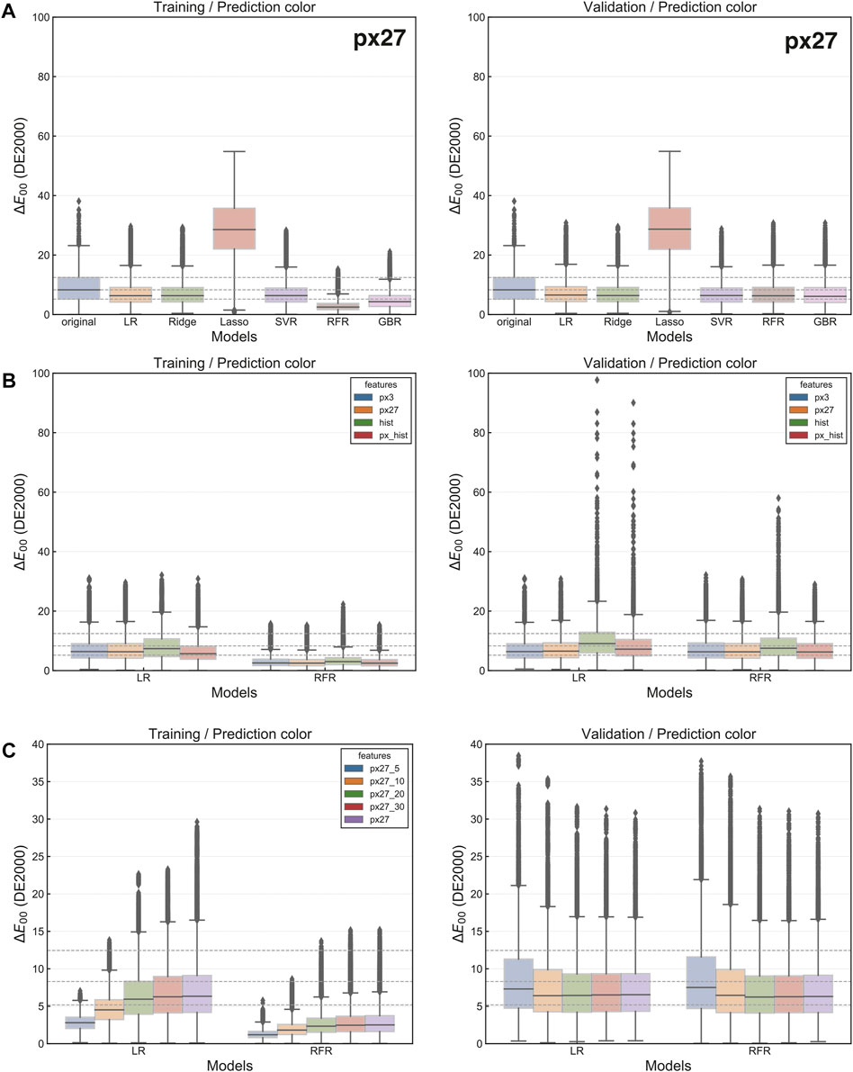
FIGURE 2. Results of model evaluation. All graphs show the difference between the predicted and apparent colors with the DE2000 metric. The left-hand side shows the prediction results for training data, while the right-hand side shows the prediction results for validation data. (A) Prediction performance with various model structures and px27 features. (B) Prediction performance with various features on LR and RFR models. (C) Prediction performance with various ranges of training data.

It should be noted that models and features are not independent, and their performance may vary depending on their combination. Consequently, the applicability of model-selection results employing px27 features (Figure 2A) would not be generalized for alternative features. Nevertheless, the authors’ supplemental experiments indicated no combination that yielded a more substantial improvement in performance than the one presented in Figure 2A. For example, GBR (the pink box in Figure 2A), a decision tree-oriented framework like the RFR model, exhibits comparable performance. Nonetheless, no discrepancies in the validation data outcomes when employing RFR, thereby omitting the detailed results of GBR in the subsequent discussion. Results on combinations absent from Figure 2A are included as the Supplementary Data.

2.2.2.2 Which features are suitable? (Point 2)

The prediction performance of the apparent color with feature configurations is shown in Figure 2B. The graphs for the LR model (the left-half of each graph) confirm that the prediction performance deteriorated significantly when histogram features were used. The deterioration in prediction performance is thought to be due to multicollinearity. However, the RFR model results (the right-half of each graph) show that such deterioration only occurred when the histogram features without pixel values were used. For the features that did not worsen the prediction performance, there was no significant difference in prediction performance between the LR and RFR. Thus, the aspects without histogram features are suitable: px27 (multi-scale, the orange box) or px3 (single-scale, the blue box). For the robustness of the prediction and reflection of the adjacent colors, the px27 features were adopted in this study.

2.2.2.3 What is the appropriate range of training data? (Point 3)

Dataset with pronounced color differences in the apparent color dataset (Kubota et al., 2022) may have been caused by participants’ failure to adjust their apparent color properly. Owing to the potential risk of incorporating such outlier data on prediction accuracy, the authors examined Point 3.

The prediction performance of the apparent color with the range of training data is shown in Figure 2C. The smaller difference on the left side of each graph for the training data is due to the smaller range of the training data. However, the results for the validation data indicate that the prediction performance improved from px27_5 (the blue box) to px27_20 (the green box) and is almost constant for px27_20 and above. There is no deterioration in the prediction performance even when all data is used as the training data. Thus, the authors set no restriction for the data range.

From these evaluations, the authors adopted the LR model as the model structure, px27 features as the feature vectors, and no restrictions for the data range of color difference.

2.2.2.4 How much does the comparator improve the prediction? (Point 4)

Here, the authors investigate the influence of the comparator on the prediction performance. The detailed structure of the comparator was explained in Section 2.2.1.

Histograms of the predicted color with and without the comparator are shown in Figure 3. The horizontal axis denotes the DE2000 color difference between the predicted color and the apparent color: the red line shows the original pixel color, the green line shows the color predicted by the model with the comparator, and the blue line shows the color predicted by the model without the comparator. The color differences obtained over 100 trials (100 different data combinations) for the validation data were ΔE₀₀ = 7.14 ± 0.29 for the model with comparator, ΔE₀₀ = 7.33 ± 0.25 for the model without the comparator, and ΔE₀₀ = 9.54 ± 0.36 for original pixel color. Thus, it is confirmed that the predicted colors were closer to the apparent color than the pixel color, regardless of whether the comparator model was present.

FIGURE 3

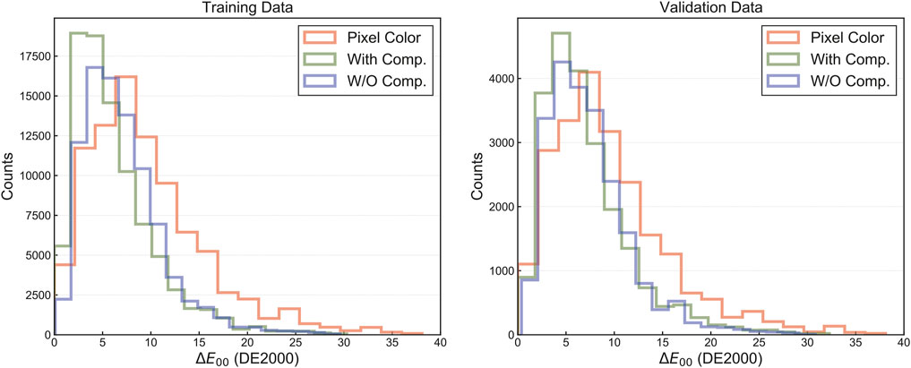
FIGURE 3. Histograms of predicted colors with and without adding a comparator. The horizontal axis denotes the color difference between the predicted or pixel color and the apparent color based on the DE2000 metric; the red line shows the pixel color, the green line shows the predicted color of the model with the comparator, and the blue line shows the predicted color of the model without the comparator.

Furthermore, comparing the improved rate of the predictions from the original pixel color, the model with the comparator had an improved rate of R = 0.770 ± 0.028, and the model without the comparator had an improved rate of R = 0.688 ± 0.029. From this consideration, the model with the comparator was found to have a higher rate of improvement than the model without the comparator. Based on these results, the authors adopted the model with the comparator, and conducted the evaluation experiments described in the following section.

2.3 Stimuli and procedures of evaluation experiments

To verify the performance of the proposed model as an apparent color picker, evaluation experiments were conducted. The authors evaluated the model performance based on the dataset with texture images and the dataset with landscape images. Additionally, the prediction model was compared with the model that only corrected for L* or a*b*.

2.3.1 Stimuli

Candidate stimuli were selected from images in the DTD dataset (Cimpoi et al., 2014) and the Places dataset (Zhou et al., 2017). The DTD dataset is used for constructing the apparent color dataset and consists of photographs, mainly texture images. The Places dataset mainly contains landscape photographs with three-dimensional objects. By recruiting two datasets, the authors evaluated whether the proposed method could be applied to a broader range of images. Note that the images in the Places dataset were scaled down to 75% of their original size. Rescaled images with a size of 640 px or less were selected due to the size limit of the task screen after it was rescaled.

The candidate stimuli were first collected as 10,000 image-position pairs from the DTD dataset and 20,000 image-position pairs from the Places dataset, following the previous paper constructing the apparent color dataset (Kubota et al., 2022). The pairs of image and response position were selected so that the color difference ΔE₀₀ < 5.0 in the range of 5 px surroundings of the position to be responded to. When using a color picker interface, the users are expected to select colors from areas with a certain degree of color uniformity. The Places dataset was found to have a more significant bias in luminance and color distributions than the DTD dataset. Thus, 20,000 candidates were collected for the Places dataset.

The stimuli presented to each participant included 66 pictures from the DTD and Places datasets as described below. Due to the existence of bias in the L*a*b* values of the photographs, the image-position pairs were categorized into nine blocks: three levels of luminance $L^{*}=\left.\left[\mathrm{0,30}\right.\right),\left.\left[\mathrm{30,60}\right.\right),[\mathrm{60,100}]$ and three levels of saturation $a^{*}{b}^{*}=\sqrt{a^{*2}+b^{*2}}=\left.\left[\mathrm{0,30}\right.\right),\left.\left[\mathrm{30,60}\right.\right),[\mathrm{60,144}]$. By selecting images from each block equally, a wide range of data from low saturation (low luminance) to high saturation (high luminance) could be evaluated. However, in both datasets, the pair $L^{*}=\left.\left[\mathrm{0,30}\right.\right)$ and a*b* = [60, 144] (Category [0,2], Category 2) had very few candidate images compared to the other eight categories. Thus, only two images were extracted from this category. As a result, a set of 66 images and response positions, two from the Category [0,2] (Category 2), and eight from the other eight categories, were randomly selected from each category. By changing the images presented to each participant, the authors collected the evaluation for various images.

2.3.2 Procedures

Eleven participants (seven males, four females) aged from 19 to 28 years with normal or corrected vision participated in the experiment. At the beginning of the experiment, a simplified browser-based Ishihara test (Colblindor, 2006) confirmed that all participants had a trichromatic vision. The participants were instructed to observe the display from approximately 60 cm apart, and turn off both night-shift and dark modes on the display. The participants worked on the online experiment created with jsPsych (de Leeuw, 2015) on their PCs. The screen size was scaled using a credit card as a reference of known size. Specifically, the participants adjusted the size of the rectangle on the screen to fit the size of their credit cards. The pre-experimental questionnaire confirmed that most participants rarely (less than once a year) or occasionally (several times a year) work on creative activities related to pictures and colors. In particular, they rarely or occasionally utilized a color picker or a color extraction system.

Figure 4 shows an example of the task screen. The task screen consisted of a stimulus image on the left half and two color squares on the right half. Participants first searched for the area surrounded by a black-and-white border (20 px square, 0.4 cm square) in the stimulus image displayed on the left side. Next, they determined which of the two colored squares in the right half was closer to the apparent color in the area surrounded by the border using the buttons at the bottom of the screen. They were instructed to determine the color near the center of the box where several colors were observed. Although completion of the task had no time limit, median (IQR) of the response time was 4.5 s (3.2 − 6.9 s). Participants were instructed to take 1-min breaks every 20 min. The entire experiment took about 60 min. Before the start of the experiment, four practice stimuli identical to all participants were presented. The practice images were presented in the same order to all participants and were used to check whether the participants performed the experimental task correctly.

FIGURE 4

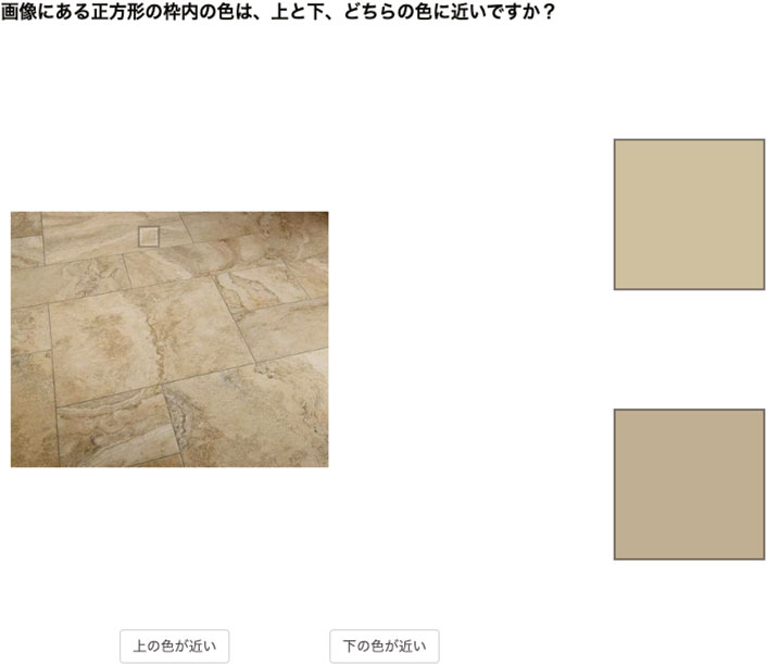
FIGURE 4. Example of the task screen. The left half of the screen displays a stimulus image with a frame indicating the response position. The right half shows two color squares. The participants selected a color from the upper or lower squares closer to the color inside the box. At the top of the task screen, the following question is displayed: “Which color in the square frame in the image is closer to the color of the upper or lower square?”.

In Experiment 1, the prediction performance for the DTD dataset was evaluated; a total of 66 stimuli were selected from the 10,000 candidates of the image in the DTD dataset. In Experiment 2, the prediction performance for the Places dataset was evaluated. In Experiment 3, the authors investigated the role of luminance and saturation in the proposed model; a total of 33 stimuli (one from Category 2 and four each from the other eight categories) were selected from the 10,000 candidates in the DTD dataset. Two types of the predicted color were evaluated: one is characterized by L* as the predicted value and a*b* as the pixel value (L* condition), and the other is characterized by a*b* as the predicted value and L* as the pixel value (a*b* condition). For each candidate stimulus, the pixel color and the predicted color of the model were randomly presented in either the upper or lower square. To eliminate the influences of whether the predicted color is displaced at the upper or lower square, two trials were performed for each stimulus, switching the display position of the square corresponding to the predicted color in these three experiments.

3 Results

First, the authors compared the model’s predictions for each of the stratified categories. Figure 5 shows the results of the improved rate summarized for each category. The improved rate indicates the percentage of trials in each category in which the predicted color is closer to the apparent than the pixel color. A higher improved rate means that the predicted color of the model is better at predicting the apparent color in photos for each category than the original pixel color. The summary statics for each category are described in Table 1. Significance levels were corrected using the Bonferroni correction. Specifically, the nine categories were tested as multiple comparisons with N = 18 because these categories were compared to the chance rate for the different datasets.

FIGURE 5

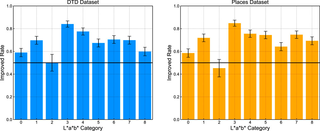
FIGURE 5. Improved rate for each stratified category where categories [0,1,2] denote low luminance, [3,4,5] denote medium luminance, and [6,7,8] denote high luminance. Categories [0,3,6] denote low saturation, [1,4,7] denote medium saturation, and [2,5,8] denote high saturation. Error bars indicate standard errors calculated from a binominal distribution.

TABLE 1

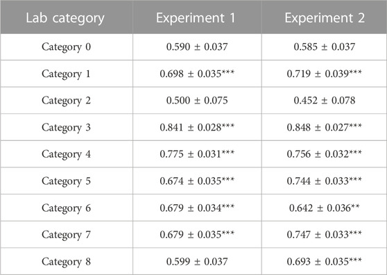
TABLE 1. Summarized statics of improved rate for each category in the stratified extraction. (*: p < 0.05,**: p < 0.01,***:p < 0.001).

The results confirmed an average improvement in the predicted color over the pixel color in most categories. Especially, in Categories 3 and 4 (medium-luminance and low to medium saturation), the improved rate reached 75%–85% for both DTD and Places dataset, suggesting that the proposed model works as an effective prediction tool in this color domain. However, no significant differences were observed for Categories 0 and 2 (low luminance and low or high saturation). Similarly, the performance of Category 8 (high luminance and high saturation) also decreased in the DTD dataset. These results suggest that the model effectively improved the prediction accuracy in the mid-luminance region by more than 70%. In contrast, the prediction accuracy decreased in low-luminance and high-luminance/high-saturation regions.

Next, the prediction performance according to the color difference between the pixel color and the predicted color was evaluated. A graph summarizing the improved rate for each color difference with the DE2000 metric is shown in Figure 6. The color differences were converted to integer values by the floor function to draw the graph. Note that color differences below 1.0 and above 10.0 had small items (2 − 36 items) in both datasets. Additionally, it should be noted that participants did not directly answer the apparent color in the authors’ evaluation experiments. Figure 6 illustrates the difference between the predicted color and pixel color, not between the apparent color and pixel color. The graph indicates that the improved rate is approximately 70%–80% in the region of the color difference 3.0 < ΔE₀₀ < 10.0. These results suggest that, on average, the model can predict color closer to the apparent color than the pixel color. However, the prediction accuracy decreased in the region of 0.0 ≤ ΔE₀₀ ≤ 3.0. This decrease may be because the participants had difficulty perceiving the difference between the predicted color and the pixel color, i.e., the difficulty in distinguishing between the colors in the upper and lower squares.

FIGURE 6

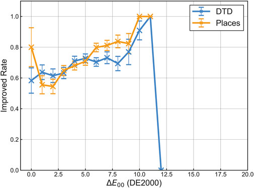
FIGURE 6. Improved rate with the color difference between the pixel color and the predicted color. The color difference of images is measured by the DE2000 metric and classified as an integer value using the floor function. Error bars indicate standard errors calculated from a binominal distribution.

Finally, the improved rate when correcting only for luminance or saturation is summarized. Figure 7 illustrates the prediction results using only luminance (L*) and saturation (a*b*) information. A Student’s t-test considering the Bonferroni correction (N = 3) shows no significant difference between the L*a*b* and L* conditions (p = 0.209). In contrast, there are significant differences between the L*a*b* and a*b* conditions (p < 0.001) and the L* and a*b* conditions (p < 0.001). Thus, in the configuration of this model, information on luminance (L*) could improve prediction accuracy. In contrast, information on saturation (a*b*) had a limited contribution to the prediction improvement.

FIGURE 7

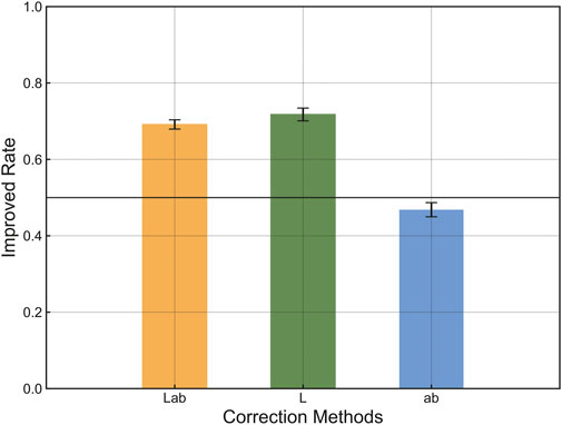
FIGURE 7. Prediction results using only luminance (L*) and saturation (a*b*) information. Error bars indicate standard errors calculated from a binominal distribution.

4 Discussion

The evaluation experiments suggest that the proposed model could predict colors closer to the apparent color than the original pixel color. The luminance correction was particularly adequate for the prediction, as shown in Figure 7. This result can be explained as a result of the influence of the extraction interface in the experiment. The extraction interface displayed the color of a specific part of the photos in a square on a white background. The color shift caused by the simultaneous contrast effect resulted in the square colors on the white background being darker than the original pixel color. To compensate for the simultaneous contrast effects, it is necessary to display brighter colors than the original pixel color. However, the saturation did not contribute to the color prediction. The employed model was a simple linear regression model, which may have effectively corrected for systematic shifts.

However, Figure 5 illustrates that performance deteriorated within specific categories. Notably, performance was limited in the low-luminance region (Categories 0–2) and the high-luminance/high-saturation region (Category 8) compared to the medium-luminance region (Categories 3 and 4). For Category 2, the performance decline stemmed from the minimal number of data. As the probability of extracting this region from natural images is minimal, the authors believe that practical issues for this area would be negligible. Although the authors do not know a conclusive answer for the performance deterioration in the remaining categories, there would be two potential explanations. Firstly, color differences might vary between categories. Analyzing the apparent color dataset (Kubota et al., 2022), the median color differences between the apparent color and pixel color for Categories 0 and 2 were 6.89 and 6.03. Conversely, for Categories 3 and 4, which exhibited superior prediction accuracy, these values increased to 12.7 and 11.8. These results imply that the improvement rate would escalate when the deviation between the original pixel color and the apparent color is more pronounced. Secondly, Figure 7 demonstrates that the proposed system’s saturation correction enhancement is restricted. In the high-saturation region, the prediction accuracy may have diminished due to the inability to represent saturation by the regression model, resulting in a decreased improvement rate. These issues could be resolved by augmenting datasets within these domains and re-selecting more appropriate features and the prediction model.

Moreover, Figure 6 reveals that the performance also degraded in the region where the difference between the original pixel color and the predicted color is minor. During the authors’ assessment, participants were presented with the pixel color and the predicted color and instructed to compare which color was closer to their perception. In areas where color differences are minimal in Figure 6, participants would struggle to distinguish between colors. To take an extreme case, if no color difference existed between the two, the correct response rate would reach approximately 50%. Thus, it would be reasonable for the results to approximate 50% (the proportion of correct answers in the event of random selection) in regions characterized by minimal color differences. In other words, the diminished prediction performance in the realm of minor color discrepancies would constitute an issue inherent to the evaluation experiment design, which might not solve the problem with system improvement.

Below, the authors discuss the influences of the model structure and features on the predictions. The proposed model adopted the multi-scale pixel values (px27) as features. However, the results in Figure 2B suggest that there is no significant difference in the prediction accuracy between the model with single-scale pixel values (px3) and multi-scale pixel values (px27). The results suggest that the improvement in prediction due to considering multi-scale colors was limited. However, it is known that color perception is affected by complex combinations of various factors, such as color constancy, color temperature, higher-order object recognition, and display chromaticity. Features that reflect color temperature and object labels may improve the prediction accuracy of the apparent color.

The authors constructed the color prediction model using a data-driven and linear regression model (Figure 1). Linear models resist over-fitting and allow for reasonable predictions even when the number of data is small. However, a deep learning model, including a convolutional neural network or a biological model referring to the sensory information processing of the brain, would be effective for building color prediction models. When adopting a deep learning model, it would be necessary to design appropriate features or collect additional training data to prevent over-fitting. A biological model based on the brain’s information processing would also be a candidate for the apparent color picker. Although no unified color perception model has been proposed, computational models that reflect color perception characteristics were reported (Moroney et al., 2002). As human color perception involves environmental and physical factors, including lighting environment and illumination, it would be necessary to calibrate such models to environmental conditions.

The apparent color picker may be affected by the characteristics and arrangement of the user interface. The experimental participants used an interface with a white background because participants were asked to turn off the night-shift and dark modes of the browser during the experiment. Given the property of the simultaneous contrast effect, the direction of the luminance shift is expected to be nearly reversed. Constructing a prediction model compatible with dark mode may be possible by reversing the direction of the luminance shift. Although the scale of the displayed image would affect the predictions, the proposed model could cope with changes in image size by constructing multi-scale features that correspond to the image size.

However, the inability to reproduce parts of the apparent color when the model extracts the apparent color from photographs to the square on a white background is a significant limitation. Owing to the different surrounding colors, the representable range of colors would differ between the photos and the square on the white background. The methodology to overcome this limitation requires hardware-based improvement of the display. This issue would not be solved by software-based improvements, such as the construction of color prediction models.

By combining the color extraction model of this paper and its reversed model, it may be possible to construct a color transfer model that reproduces the colors from one image to another. To achieve this, it may be necessary to include object recognition techniques related to both lower-order relationships with surrounding colors and the context of images for higher-order cognition. This color transfer model may be utilized to transform not only the pixel-wise color itself but the surrounding color so that the color context of the images preserves.

Dealing with human perception and cognition, physical measurements are often taken as the correct values, and human perception is often described as inaccurate or biased. The manifested discrepancies between these two states are often called illusions. However, the world recognized by humans and computers cannot have one being correct and the other wrong. Illusions are caused by the sensory information processing of the brain, which is influenced by various factors, including physical objects, brain functions, environment, knowledge, and memories. Properly measuring the gaps between the “perceptual” world of humans and computers and building a model that grasps human perception based on the gaps are essential in dealing with illusions. By constructing the apparent color prediction model, this study has reached a milestone in capturing the characteristics of human perception in a daily environment.

5 Conclusion

In this paper, the authors investigated the suitable model structure and features for an apparent color picker that extracts the apparent color from photographs. First, the regression model was constructed to predict the apparent color using the apparent color dataset collected by psychophysical experiments, which is annotated with the apparent color that participants perceived in photos. Based on the performance evaluation for various models and features, a linear regression model with features that reflect the adjacent color in multi-scale (px27 features) was suitable for predicting the apparent color. A comparator was built into the prediction model to prevent deteriorating the accuracy when there was a slight difference between the predicted and pixel colors. To assess the performance in the actual situations, evaluation experiments were conducted with the inclusion of eleven participants. These evaluations utilized images extracted from two different datasets: the DTD dataset and the Places dataset. The results indicated that the estimated color was closer to the apparent color than the pixel color for 75%–85% of trials at medium luminance and low or medium saturation. However, the improved rate decreased in accuracy under several conditions with low luminance images. In conclusion, evaluation experiments confirmed that the proposed model could predict the apparent color to some extent. In contrast, it is suggested that further improvement could be achieved by taking into account factors that the model did not incorporate, such as the influences of higher-order cognition and illuminant information.

Data availability statement

The datasets presented in this study can be found in online repositories. The names of the repository/repositories and accession number(s) can be found below: https://drive.google.com/drive/folders/1Z7m2OWB1BP1p375NUW8YUi9UyJMFxLP9?usp&equals;share_link.

Ethics statement

The studies involving human participants were reviewed and approved by the Institutional Review Board at the University of Tokyo. For the online experiments, the participants provided their electronic informed consent to participate in this study.

Author contributions

YK designed and supervised the study, conducted experiments, collected data, validated the results, drafted, reviewed, and revised the manuscript. SY reviewed the experimental methodology, reviewed, and revised the manuscript. MI supervised the study and proofread the manuscript. All authors have read and agreed to the published version of the manuscript.

Funding

This research was financially supported by the funding of JST ERATO Grant Number JPMJER1701 and JST Moonshot R&D Program Grant Number JPMJMS2292, Japan.

Acknowledgments

The authors are grateful to Sohei Wakisaka (the University of Tokyo, Japan), Rira Miyata (the University of Tokyo, Japan), and Yuki Koyama (National Institute of Advanced Industrial Science and Technology, Japan) for helpful discussions.

Conflict of interest

The authors declare that the research was conducted in the absence of any commercial or financial relationships that could be construed as a potential conflict of interest.

Publisher’s note

All claims expressed in this article are solely those of the authors and do not necessarily represent those of their affiliated organizations, or those of the publisher, the editors and the reviewers. Any product that may be evaluated in this article, or claim that may be made by its manufacturer, is not guaranteed or endorsed by the publisher.

Supplementary material

The Supplementary Material for this article can be found online at: https://www.frontiersin.org/articles/10.3389/frsip.2023.1133210/full#supplementary-material

References

Agarwal, V., Gribok, A. V., and Abidi, M. A. (2007). Machine learning approach to color constancy. Neural Netw. 20, 559–563. doi:10.1016/j.neunet.2007.02.004

PubMed Abstract | CrossRef Full Text | Google Scholar

Akazawa, T., Kinoshita, Y., Shiota, S., and Kiya, H. (2022). N-white balancing: White balancing for multiple illuminants including non-uniform illumination. IEEE Access 10, 89051–89062. doi:10.1109/access.2022.3200391

CrossRef Full Text | Google Scholar

Akbarinia, A., and Parraga, C. A. (2017). Colour constancy beyond the classical receptive field. IEEE Trans. pattern analysis Mach. Intell. 40, 2081–2094. doi:10.1109/tpami.2017.2753239

PubMed Abstract | CrossRef Full Text | Google Scholar

Anderson, B. L. (1997). A theory of illusory lightness and transparency in monocular and binocular images: The role of contour junctions. Perception 26, 419–453. doi:10.1068/p260419

PubMed Abstract | CrossRef Full Text | Google Scholar

Anderson, M., Motta, R., Chandrasekar, S., and Stokes, M. (1996). “Proposal for a standard default color space for the internet—sRGB,” in Proceedings of Color and Imaging Conference (Scottsdale, Arizona, United States: Society for Imaging Science and Technology (IS&T)), 238–245.

Google Scholar

Bailey, P., Manktelow, K., and Olomolaiye, P. (2003). “Examination of the color selection process within digital design for the built environment,” in Proceedings of theory and practice of computer graphics, 2003 (Birmingham, United Kingdom: IEEE (Institute of Electrical and Electronics Engineers)), 193–200.

Google Scholar

Barron, J. T. (2015). “Convolutional color constancy,” in Proceedings of the IEEE international conference on computer vision (Santiago, Chile: IEEE), 379–387.

CrossRef Full Text | Google Scholar

Bergman, L. D., Rogowitz, B. E., and Treinish, L. A. (1995). “A rule-based tool for assisting colormap selection,” in Proceedings of visualization 1995 (Atlanta, Georgia, United States: IEEE), 118–125.

Google Scholar

Bertalmío, M., Caselles, V., Provenzi, E., and Rizzi, A. (2007). Perceptual color correction through variational techniques. IEEE Trans. Image Process. 16, 1058–1072. doi:10.1109/tip.2007.891777

PubMed Abstract | CrossRef Full Text | Google Scholar

Boynton, R. M., and Purl, K. (1989). Categorical colour perception under low-pressure sodium lighting with small amounts of added incandescent illumination. Light. Res. Technol. 21, 23–27. doi:10.1177/096032718902100104

CrossRef Full Text | Google Scholar

Cheng, D., Prasad, D. K., and Brown, M. S. (2014). Illuminant estimation for color constancy: Why spatial-domain methods work and the role of the color distribution. JOSA A 31, 1049–1058. doi:10.1364/josaa.31.001049

PubMed Abstract | CrossRef Full Text | Google Scholar

Cimpoi, M., Maji, S., Kokkinos, I., Mohamed, S., and Vedaldi, A. (2014). “Describing textures in the wild,” in Proceedings of the IEEE conference on computer vision and pattern recognition (Columbus, Ohio, United States: IEEE), 3606–3613.

CrossRef Full Text | Google Scholar

Cohen-Or, D., Sorkine, O., Gal, R., Leyvand, T., and Xu, Y.-Q. (2006). “Color harmonization,” in ACM SIGGRAPH 2006 papers (ACM) (Boston, Massachusetts, United States: ACM (Association for Computing Machinery)), 624–630.

CrossRef Full Text | Google Scholar

Colblindor (2006). Ishihara 38 plates CVD test. Available at: https://www.color-blindness.com/ishihara-38-plates-cvd-test/.

Google Scholar

de Leeuw, J. R. (2015). jsPsych: A javascript library for creating behavioral experiments in a web browser. Behav. Res. methods 47, 1–12. doi:10.3758/s13428-014-0458-y

PubMed Abstract | CrossRef Full Text | Google Scholar

Dixon, E. L., and Shapiro, A. G. (2017). Spatial filtering, color constancy, and the color-changing dress. J. Vis. 17, 7. doi:10.1167/17.3.7

PubMed Abstract | CrossRef Full Text | Google Scholar

Douglas, S. A., and Kirkpatrick, A. E. (1999). Model and representation: The effect of visual feedback on human performance in a color picker interface. ACM Trans. Graph. (TOG) 18, 96–127. doi:10.1145/318009.318011

CrossRef Full Text | Google Scholar

Ebbinason, A. G., and Kanna, B. R. (2014). “ColorFingers: Improved multi-touch color picker,” in SIGGRAPH asia 2014 technical briefs (ACM) (Shenzhen, China: ACM), 1–4.

Google Scholar

Ebner, M. (2012). A computational model for color perception. Bio-Algorithms and Medical-Systems 8 (4), 387–415.

CrossRef Full Text | Google Scholar

Finlayson, G. D., and Hordley, S. D. (2001). Color constancy at a pixel. J. Opt. Soc. Am. A 18, 253–264. doi:10.1364/josaa.18.000253

PubMed Abstract | CrossRef Full Text | Google Scholar

Gijsenij, A., Gevers, T., and van de Weijer, J. (2011). Computational color constancy: Survey and experiments. IEEE Trans. image Process. 20, 2475–2489. doi:10.1109/tip.2011.2118224

PubMed Abstract | CrossRef Full Text | Google Scholar

Gomez-Villa, A., Martín, A., Vazquez-Corral, J., Bertalmío, M., and Malo, J. (2020). Color illusions also deceive CNNs for low-level vision tasks: Analysis and implications. Vis. Res. 176, 156–174. doi:10.1016/j.visres.2020.07.010

PubMed Abstract | CrossRef Full Text | Google Scholar

Granzier, J. J., Brenner, E., and Smeets, J. B. (2009). Do people match surface reflectance fundamentally differently than they match emitted light? Vis. Res. 49, 702–707. doi:10.1016/j.visres.2009.01.004

PubMed Abstract | CrossRef Full Text | Google Scholar

Granzier, J. J., and Gegenfurtner, K. R. (2012). Effects of memory colour on colour constancy for unknown coloured objects. i-Perception 3, 190–215. doi:10.1068/i0461

PubMed Abstract | CrossRef Full Text | Google Scholar

Harrower, M., and Brewer, C. A. (2003). Colorbrewer.org: An online tool for selecting colour schemes for maps. Cartogr. J. 40, 27–37. doi:10.1179/000870403235002042

CrossRef Full Text | Google Scholar

Hedrich, M., Bloj, M., and Ruppertsberg, A. I. (2009). Color constancy improves for real 3D objects. J. Vis. 9, 16. doi:10.1167/9.4.16

PubMed Abstract | CrossRef Full Text | Google Scholar

Hirsch, E., and Tal, A. (2020). “Color visual illusions: A statistics-based computational model,” in 34th conference on neural information processing systems (NeurIPS 2020), 9447–9458.

Google Scholar

Hussain, M. A., Sheikh-Akbari, A., and Halpin, E. A. (2019). Color constancy for uniform and non-uniform illuminant using image texture. IEEE Access 7, 72964–72978. doi:10.1109/access.2019.2919997

CrossRef Full Text | Google Scholar

Jain, J., Bhatti, N., Baker, H., Chao, H., Dekhil, M., Harville, M., et al. (2008). “Color match: An imaging based mobile cosmetics advisory service,” in Proceedings of the 10th international conference on Human computer interaction with mobile devices and services, 331–334.

Google Scholar

Johnson, G. M., and Fairchild, M. D. (2003). A top down description of S-CIELAB and CIEDE2000. Color Res. Appl., 28, 425–435.

CrossRef Full Text | Google Scholar

Kim, M. H., Weyrich, T., and Kautz, J. (2009). Modeling human color perception under extended luminance levels. ACM Trans. Graph. 28, 1–9. doi:10.1145/1531326.1531333

CrossRef Full Text | Google Scholar

Klauke, S., and Wachtler, T. (2015). Tilt” in color space: Hue changes induced by chromatic surrounds. J. Vis. 15, 17. doi:10.1167/15.13.17

PubMed Abstract | CrossRef Full Text | Google Scholar

Kubota, Y., Hiyama, A., and Inami, M. (2021). “A machine learning model perceiving brightness optical illusions: Quantitative evaluation with psychophysical data,” in Proceedings of augmented humans conference 2021 (ACM), 174–182.

CrossRef Full Text | Google Scholar

Kubota, Y., Yoshida, S., and Inami, M. (2022). “Apparent color dataset: How apparent color differs from the color extracted from photos,” in Proceedings on IEEE international conference on systems, man, and cybernetics (SMC) 2022 (Prague, Czech Republic: IEEE), 261–267.

CrossRef Full Text | Google Scholar

Kuriki, I. (2018). A novel method of color appearance simulation using achromatic point locus with lightness dependence. i-Perception 9, 204166951876173. doi:10.1177/2041669518761731

PubMed Abstract | CrossRef Full Text | Google Scholar

Kuriki, I. (2015). Effect of material perception on mode of color appearance. J. Vis. 15, 4. doi:10.1167/15.8.4

PubMed Abstract | CrossRef Full Text | Google Scholar

Kuriki, I., and Uchikawa, K. (1996). Limitations of surface-color and apparent-color constancy. J. Opt. Soc. Am. A 13, 1622–1636. doi:10.1364/josaa.13.001622

PubMed Abstract | CrossRef Full Text | Google Scholar

Lafer-Sousa, R., and Conway, B. R. (2017). #TheDress: Categorical perception of an ambiguous color image. J. Vis. 17, 25. doi:10.1167/17.12.25

PubMed Abstract | CrossRef Full Text | Google Scholar

Luo, M. R., and Pointer, M. (2018). CIE colour appearance models: A current perspective. Light. Res. Technol. 50, 129–140. doi:10.1177/1477153517722053

CrossRef Full Text | Google Scholar

MacEachren, A. M., Hardisty, F., Gahegan, M., Wheeler, M., Dai, X., Guo, D., et al. (2001). “Supporting visual integration and analysis of geospatially-referenced data through web-deployable, cross-platform tools,” in Proceedings of national conference for digital government research (citeseer) (Los Angeles, California, United States: ACM), 17–24.

Google Scholar

Meier, B. J., Spalter, A. M., and Karelitz, D. B. (2004). Interactive color palette tools. IEEE Comput. Graph. Appl. 24, 64–72. doi:10.1109/mcg.2004.1297012

PubMed Abstract | CrossRef Full Text | Google Scholar

Moroney, N., Fairchild, M. D., Hunt, R. W., Li, C., Luo, M. R., and Newman, T. (2002). “The CIECAM02 color appearance model,” in Proceedings of color and imaging conference (Scottsdale, Arizona, United States: Society for Imaging Science and Technology (IS&T)), 23–27.

Google Scholar

Okabe, M., Matsushita, Y., Shen, L., and Igarashi, T. (2007). “Illumination brush: Interactive design of all-frequency lighting,” in Proceedings of 15th pacific conference on computer graphics and applications (Maui, Hawaii, United States: IEEE), 171–180.

CrossRef Full Text | Google Scholar

Qian, Y., Chen, K., Nikkanen, J., Kamarainen, J.-K., and Matas, J. (2017). “Recurrent color constancy,” in Proceedings of the IEEE international conference on computer vision (Venice, Italy: IEEE), 5458–5466.

CrossRef Full Text | Google Scholar

Reinhard, E., Adhikhmin, M., Gooch, B., and Shirley, P. (2001). Color transfer between images. IEEE Comput. Graph. Appl. 21, 34–41. doi:10.1109/38.946629

CrossRef Full Text | Google Scholar

Robertson, A. R. (1977). The cie 1976 color-difference formulae. Color Res. Appl. 2, 7–11. doi:10.1002/j.1520-6378.1977.tb00104.x

CrossRef Full Text | Google Scholar

Ryokai, K., Marti, S., and Ishii, H. (2004). “I/O brush: Drawing with everyday objects as ink,” in Proceedings of the 2004 CHI conference on human factors in computing systems (Vienna, Austria: ACM), 303–310.

Google Scholar

Sandnes, F. E., and Zhao, A. (2015). An interactive color picker that ensures WCAG2. 0 compliant color contrast levels. Procedia Comput. Sci. 67, 87–94. doi:10.1016/j.procs.2015.09.252

CrossRef Full Text | Google Scholar

Shapiro, A., Hedjar, L., Dixon, E., and Kitaoka, A. (2018). Kitaoka’s tomato: Two simple explanations based on information in the stimulus. i-Perception 9, 204166951774960. doi:10.1177/2041669517749601

CrossRef Full Text | Google Scholar

Shapiro, A., and Lu, Z.-L. (2011). Relative brightness in natural images can be accounted for by removing blurry content. Psychol. Sci. 22, 1452–1459. doi:10.1177/0956797611417453

PubMed Abstract | CrossRef Full Text | Google Scholar

Sharma, G., Wu, W., and Dalal, E. N. (2005). The CIEDE2000 color-difference formula: Implementation notes, supplementary test data, and mathematical observations. Color Res. Appl. 30, 21–30. doi:10.1002/col.20070

CrossRef Full Text | Google Scholar

Shugrina, M., Lu, J., and Diverdi, S. (2017). Playful palette: An interactive parametric color mixer for artists. ACM Trans. Graph. (TOG) 36, 1–10. doi:10.1145/3072959.3073690

CrossRef Full Text | Google Scholar

Shugrina, M., Zhang, W., Chevalier, F., Fidler, S., and Singh, K. (2019). “Color builder: A direct manipulation interface for versatile color theme authoring,” in Proceedings of the 2019 CHI conference on human factors in computing systems (Glasgow, Scotland, United Kingdom: ACM), 1–12.

Google Scholar

Sidorov, O. (2019). “Conditional GANs for multi-illuminant color constancy: Revolution or yet another approach?,” in Proceedings of the IEEE/CVF conference on computer vision and pattern recognition workshops (Long Beach, California, United States: IEEE), 1748–1758.

CrossRef Full Text | Google Scholar

Solmaz, M. E., Mutlu, A. Y., Alankus, G., Kılıç, V., Bayram, A., and Horzum, N. (2018). Quantifying colorimetric tests using a smartphone app based on machine learning classifiers. Sensors Actuators B Chem. 255, 1967–1973. doi:10.1016/j.snb.2017.08.220

CrossRef Full Text | Google Scholar

Vršnak, D., Domislović, I., Subašić, M., and Lončarić, S. (2023). Framework for illumination estimation and segmentation in multi-illuminant scenes. IEEE Access 11, 2128–2137. doi:10.1109/access.2023.3234115

CrossRef Full Text | Google Scholar

Wang, Y., Zhang, J., Cao, Y., and Wang, Z. (2017). “A deep CNN method for underwater image enhancement,” in 2017 IEEE international conference on image processing (ICIP) (Beijing, China: IEEE), 1382–1386.

CrossRef Full Text | Google Scholar

Wijffelaars, M., Vliegen, R., van Wijk, J. J., and van der Linden, E.-J. (2008). Generating color palettes using intuitive parameters. Comput. Graph. Forum 27, 743–750. doi:10.1111/j.1467-8659.2008.01203.x

CrossRef Full Text | Google Scholar

Wong, B. (2010). Points of view: Color coding. Nat. Methods 7, 573. doi:10.1038/nmeth0810-573

PubMed Abstract | CrossRef Full Text | Google Scholar

Wu, Y., and Takatsuka, M. (2005). “Three dimensional colour pickers,” in Proceedings of the 2005 asia-pacific symposium on information visualization (Sydney, Australia: Australian Computer Society), 107–114.

Google Scholar

Yuan, L., Zhou, Z., Zhao, J., Guo, Y., Du, F., and Qu, H. (2021). InfoColorizer: Interactive recommendation of color palettes for infographics. IEEE Trans. Vis. Comput. Graph. 28, 4252–4266. doi:10.1109/tvcg.2021.3085327

CrossRef Full Text | Google Scholar

Zhai, Q., and Luo, M. R. (2018). Study of chromatic adaptation via neutral white matches on different viewing media. Opt. express 26, 7724–7739. doi:10.1364/oe.26.007724

PubMed Abstract | CrossRef Full Text | Google Scholar

Zhang, M., Qiu, G., Alechina, N., and Atkinson, S. (2013). “User study on color 1459 palettes for drawing query on touchscreen phone,” in Proceedings of the 2nd International Conference on Human-Computer Interaction, Prague, Czech Republic, August 14–15, 2014, 134.

Google Scholar

Zhou, B., Lapedriza, A., Khosla, A., Oliva, A., and Torralba, A. (2017). Places: A 10 million image database for scene recognition. IEEE Trans. pattern analysis Mach. Intell. 40, 1452–1464. doi:10.1109/tpami.2017.2723009

PubMed Abstract | CrossRef Full Text | Google Scholar

Zini, S., Buzzelli, M., Bianco, S., and Schettini, R. (2022). Cocoa: Combining color constancy algorithms for images and videos. IEEE Trans. Comput. Imaging 8, 795–807. doi:10.1109/tci.2022.3203889

CrossRef Full Text | Google Scholar