 Marco Comunità
 Christian J. Steinmetz
 Joshua D. Reiss
- Centre for Digital Music, School of Electronic Engineering and Computer Science, Queen Mary University of London, London, United Kingdom
Audio effects are extensively used at every stage of audio and music content creation. The majority of differentiable audio effects modeling approaches fall into the black-box or gray-box paradigms; and most models have been proposed and applied to nonlinear effects like guitar amplifiers, overdrive, distortion, fuzz and compressor. Although a plethora of architectures have been introduced for the task at hand there is still lack of understanding on the state of the art, since most publications experiment with one type of nonlinear audio effect and a very small number of devices. In this work we aim to shed light on the audio effects modeling landscape by comparing black-box and gray-box architectures on a large number of nonlinear audio effects, identifying the most suitable for a wide range of devices. In the process, we also: introduce time-varying gray-box models and propose models for compressor, distortion and fuzz, publish a large dataset for audio effects research—ToneTwist AFx—that is also the first open to community contributions, evaluate models on a variety of metrics and conduct extensive subjective evaluation. Code and supplementary material are also available.
1 Introduction
Audio effects are central for engineers and musicians to shape the timbre, dynamics, and spatialisation of sound (Wilmering et al., 2020). For some instruments (e.g., electric guitar) the processing chain is part of the artist’s creative expression (Case, 2010) and music genres and styles are also defined by the type of effects adopted (Blair, 2015; Williams, 2012); with renowned musicians adopting specific combinations to achieve a unique sound (Prown and Sharken, 2003). Therefore, research related to audio effects, especially with the success of deep learning (Bengio et al., 2017) and differentiable digital signal processing (DDSP) (Engel et al., 2020), is a very active field (Comunita and Reiss, 2024), with many avenues of investigation open, like: audio effects classification and identification (Comunità et al., 2021; Hinrichs et al., 2022), settings or coefficients estimation and extraction (Kuznetsov et al., 2020; Nercessian, 2020; Colonel et al., 2022b), modeling (Martínez Ramírez, 2021; Wright et al., 2023), processing graph estimation (Lee et al., 2023, 2024) and style transfer (Steinmetz et al., 2022; Vanka et al., 2024; Steinmetz et al., 2024), automatic mixing (Steinmetz et al., 2021; Martínez-Ramírez et al., 2022) or reverse engineering of a mix (Colonel et al., 2022a; Colonel and Reiss, 2023).1,2,3
One of the most active, driven by interest in emulating vintage or costly analog devices, is audio effects modeling (virtual analog), often categorized into white-, gray-, and black-box approaches (see Section 2); and, when using techniques that support gradient backpropagation, referred to as differentiable white-, gray- and black-box. Differentiable methods, leveraging data for gradient descent, are widely used to learn audio effect models. Efforts focus on developing architectures that are both accurate and computationally efficient while being expressive enough to model diverse effect categories and devices 1–3.
Of the three macro categories of audio effects - linear (e.g., EQ, reverb), nonlinear (e.g., distortion, compression), and modulation (e.g., phaser, flanger) - nonlinear effects have received the most attention, with architectures mainly proposed for black- and gray-box methods (see Secs. 2.7, 2.8). Most nonlinear audio effects models focus on a single category (e.g., guitar amplifiers, distortion, compressors) and are evaluated on a single or limited set of devices. Despite the effort, there is no clear state of the art yet that identifies the best-performing approach, particularly for developing architectures that can reliably model all types of nonlinear effects across a wide range of devices. Also, all previous works train and evaluate on data recorded from the same sources (e.g., a specific electric guitar or bass) and very similar content, playing techniques and style, not allowing to reach a reliable conclusion about the generalization capabilities of a trained model. In most cases, training and testing data is normalized without verifying the input dynamic range, not ensuring trained models to be accurate across signal levels.
Therefore, to overcome these limitations, assess the state of the art, and identify research directions, we conduct extensive experiments. In doing so, our work contributes mainly in the following ways:
The remainder of the paper is organized as follows. In Section 2, we outline non-differentiable and differentiable white-, gray-, and black-box approaches to audio effects modeling. Sections 3.1, 3.2 describe the black- and gray-box architectures included in our experiments, while the ToneTwist AFx dataset is described in 3.3. Experiments and results are illustrated and discussed in Sections 4, 5, and objective and subjective evaluations are presented in Section 6. We conclude the manuscript in Section 7.
2 Background
2.1 Nonlinear audio effects modeling
The first thorough investigation of nonlinear distortion for musical applications is (Le Brun’s 1979 work on waveshaping (Le Brun, 1979) and Roads’ subsequent tutorial (Roads, 1979). In the following decades, numerous techniques were developed to digitally simulate or emulate nonlinear analog circuits and devices. This is why we now have approaches based on: solving or approximating the equations describing a system’s behavior, wave digital filters, state-space modeling, Volterra series or Wiener-Hammerstein models, just to name a few. And, with the advancement of machine learning, neural networks based modeling and differentiable DSP have been added to the state of the art.
Audio effects modeling approaches can be categorized into white-, gray-, and black-box, based on the degree of prior knowledge applied, and further classified as differentiable if they support gradient backpropagation. The following sections review previous work on nonlinear audio effects modeling and describe emulation paradigms and techniques.
2.2 White-box modeling
White-box modeling relies on full system knowledge, using differential equations to describe its behavior and numerical methods to solve them in the continuous or discrete domain. These models provide accurate results, making them ideal for replicating specific analog devices. Although, they can be time-consuming to develop, require exact knowledge of the equations describing nonlinear elements and access to the circuit schematic, do not generalize to different devices, and can result in substantial computational load.
Simple systems can be modeled manually by solving the equations (Yeh et al., 2007a; D’Angelo and Välimäki, 2014; Esqueda et al., 2017a); but, for more complex cases, there exist general-purpose frameworks like: state-space models (Mačák, 2012; Holters and Zölzer, 2015; Yeh et al., 2009), wave digital filters (Werner et al., 2015c; De Sanctis and Sarti, 2009; D’Angelo et al., 2012), port-hamiltonian systems (Falaize and Hélie, 2016).
In practice, solving equations have mostly been applied to a small subset of single nonlinear processing blocks like: vacuum tube (Sapp et al., 1999; Karjalainen et al., 2006; Dempwolf and Zölzer, 2011) or transistor stages (D’Angelo et al., 2019), diode clippers (Yeh et al., 2007a; Germain and Werner, 2015; D’Angelo et al., 2019), transformers (Macak, 2011), moog ladder filter (D’Angelo and Välimäki, 2013; D’Angelo and Välimäki, 2014) or the Buchla 259 wavefolder (Esqueda et al., 2017b). But there are also examples of literature modeling complete devices with this method (Yeh et al., 2007b; Macak, 2013).
The most studied white-box modeling framework is wave digital filters (WDF), which emulates analog circuits using traveling wave (scattering) theory and wave variables (instead of voltages and currents), preserving properties like passivity and energy conservation for stable, robust digital implementation.4 (Fettweis, 1986).
Beside single nonlinear blocks like: vacuum tube (Karjalainen and Pakarinen, 2006; Yeh and Smith, 2008; D’Angelo and Välimäki, 2012) or transistor stages (Yeh and Smith, 2008; Yeh, 2009; Bogason, 2018), diode clippers (Yeh et al., 2008; Yeh and Smith, 2008; Werner et al., 2015a; Bernardini and Sarti, 2017), opamps (Yeh, 2009; Bogason and Werner, 2017), nonlinear filters (Werner et al., 2015b; Bogason, 2018) and transformers (Pakarinen et al., 2009); we also find examples of WDFs applied to complete devices like: overdrive and distortion pedals (Yeh, 2009; Bernardini et al., 2020), amplifiers (Pakarinen et al., 2009; De Sanctis and Sarti, 2009), limiters (Raffensperger, 2012).
Similar observations are valid for state-space methods, which represent an electronic circuit as a system of first-order differential equations, describing the circuit in terms of state variables, inputs, and outputs. Using matrix algebra to model components relationships, this method enables efficient digital simulation of complex analog systems. Methods developed for the simulation of state-space systems include the K-method (Yeh and Smith, 2006; Yeh, 2009) the Nodal K-method (or NK-method) and the Discrete K-method (or DK-method or Nodal DK-method) (Yeh, 2009; Yeh et al., 2009).
Examples of state-space methods applied to single nonlinear blocks include: vacuum tubes, transistors, diode clippers and opamps (Yeh and Smith, 2008; Yeh, 2009; Yeh et al., 2009), or transformers (Holters and Zölzer, 2016). But also find examples of emulation of complete devices like: overdrive and distortion (Yeh, 2009; Holmes and van Walstijn, 2015), fuzz (Holmes et al., 2017; Bennett, 2022), compression (Kröning et al., 2011), or amplifiers (Cohen and Hélie, 2010; Macak et al., 2012).
Port-Hamiltonian approaches emulate analog circuits using Hamiltonian mechanics, focusing on energy conservation (Van Der Schaft, 2006). The only application of this approach to nonlinear audio effects is limited to single transistor stages and diode clippers. (Falaize and Hélie, 2016).
2.3 Black-box modeling
Black-box approaches require minimal system knowledge, and mostly rely on input-output data; simplifying the process to collecting adequate data. However, such models often lack interpretability and might entail time-consuming optimizations. The main non-differentiable black-box methods are based on Volterra series and dynamic convolution.
Volterra series represent a nonlinear system as an infinite series of integral operators, analogous to a Taylor series expansion but in the context of systems and signals. The output is given by a sum of convolutions of the input signal with a series of kernels (functions), and the modeling procedure mainly involves extracting such kernels from input-output measurements. Although it has been applied to a range of nonlinear blocks (Hélie, 2006; Yeh et al., 2008) and effects (Carini et al., 2015; Tronchin, 2013; Schmitz and Embrechts, 2017; Orcioni et al., 2017; Carini et al., 2019), this method is sufficiently accurate only for weakly nonlinear systems, making it not applicable to most nonlinear audio effects.
The same applies to dynamic convolution (Kemp, 1999; Primavera et al., 2012), which adjusts impulse responses or processing kernels based the present/past input amplitude to model nonlinear or hysteretic behavior.
2.4 Gray-box modeling
Gray-box approaches combine a partial theoretical structure with data—typically input/output measurements—to complete the model. They reduce prior knowledge requirements while maintaining interpretability through a block-oriented approach; although, the specific structure, measurements and optimization procedures, are critical to achieve a good approximation.
For nonlinear effects like amplifiers and distortion, models are typically defined as an interconnection of linear filters and static nonlinearities, such as: Hammerstein models (static nonlinearity followed by linear filter), Wiener models (linear filter followed by static nonlinearity) or Wiener-Hammerstein models (static nonlinearity in between two linear filters). Although, for greater accuracy Wiener-Hammerstein models have often been extended to include: non-static nonlinearities (i.e., hysteresis and memory) (Eichas et al., 2015; Eichas and Zölzer, 2016a; Eichas and Zölzer, 2018), or a cascade of pre- and power-amp models (Kemper, 2014; Eichas et al., 2017). There exist more complex arrangements made of cascaded and parallel blocks (see (Schoukens and Ljung, 2019) for more examples) and, for nonlinear effects, parallel polynomial (Novak et al., 2009; Cauduro Dias de Paiva et al., 2012) and Chebyshev (Novak et al., 2010; Bank, 2011) Hammerstein models have also been adopted. To model the nonlinear part of a system, all these methods rely on some form of waveshaping, which have been studied both as a synthesis Le Brun (1979); Fernández-Cid et al. (1999); Fernández-Cid and Quirós (2001) as well as an emulation (Timoney et al., 2010) technique.
To model dynamic range compression, all proposed methods (Ramos, 2011; Eichas and Zölzer, 2016b) are based on the block-oriented architecture described in (Zölzer et al., 2002) and analyzed in details in (Giannoulis et al., 2012).
2.5 Differentiable modeling
With the recent rise of machine learning the research community started applying neural networks and DDSP to white-, gray- and black-box modeling.
Due to their potential of being universal approximators (Hornik et al., 1989), artificial neural networks are often adopted for audio effects modeling to learn a mapping from dry-input to wet-output signals. State-of-the-art methods operate in the time domain, framing the task as sequence-to-sequence prediction. Time-domain modeling is preferred for real-time applications, as frequency-domain methods add complexity, latency, and limit resolution based on frame size. Previous literature includes approaches based on: multi-layer perceptrons (MLPs), recurrent neural networks (RNNs), convolutional neural networks (CNNs) and state-space models (SSMs).
MLPs (Bengio et al., 2017) are feedforward neural networks made up of an input layer, one or more hidden layers with nonlinear activation functions, and an output layer. Each layer is fully connected, enabling the network to learn complex, non-linear mappings from input to output. MLPs are popular due to their simplicity and ease of implementation. However, since they process each frame independently, they lack a mechanism to capture temporal dependencies, making them less suitable for modeling audio effects that rely on long-range context or time-varying dynamics.
RNNs process audio sequentially—sample-by-sample or frame-by-frame—using their internal memory to model temporal dependencies, which makes them well-suited for time-dependent audio effects. However, at typical audio sampling rates (e.g., 44.1 kHz), their effective receptive field is often too short to capture long-term dependencies.
CNNs are well-suited for audio effects modeling, as they learn complex time-domain transformations through local receptive fields. They act as banks of nonlinear filters—each combining a convolutional kernel with an activation function—to capture patterns in the signal. Stacking layers enables hierarchical feature learning, and using dilated convolutions greatly extends the receptive field without significantly increasing model size. This makes CNNs, especially dilated ones, effective for modeling effects with long-range temporal context, while remaining efficient for real-time processing.
SSMs (Gu et al., 2021a; Gu et al., 2021b; Gupta et al., 2022) are a powerful and flexible approach to audio effects modeling, combining the benefits of both convolutional and recurrent architectures. During training, SSMs are typically expressed in a convolutional form, applying learned kernels across the input sequence. This enables fast, parallelizable training. However, like CNNs, this form has fixed context size and is inefficient for online or autoregressive use, as it requires reprocessing the full input with each new data point. For inference, SSMs can be converted into a recurrent form, maintaining an internal state that updates with each new input. By bridging these two modes, SSMs offer a compelling trade-off—combining the efficient, parallel training of CNNs with the expressive, memory-rich inference of RNNs—making them particularly suitable for real-time, temporally complex audio effects modeling.
DDSP is a paradigm that integrates traditional signal processing operations into deep learning workflows by implementing them in a differentiable form. As defined by Hayes et al. (2024), DDSP refers to “the technique of implementing digital signal processing operations using automatic differentiation software.” This idea was first introduced by Engel et al. (2019), where the authors implemented traditional DSP modules—such as equalizers, FIR filters, nonlinearities, and oscillators—within machine learning frameworks, which support gradient-based optimization. By doing so, the internal parameters of these modules can be learned directly from data, effectively bypassing the need for manual design and tuning while still leveraging the structure and interpretability offered by decades of signal processing research.
In audio applications, this approach enables the creation of models that are both data-driven and physically grounded, making DDSP particularly powerful for tasks like synthesis, modeling, and processing. To implement a DSP block in a differentiable framework, the underlying algorithm must be expressed using operations compatible with automatic differentiation, typically within libraries such as PyTorch or TensorFlow. Fixed parameters are replaced with learnable variables, and non-differentiable or unstable components (e.g., discontinuities, hard clipping) are substituted with smooth approximations to maintain gradient flow. This fusion of classic DSP and modern deep learning enables efficient, interpretable, and high-quality end-to-end systems for real-time audio synthesis and processing.
2.6 Differentiable white-box modeling
In (Parker et al., 2019), the authors use a multi-layer perceptron (MLP) as a state-space model, called a state trajectory network, which predicts the output based on the input signal and an internal state. Since state-space models are based on circuit variables, when applying the method to a first-order and a second-order diode clipper the authors adopt input and internal voltages as training signals to predict output voltage. This approach is then extended in (Peussa et al., 2021) using a gated recurrent unit (GRU).
In (Esqueda et al., 2021), the authors introduce differentiable white-box virtual analog modeling, using backpropagation to optimize component values in analog circuits, applied to find optimal resistor and capacitor values that approximate the frequency response of an RC filter and tone-stack.
The idea of learning ordinary differential equations using differentiable methods is applied in Wilczek et al. (2022) to learn the governing equations of diode clippers.
In (Parker et al., 2022), the authors use recurrent neural networks with fast convolutional layers to model partial-differential equation governed systems, applying it to lossy dispersive string, 2D wave equation, and tension-modulated string.
Analogously to (Parker et al., 2019) for state-space models (Chowdhury and Clarke, 2022), introduces differentiable wave digital filters, using an MLP to learn the input-output relationship of wave variables in a diode clipper.
2.7 Differentiable black-box modeling
Black-box modeling is the most common approach for differentiable audio effects, and it has been applied to most linear, non-linear, and modulation effects, although with varying success.
The first example of neural networks adoption for a modeling task is (Mendoza, 2005), where the author uses an MLP to model overdrive. Following this, recurrent networks were proposed for guitar amplifiers modeling, with echo state machines (Holzmann, 2009) and NARX networks (Covert and Livingston, 2013) being adopted due to their easier and more stable training with respect to early LSTMs. Although, once the training issues were overcome, recurrent networks like LSTMs (Zhang et al., 2018; Schmitz and Embrechts, 2018b) have become a common approach, with different nonlinear effects, architectures and conditioning methods being further studied in (Wright et al., 2019; Wright et al., 2020; Wright and Välimäki, 2020; Chowdhury, 2020; Simionato and Fasciani, 2022, Simionato and Fasciani, 2024a; Yeh et al., 2024b).
In (Schmitz and Embrechts, 2019), an hybrid CNN and LSTM architecture is explored for guitar amps emulation, while (Ramírez and Reiss, 2019) is the first example of Encoder/Decoder (ED) architecture applied to nonlinear effects, although limited by a low sampling rate (16 kHz) and non-causal implementation. Improvements on this ED architecture were further explored in (Ramírez et al., 2019; Martínez Ramírez et al., 2020) and applied to dynamic range compression among other effects.
CNN architectures took longer to be explored as a modeling approach. In the first examples (Damskägg et al., 2019b; Damskägg et al., 2019a) the authors used a non-autoregressive WaveNet (Rethage et al., 2018), also known as a gated convolutional network (GCN), which is a special case of temporal convolutional network (TCN) (Bai et al., 2018) that uses gated activations. These works focused on guitar amplifiers, overdrive, and distortion effects, and achieved results equal or better than recurrent networks in a subjective test (Wright et al., 2020). TCNs have been proposed for compressor modeling in (Steinmetz and Reiss, 2022), while GCNs have been extended with temporal feature-wise linear modulation (TFiLM) (Birnbaum et al., 2019) in (Comunità et al., 2023) to model time-varying nonlinear effects like fuzz and compressor, and shown in both cases to outperform recurrent networks and standard GCNs.
ED-based architectures have also been further explored in the time (Simionato and Fasciani, 2023) and spectrogram (Hawley et al., 2019; Mitchell and Hawley, 2020) domain for compressor modeling. More recently, with the success of state-space models (Gu et al., 2021b; Gu et al., 2021a; Gu and Dao, 2023) in general time series modeling tasks, the application to effects modeling like compressor and overdrive were also explored (Yin et al., 2024; Simionato and Fasciani, 2024a; Simionato and Fasciani, 2024b). It is also worth noticing how LSTMs and GCNs have also been adopted for patents on differentiable nonlinear audio effects modeling for commercial products (Borquez et al., 2022) (Neural DSP Technologies).
2.8 Differentiable gray-box modeling
With the development of DDSP (Hayes et al., 2024), it has become possible and also desirable to explore differentiable gray-box approaches to audio effects modeling. The main advantages being the reduced number of parameters and higher computational efficiency w.r.t. neural networks as well as the higher degree of interpretability.
Few studies explore block-based differentiable modeling, with most extending W-H models for nonlinear effects (guitar amps, overdrive, distortion, fuzz) (Kuznetsov et al., 2020; Nercessian et al., 2021; Colonel et al., 2022a; Miklanek et al., 2023; Yeh et al., 2024a) or implementing a differentiable version (Lee et al., 2024; Yu et al., 2024; Colonel and Reiss, 2022; Wright and Valimaki, 2022) of previously suggested implementations of feed-forward digital compressors Zölzer et al. (2002); Giannoulis et al. (2012).
The first W-H model-inspired approach (Matsunaga et al., 2018) tests overdrive emulation, with input and output convolutional layers used to learn FIR filters and LSTM layers used to learn a nonlinearity. A similar approach (Taylor, 2020) implements guitar amps emulation as a series of six learnable Wiener models (i.e., linear filters followed by nonlinearity). Here the filters are implemented as fixed band-pass, while the scaling factor for each band component is learned, and the nonlinear block is set to a soft-sign. Tested on several amplifiers, it allows to implement hybrid models by interpolating coefficients from different amps.
DDSP for gray-box modeling is first explored in (Kuznetsov et al., 2020), where differentiable linear time-invariant filters and a nonlinearity form a W-H model that emulates the Boss DS-1 distortion pedal. LTI filters are implemented either as FIRs with 128 taps or second-order IIRs (biquads), while an MLP is used as a memoryless nonlinearity.
For their model of the Boss MT-2 distortion pedal, Nercessian et al. (2021) adopt a cascade of 40 hyperconditioned filtering stages, each made of biquad, gain and
Also Colonel et al. (2022a) explore differentiable W-H models with a focus on proposing several parametric nonlinearities (waveshapers): harmonic sum of
In (Miklanek et al., 2023), Miklanek et al. proposed a hybrid differentiable guitar amplifier model, combining black-box and gray-box approaches. The pre- and power amplifiers are modeled using recurrent and fully connected layers, while a differentiable parametric tone-stack model, with a known processing function, is placed between them.
A recent guitar amplifier model in (Yeh et al., 2024a) features a detailed, differentiable parametric processor for each stage of a typical amplifier’s analog circuit. This includes several W-H stages for the pre-amplifier, a tone-stack (Miklanek et al., 2023), a custom AB push-pull power amplifier model, and a custom output transformer model. Despite its advanced design, the best-performing gray-box arrangement significantly underperforms compared to a single-layer recurrent network, with more trainable parameters (10.1k vs 8k), resembling a black-box model in size.
2.9 State of the art
As we have seen in the previous sections there is a vast literature on nonlinear audio effects modeling detailing a large number of approaches and paradigms, which include both differentiable and non-differentiable implementations. Generally speaking, the vast majority of the effort for non-differentiable methods is focused on white-box models, where the goal is to achieve a very accurate emulation of a specific device and - thanks to the access to and understanding of the circuit schematic - deterministic methods are still favorable and the best performing, assuming flexibility of a model is not a requirement and development time is not a concern.
Non-differentiable gray-box approaches have also been widely studied, especially for nonlinear effects like amps, overdrive and distortion, thanks to the theoretical basis guaranteed by W-H models. These are also used in commercial products, although they have never been thoroughly evaluated in subjective tests; it is therefore difficult to know whether they can compete with white-box methods in terms of accuracy.
Non-differentiable black-box methods have also been studied, but the literature does not highlight the potential to achieve sufficient emulation accuracy while still being difficult to optimize.
The opposite can be said for differentiable methods, where thanks to the wide development of neural networks, black-box approaches have become the most studied and achieved state-of-the-art performance while differentiable white-box methods have not yet developed and need to be further explored to understand their performance potential.
Similarly to gray-box methods, the differentiable counterpart has been proved to be useful and worth exploring further even if, at the moment of writing, cannot achieve state-of-the-art emulation accuracy and have not been thoroughly evaluated in subjective tests.
3 Methodology
In the following sections we outline the key aspects of our work to establish a state of the art for differentiable black- and gray-box modeling. For consistency, ease of comparison, and to encourage future developments we rely on the NablAFx5 (Comunità et al., 2025) audio effects modeling framework. We describe black- (Section 3.1) and gray-box (Section 3.2) architectures included in our experiments and introduce ToneTwist AFx (Section 3.3) - a novel dataset for audio effects research.
3.1 Differentiable black-box models
All architectures considered in our experiments are described in detail in (Comunità et al., 2025); specifically, we include: LSTM-based recurrent networks, temporal convolution networks (TCN) (Lea et al., 2016), gated convolution networks (GCN) Rethage et al. (2018) and structured state-space sequence models (S4) (Gu et al., 2021a) with diagonal matrices (Gupta et al., 2022). Single LSTM layer architectures have been widely adopted for nonlinear (overdrive, distortion, guitar amps) (Wright et al., 2019, 2020) and nonlinear time-varying (fuzz, compressor) (Steinmetz and Reiss, 2022; Comunità et al., 2023) effects. Shown to outperform recurrent networks on various tasks, TCNs have also been adopted to model nonlinear time-varying effects, such as compressors (Steinmetz and Reiss, 2022), while GCNs were proposed in (Damskägg et al., 2019a,b; Wright et al., 2020) for nonlinear (guitar amp, overdrive, distortion) and in (Comunità et al., 2023) for nonlinear time-varying effects (compressor, fuzz). More recently, S4 architectures were adopted for compressor modeling in (Yin et al., 2024; Simionato and Fasciani, 2024b). Since these architectures have each been applied to some but not all types of nonlinear effects, preventing clear conclusions on the state of the art, we include all of them in our experiments.
3.2 Differentiable gray-box models
As described in (Comunità et al., 2025), we define a gray-box model as a sequence of differentiable processors, each with an associated controller which generates the control parameters that dictate the processor’s exact behavior. We propose gray-box architectures for dynamic range compression (Section 3.2.1), distortion and fuzz (Section 3.2.2).
3.2.1 Model for compressor/limiter
While many approaches have been proposed to model dynamic range compression with differentiable black-box models (Ramírez et al., 2019; Hawley et al., 2019; Steinmetz and Reiss, 2022; Simionato and Fasciani, 2022; Comunità et al., 2023; Yeh et al., 2024b), there are fewer studies that adopt a gray-box paradigm (Yu et al., 2024; Colonel and Reiss, 2022; Wright and Valimaki, 2022) and are all based on two previously suggested implementations of feed-forward digital compressors Zölzer et al. (2002); Giannoulis et al. (2012).
Here we propose a simple architecture leveraging dynamic controllers (Comunità et al., 2025) to implicitly learn the compression curve as a function of input signal and attack/release time constants. The model - shown in Figure 2 with input
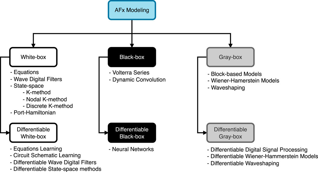
Figure 1. Audio effects modeling paradigms and methods
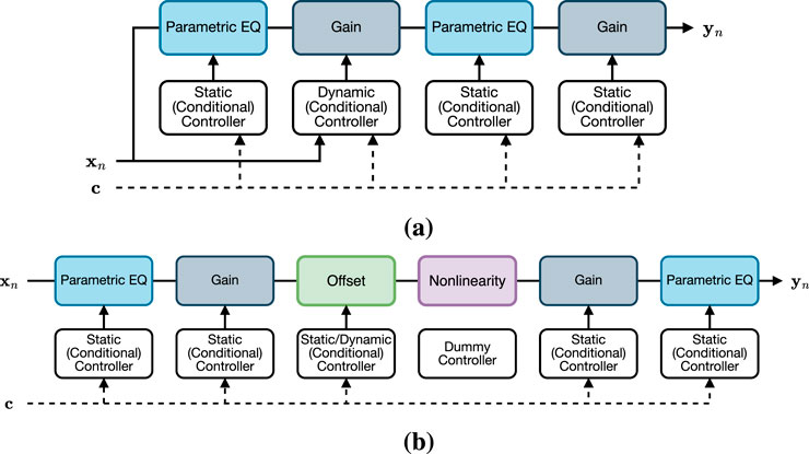
Figure 2. Proposed gray-box architectures. (a) Gray-box model for compressor/limiter. (b) Gray-box model for amp/overdrive/distortion/fuzz.
In Figure 3 we show examples of the frequency/time response learned by the proposed model when trained on a compressor (Flamma AnalogComp) and a limiter (UA 6176 Vintage Channel Strip - 1176LN Limiter). In the first example, input and output EQs differ, while in the second, a nearly symmetrical response is learned. We notice how the Dynamic Gain successfully captures different behaviors, with the compressor having slower attack and faster release than the limiter; also the exponential time constants - typical of analog compressors - appear to be correctly captured.
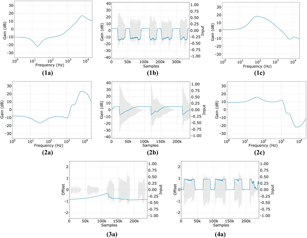
Figure 3. Examples of response for gray-box models of (1) Flamma Compressor, (2) UA 6176–1176LN Limiter, (3) Custom Dynamic Fuzz, (4) Harley Benton Fuzzy Logic. (1a) Parametric EQ. (1b) Dynamic Gain. (1c) Parametric EQ. (2a) Parametric EQ. (2b) Dynamic Gain. (2c) Parametric EQ. (3a) Dynamic Offset. (4a) Dynamic Offset
3.2.2 Model for amplifier, overdrive, distortion and fuzz
Similar to compression, there is also a wealth of literature on differentiable black-box models for: amplifiers (Covert and Livingston, 2013; Zhang et al., 2018; Schmitz and Embrechts, 2018c; Schmitz and Embrechts, 2018b; Schmitz and Embrechts, 2019; Damskägg et al., 2019a; Wright et al., 2019; Wright et al., 2020; Wright et al., 2023), overdrive (Mendoza, 2005; Ramírez and Reiss, 2019; Damskägg et al., 2019b; Wright et al., 2020; Chowdhury, 2020; Fasciani et al., 2024; Yeh et al., 2024b; Simionato and Fasciani, 2024a), distortion (Ramírez and Reiss, 2019; Damskägg et al., 2019b; Wright et al., 2019; Wright et al., 2020; Yoshimoto et al., 2020; Yoshimoto et al., 2021) and fuzz (Comunità et al., 2023). Recently, there has been exploration into applying a gray-box paradigm to this task (Kuznetsov et al., 2020; Nercessian et al., 2021; Colonel et al., 2022a; Miklanek et al., 2023; Yeh et al., 2024a), as it offers desirable characteristics such as fewer trainable parameters, greater interpretability, and reduced training data requirements.
In this work, we extend previous gray-box approaches based on the W-H model. Figure 2 illustrates our comprehensive architecture for emulating amplifiers, overdrive, distortion, and - when using dynamic controllers - fuzz effects. We use two Parametric EQs (Comunità et al., 2025) for pre- and post-emphasis filtering around a Nonlinearity, which can be memoryless or not. Gain stages control distortion and output amplitude, while an Offset stage before the nonlinearity models asymmetrical clipping. A fixed offset suffices for amplifiers, overdrive, and distortion, while a dynamic controller is needed for fuzz effects to capture hysteresis (i.e., dynamic bias shift) and the characteristic timbre during note attack and release. Conditional controllers can turn the model into a parametric one. Figure 3 shows examples of learned dynamic offsets from fuzz effects models, with the first having a longer attack and much longer release time constants than the second.
3.3 ToneTwist AFx dataset
In order to establish the state of the art in audio effects modeling across various effect types, we required access to dry-input/wet-output data from multiple devices; and, since modeling mainly focuses on physical units, data needed to be from analog devices. For a realistic scenario, data needed to include a variety of sources, content and playing techniques, to test generalization capabilities beyond the ones used for training. Furthermore, to run extensive experiments efficiently, we needed consistently organized data to avoid custom preprocessing and dataset code for each device.
Although there are publicly available datasets for audio effects modeling (Stein et al., 2010; Comunità et al., 2021; Pedroza et al., 2022), these were deemed unsuitable for our work for several reasons. The IDMT-SMT-Audio-Effects6 (Stein et al., 2010) dataset focuses on detection and classification tasks, it is limited to single notes and chords from two electric guitars and two electric basses, and it only includes digital effects covering 10 linear, non-linear, and modulation effects. Similarly, GUITAR-FX-DIST (Comunità et al., 2021), which focuses on classification and parameter estimation, includes single notes and chords from two guitars and only features digital emulations of 14 distortion effects. While EGFxSet7 (Pedroza et al., 2022) includes recordings from 12 physical units, equally split between analog and digital, it only features single notes from one electric guitar; and, despite being intended for audio effects modeling, it is unsuitable due to high background noise and other artifacts.
For the reasons above, we introduce the ToneTwist AFx dataset8 (Table 1), the largest collection (40 devices at the time of writing) of dry/wet signal pairs from nonlinear audio effects. Beside being the first thoroughly documented audio effects dataset, it is also open to contributions from the wider community. While data is hosted on Zenodo9 for long-term availability, our repository organizes download links, provides retrieval scripts, basic training code, and contribution guidelines, facilitating new submissions and fostering discussion.
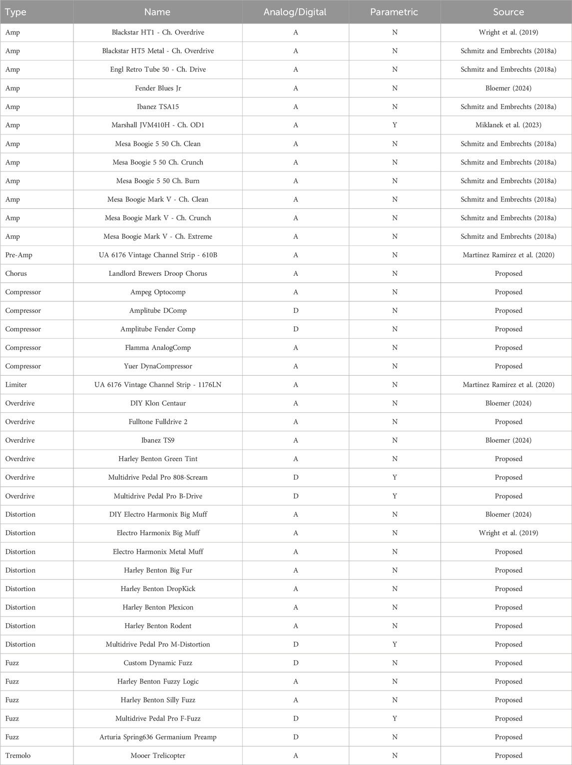
Table 1. ToneTwist AFx Dataset (at the time of writing). For accessibility, we also include data from previous works (see Source) which we verify, pre-process (when necessary), rename, and reorganize for consistency.
ToneTwist AFx is organized into four categories: analog, analog parametric, digital, and digital parametric, with parametric referring to entries sampled with control settings granularity sufficient for parametric modeling. It features dry-input signals from seven sources, including a variety of guitars, basses, and test signals like chirps and white noise. The test set features different content and instruments from the training/validation set, ensuring a realistic evaluation of the generalization capabilities of trained models.
Recording was carried out with a Focusrite Scarlett Solo audio interface, featuring a low-noise pre-amplifier (
4 Experiments
In this section we give an overview and description of all the architectures, models configurations, and data used for our experiments. To help establish the state of the art in audio effects modeling and identify future research directions, we included a wide range of experiments and configurations.
4.1 Overview of models configurations
Table 2 lists all models, hyperparameter values, and computational complexity10 used in our experiments on non-parametric modeling, where we balance tractability by limiting the number of models per architecture while covering a broad range of sizes and complexities.
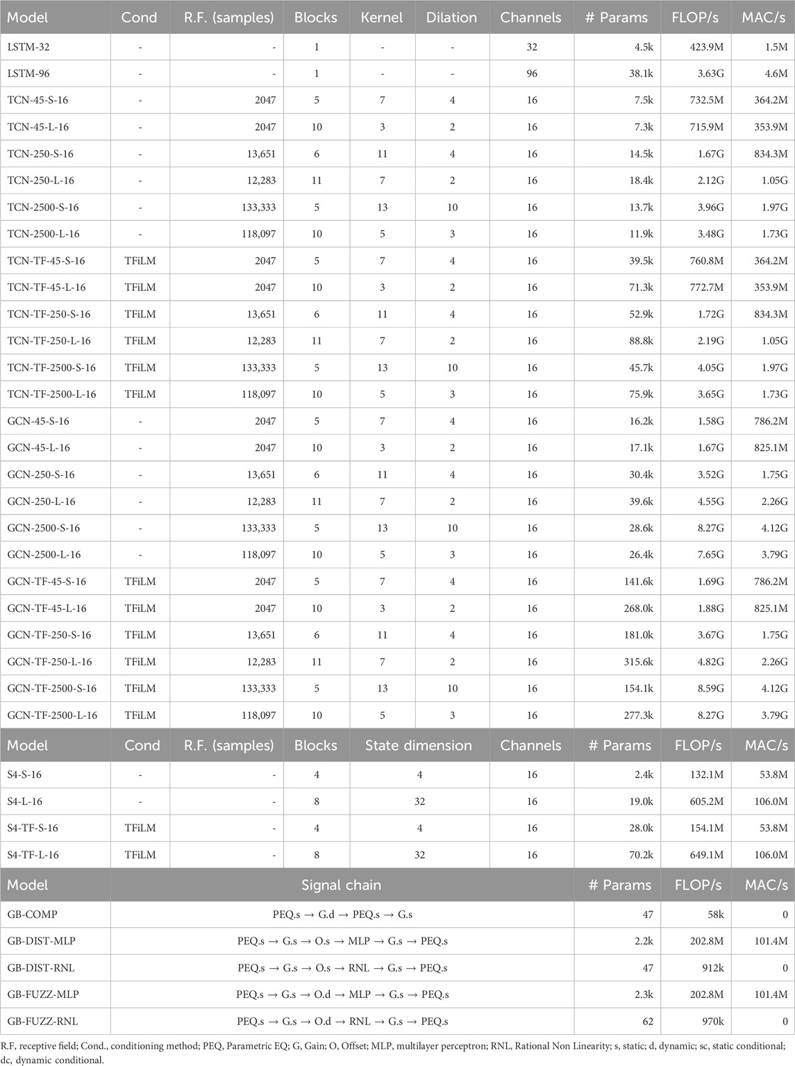
Table 2. Configurations for models included in the experiments.
As described in Section 3.1, we include the four most common neural networks types for black-box modeling: LSTM, TCN, GCN and S4; as well as the gray-box models proposed in Section 3.2: GB-COMP for compressor/limiter, GB-DIST for amplifier/overdrive/distortion and GB-FUZZ for fuzz. For LSTM architectures, the only parameter to choose is the number of channels, with 32 and 96 channels being sensible choices for small and large models (LSTM-32/LSTM-96), as adopted in previous works Wright et al. (2020); Steinmetz and Reiss (2022); Comunità et al. (2023).
For TCN and GCN models, we consider variants with short, medium, and long receptive fields (45, 250 and 2,500 ms at 48 kHz), with small (5/6 blocks) or large (10/11 blocks) configurations (S/L in model names). We keep the number of channels constant and equal to 16. We also include variants without and with TFiLM (TF in the models’ names) to evaluate whether time-varying conditioning - shown to be able to capture long-range dependencies (Comunità et al., 2023) typical of compressors and fuzz effects - is beneficial across architectures. For TFiLM layers we always adopt a block size - i.e., downsampling/maxpooling factor - of 128, which was shown to be optimal in (Comunità et al., 2023). As shown in the table, for each receptive field, small and large models have comparable parameters, FLOP/s, and MAC/s, with the idea that the main difference is in the number of processing stages and not in the networks expressivity itself. With TFiLM adding a conditioning layer per block, matching parameter counts across block variations isn’t feasible, but due to the small channel count (16) and low TFiLM sample rate, model pairs remain computationally comparable.
For S4 architectures we define small and large models (S/L in the name) based on the number of blocks and state dimension, with values chosen based on the experiments reported in the original publication (Gu et al., 2021a). For S4 models as well we introduce TFiLM conditioned variants and keep the number of channels constant and equal to 16.
While for the GB-COMP architecture we only investigate one configuration, for GB-DIST and GB-FUZZ models we test two, based on the type of nonlinearity adopted: Static MLP Nonlinearity or Static Rational Nonlinearity (MLP/RNL in the name). The MLP itself accounts for most of the computational complexity of GB-DIST and GB-FUZZ models.
For experiments on parametric modeling (Table 3) we take a subset of the configurations in Table 2 and we pair them with the various conditioning mechanisms described in (Comunità et al., 2025). For LSTM models, we use concatenation (C) as the baseline and also test time-varying concatenation (TVC), which adds minimal computational cost. For convolutional backbones, we select only TCNs and models with a short (45 ms) receptive field, as these rely more on conditioning methods to capture long-range dependencies, highlighting performance differences. We consider FiLM conditioning (F in the name) to be the baseline method and experiment with TFiLM, TTFiLM (TTF in the name) and TVFiLM (TVF in the name). We do the same for S4 architectures. Table 3 shows that both TTFiLM and TVFiLM introduce time-dependent conditioning with parameter and computational efficiency similar to the baseline FiLM method, having minimal impact on parameters, FLOP/s, and MAC/s. For gray-box models, we add parametric control using differentiable controllers from (Comunità et al., 2025) and replace static/dynamic controllers with conditional ones (C in the model name). Although they increase the number of parameters, the impact of conditional controllers on the computational complexity is minimal due to the small size of the MLPs and LSTMs in their implementation.
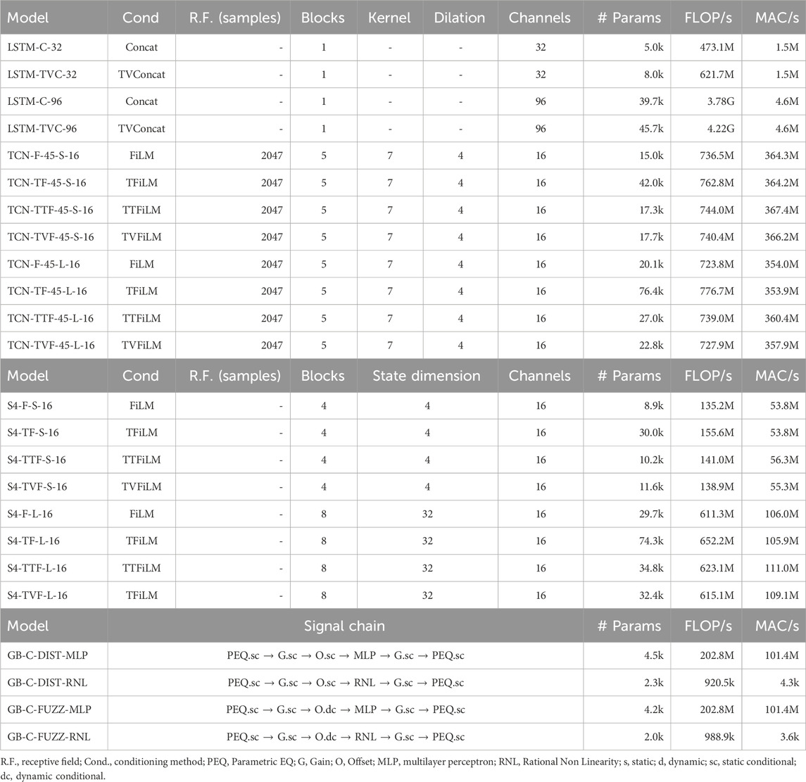
Table 3. Configurations for models included in the experiments.
Beside a good understanding of the state-of-the-art, our experiments aim to identify architectures that can model a wide range of effects and devices consistently, without requiring different configurations, with the broader goal of defining a universal audio effects modeling architecture. While we recognize that model pruning (Südholt et al., 2022) or hyperparameter optimization could identify the smallest model size for each effect, this would require extensive time and resources. Alternatively, model distillation (Hinton et al., 2015) could reduce size and increase efficiency after identifying a suitable architecture, but this also requires additional experimentation and training.
4.2 Overview of audio effects configurations
Table 4 lists all the audio effects and settings in our study. For non-parametric modeling, we select four devices per effect category (compressor/limiter, overdrive, distortion, fuzz), totaling sixteen devices, twelve of which are from our ToneTwist AFX dataset (see Section 3.3).
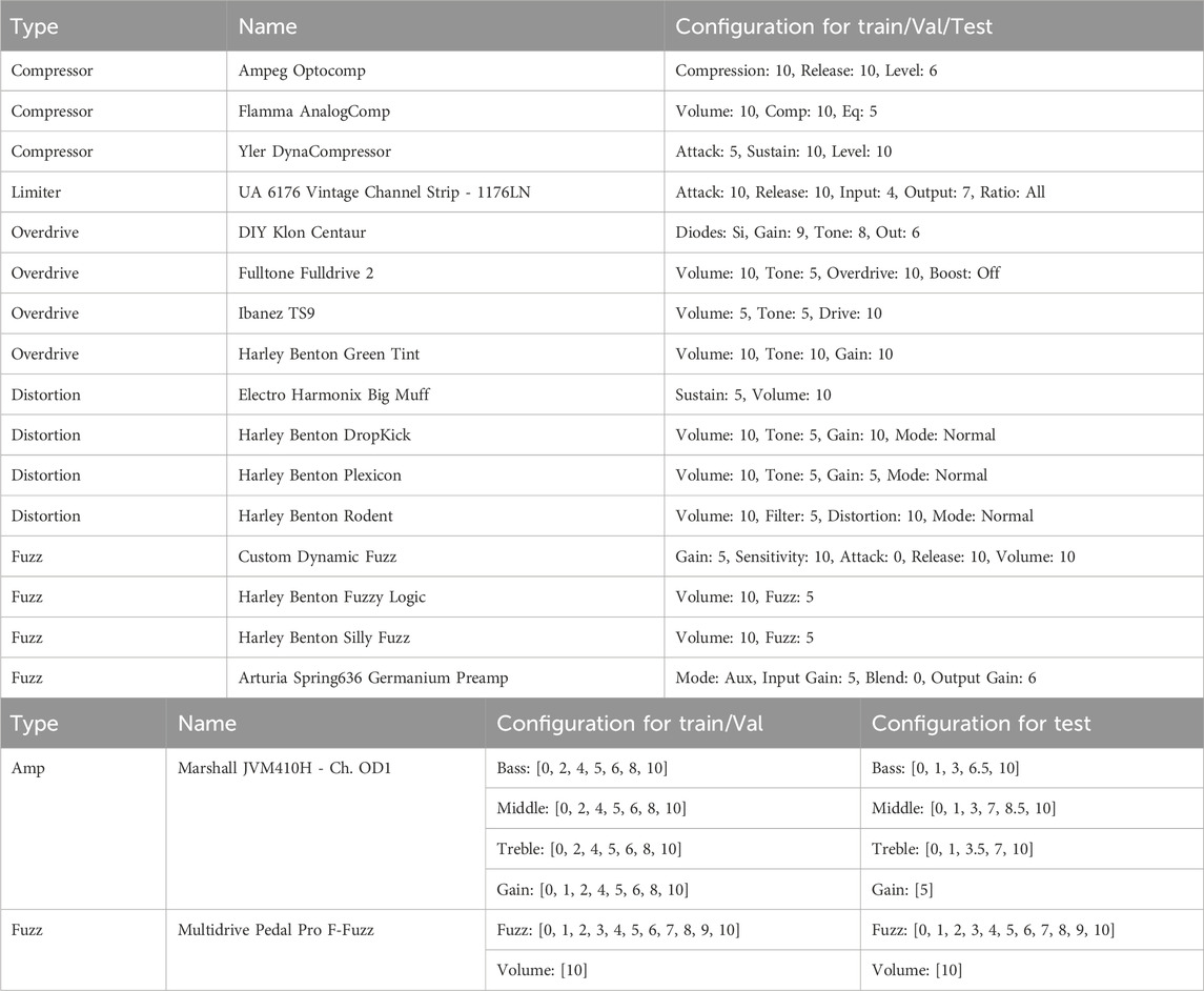
Table 4. Audio effects configurations use in the experiments. For parametric models not all combinations are part of the data.
Settings for each device are chosen to ensure a variety of behaviors within each category, while maximizing the challenge for the modeling task. For compression, we select fast attack, slow release, and high compression ratio settings to capture fast transients, long-range dependencies, and nonlinear behaviors. For overdrive, we choose high gain settings with varying tone/equalization for a complex spectrum. For distortion, we select both medium and high gain settings, while for fuzz effects, which are inherently high gain, we opt for medium gain settings to ensure the dynamic behavior is noticeable and not concealed by excessive distortion. It is important to note that the settings values across effect types and devices are only vaguely correlated with the behaviors we are modeling, as they don’t correspond to specific units or internal parameters, serving only as a general description of the effect’s behavior and timbral traits.
The table also includes effects and settings for parametric modeling experiments: a vacuum tube guitar amplifier and a digital germanium transistor fuzz emulation. In addition to parametric modeling and conditioning methods, data from these two devices help evaluate performance on unseen control configurations and sources. For the Marshall JVM410H, training, validation, and testing use the same sources but different control settings. For the Multidrive Pedal Pro F-Fuzz, control settings are the same across sets, but sources and content differ, featuring unseen guitar and bass performances.
4.3 Training
Many previous audio effects modeling studies have typically assumed that training different architectures and model configurations under a consistent training scheme—including loss functions, loss weights, learning rate, and scheduler—provides a reasonable basis for performance comparison and drawing conclusions about state-of-the-art approaches. This has been the case also for works that compared vastly different architectures like black-box and gray-box ones (Yeh et al., 2024a; Miklanek et al., 2023; Wright and Valimaki, 2022). Although, in preliminary experiments we were able to assess that training an architecture under different schemes can yield vastly different loss values, and even more so when different architectures are involved. This highlights the need to choose appropriate training-related hyperparameters for each model to enable meaningful comparisons between architectures and configurations.
This section discusses preliminary experiments to identify optimal hyperparameters and training configurations for LSTM, TCN, GNC, S4, and GB architectures, and the resulting training schemes are shown in Table 5. Based on prior work on effects modeling Steinmetz and Reiss (2022); Comunità et al. (2023), sound synthesis Engel et al. (2019), and audio processing (Yamamoto et al., 2020), we assumed an
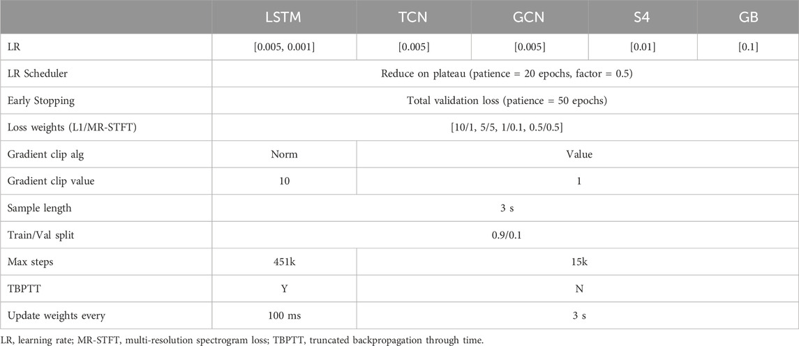
Table 5. Training configurations for each architecture.
We chose the learning rate (LR) for each architecture by training on one audio effect (Custom Dynamic Fuzz) and comparing results for
A major challenge during this phase was the instability in training LSTM models, resulting in frequent gradient explosion failures despite adjustments to: LR, gradient clipping, loss weights, training samples length, and the use of truncated backpropagation through time (TBPTT) (Comunità et al., 2025). A suboptimal solution was to select the training scheme reported in Table 5. While this does not prevent NaN loss failures, it helps to reach a suitable local optimum by training each model with a broader range of hyperparameters. For TBPTT, gradients are updated every 4,800 samples (100 ms at 48 kHz), and the max training steps match the epochs used for models without TBPTT. All other architectures revealed to be much more stable - with no NaN loss cases - while still benefiting from training on a variety of LRs to achieve optimal results. For all architectures we opt to reduce LR by half when there are no improvements in total validation loss for 20 epochs. To prevent overfitting, we also use early stopping of 50 epochs.
Examples that highlight differences in performance as a function of LR are shown in Figure 4, with training sessions that might not reach a good local optimum (Figure 4a) or exhibit scaled-loss differences of up to 30%–40% (Figures 4b,c).

Figure 4. Validation scaled-loss for different learning rates reveals training discrepancies and unreliability of previous literature comparing architectures and model configurations using a single training scheme. (a) LSTM trained on Harley Benton Plexicon. (b) S4 trained on Harley Benton Rodent (c) GB-FUZZ trained on Harley Benton Fuzzy Logic.
5 Results
5.1 Results for non-parametric models
Figure 5 shows the total loss for architectures trained on sixteen effects (see Section 4), with box plots for overall results (Figure 5a) and each effect category (Figures 5b-e).
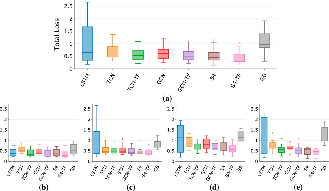
Figure 5. Total loss for different architectures: overall and for each effect type. (a) Overall. (b) Compressor/Limiter (c) Overdrive (d) Distortion (e) Fuzz.
Overall, S4 models with TFiLM conditioning perform the best. Also, TFiLM improves median performance across architectures and reduces the variance, demonstrating how time-varying conditioning enhances expressivity, regardless of the backbone. Although GCN achieves lower loss than TCN, TFiLM conditioning results in similar performance for both, making the added complexity of GCN-TF hard to justify and emphasizing how efficient and effective time-varying conditioning could be focus of further research. Gray-box models show higher median loss than black-box ones but can outperform them in some cases, and also exhibit smaller variance than LSTMs. Having the greatest variance across architectures, LSTMs are shown to be the least reliable, which makes them unsuitable for modeling a wide range of effect types and devices.
Breaking down performance by effect type, S4 models perform best in each category, with TFiLM conditioning generally improving or maintaining performance without hindering it. It therefore seems that S4 models with a form of time-dependent conditioning are the best candidate to develop high performing architectures across a wide range of effect types and implementations.
In convolutional architectures, TFiLM is shown to be helpful for every effect category although to a varying extent, particularly benefiting distortion and fuzz effects with their complex timbre and time-dependent behaviors. This is reflected in the average loss and standard deviation in Table 6, where distortion and fuzz are the most challenging effects to model. Beside compressors, LSTM is confirmed to be the least reliable architecture in each category, with far greater variance than any other architecture and performing on par or worse than gray-box models.
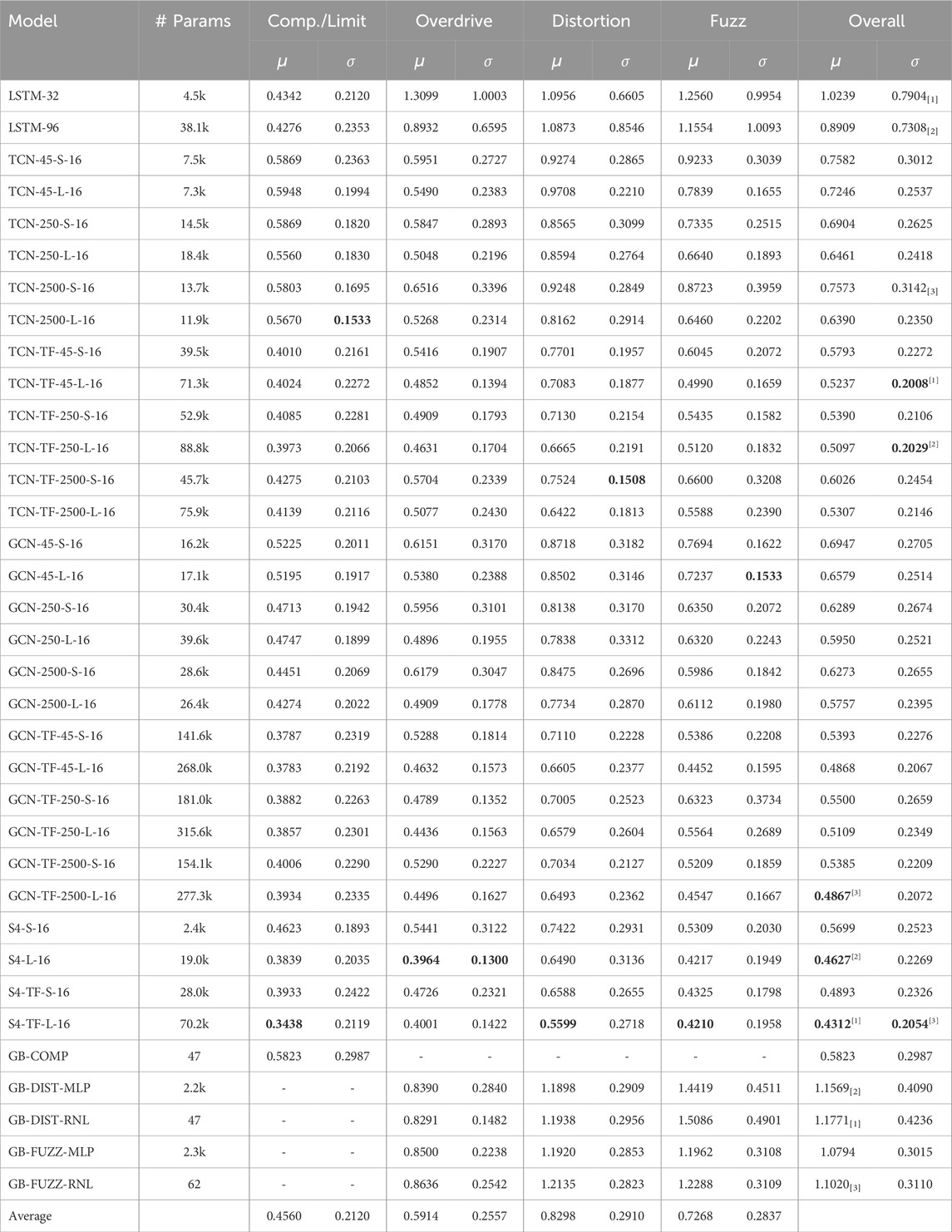
Table 6. Mean
Looking in further details at the results in Table 6 where we gather mean
5.2 Results for parametric models
Table 7 shows the losses for parametric models trained on Marshall JVM410H guitar amplifier and Multidrive Pedal Pro F-Fuzz digital emulation of Fuzz Face guitar pedal. We report both validation and test loss to assess model performance when tested on unseen controls configurations (i.e., guitar amp) or unseen sources and content (i.e., fuzz pedal). S4 models are the best performing on the guitar amp, with LSTM models and TCN with time-varying conditioning performing only marginally worse. For the fuzz effect pedal emulation, LSTMs are the best performing, with S4 models with time-varying conditioning (S4-TF-L-16 and S4-TVF-L-16) being only slightly worse.
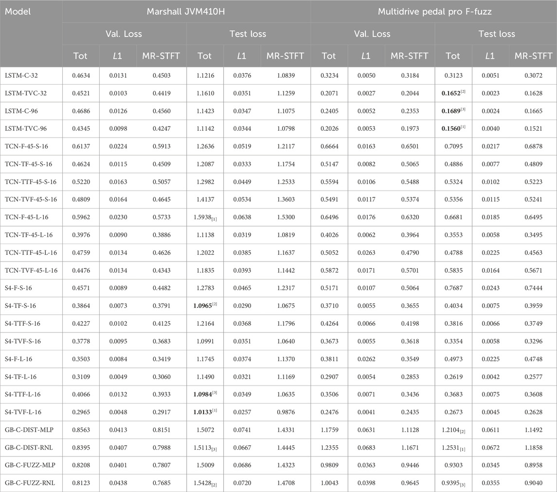
Table 7. Mean
While TVCond (TVC) conditioning is not useful to improve LSTM performance on the Marshall amp, it is beneficial to achieve among best performance with a smaller LSTM model. For TCN models, TFiLM (TF) conditioning is the most effective for both guitar amp and fuzz pedal cases, regardless of the number of layers in the model. We also notice how the baseline FiLM (F) conditioning is the worst mechanism for all but one case when applied to either TCN or S4 models. Looking at S4 models, the proposed TTFiLM (TTF) and TVFiLM (TVF) conditioning allow performance on par or better than TFiLM (TF) regardless of model size. Also, TVF allows small models to achieve performance comparable to bigger ones. For TCN models, it is less clear whether there is an advantage in using TTF or TVF w.r.t. TF beside computational complexity.
To recap, TFiLM seems to be the best across architectures, with TVFiLM better than TTFiLM when reducing the computational complexity. A study on a wider variety of effects would allow to better asses whether TVF and TTF can compete with TF conditioning.
6 Evaluation
6.1 Objective evaluation
To extend the objective evaluation beyond loss values we use most of the metrics available from the NablAFx framework (Comunità et al., 2025), these include both signal-based metrics (i.e., MSE, ESR, MAPE) as well as latent representation-based ones (i.e., FAD). FAD is computed using three widely adopted representations (i.e., VGGish, PANN and CLAP) as well as a recently proposed audio production style representation (AFx-Rep) Steinmetz et al. (2024). We compute these metrics for several reasons beside broadening the analysis: to investigate which ones might be most suited for modeling tasks, to investigate correlation between objective metrics and subjective ratings (see Section 6.4), to encourage further research on audio effects related representations and evaluation methods.
When using objective metrics - which we plot in Figures 6, 7 on a log scale to highlight differences - the picture is similar to the results discussed in previous sections. S4 and S4-TF architectures show the best performance across effect type, regardless of the metric used. Once again, temporal conditioning (TFiLM), is helpful in improving performance - noticeable from the reduction in median as well as standard deviation values - regardless of the architecture’s backbone (TCN, GCN or S4). LSTM architectures are shown again to have a high performance variance, making them not reliable when modeling a wide range of devices. While gray-box models again achieve results that are not on par with black-box ones, therefore requiring further exploration.
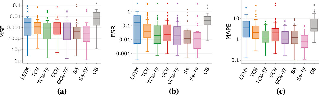
Figure 6. Metrics for different architectures for all effect types. (a) MSE. (b) ESR. (c) MAPE.
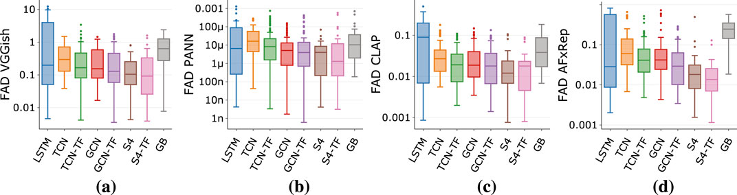
Figure 7. FAD for different architectures for all effect types. (a) VGGish. (b) PANN (c) CLAP (d) AFx-Rep.
6.2 Efficiency
While a full performance evaluation is beyond the scope of this work, we investigated the run-time of the proposed models and conditioning methods in a frame-based implementation to mimic a standard digital audio effect implementation.
The real-time factor (RTF) is defined as:
where
Results for non-parametric models are shown in Figures 8A,B and for parametric ones in Figure 8C. We show only a limited number of configurations for clarity. In a block-based formulation, TCN models require a buffer of past samples such that we pass an input of
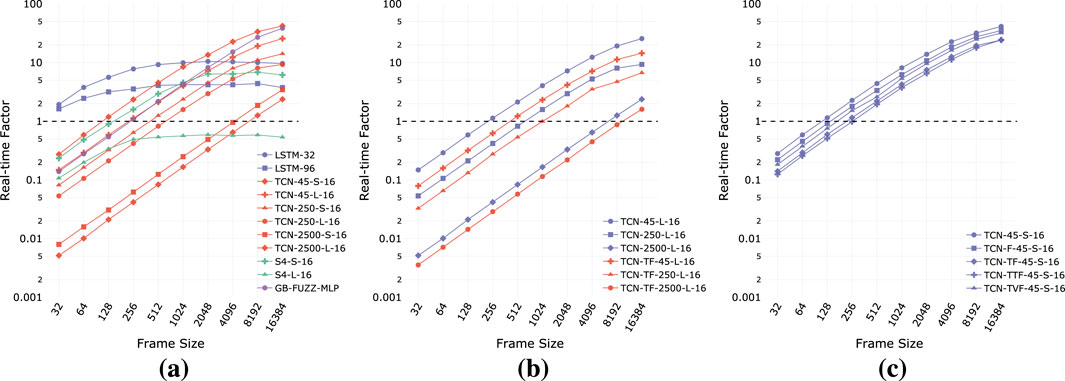
Figure 8. Real-time factor vs Frame size for some of the models included in the experiments. (a) Architectures. (b) Receptive field. (c) Conditioning method.
LSTMs achieve real-time operation at every frame size, but the RTF remains constant over a certain size due to the inability to parallelize computations along the temporal dimension. The RTF for TCN, GCN (not shown) and GB models, is instead proportional to the frame size. For convolutional backbones, whether the models achieve real-time operation at a sufficiently small frame size is strongly related to the receptive field and the number of blocks. Interestingly, S4 models show a behavior in between recurrent and convolutional networks, where the RTF is proportional to frame size for small sizes and flattens out for large sizes. Although best performing, S4 models require appropriate choice of number of blocks and state dimension to allow real-time operation, in fact, our larger model does not achieve
Figure 8B compares TCN models with and without TFiLM conditioning, with temporal feature-wise modulation consistently reducing the RTF at every model and frame size. Also, in Figure 8C we compare different conditioning methods (FiLM, TFiLM, TTFiLM, TVFiLM) for parametric TCN models, and include a non-parametric model (TCN-45-S-16) for reference. We notice how, even if computationally as efficient as models with FiLM and TVFiLM, TTFiLM conditioning is the worst in terms of RTF, while TVFiLM achieves real-time performance between FiLM and TFiLM, introducing time-varying conditioning at a low computational cost.
We emphasize, however, that RTF alone does not fully capture the suitability of a model for real-time audio deployment. Factors such as latency, system-level I/O delays, and the implementation environment (e.g., Python vs C++) significantly affect overall performance. Our results should therefore be interpreted as a lower-bound indication of computational cost under a reference implementation, rather than a definitive real-time capability assessment.
6.3 Summary
In Figure 9, we present a summary of our experimental results by plotting the mean total loss (L1 + MR-STFT) across all devices for each model configuration. Different architectures are distinguished by color, and marker sizes are scaled according to model complexity, calculated as the sum of parameters, FLOPs, and MACs. Additionally, the real-time factor (RTF), computed for a frame size of 512 samples, is displayed above each marker, with values equal or greater than one shown in bold.
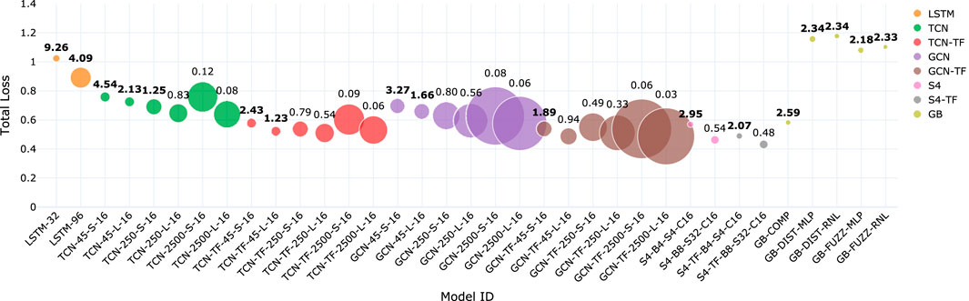
Figure 9. Mean total loss (L1 + MR-STFT) across all devices for each model included in our experiments. Color indicates different architectures. Marker size proportional to model complexity (# Params + FLOP/s + MAC/s). Numbers above each marker show the real-time factor for a frame size of 512 samples. Bold indicates models for which the real-time factor is equal or greater than 1.
This figure highlights several key findings from our experiments. Large S4 models achieve the highest accuracy but exhibit lower efficiency compared to other architectures, despite their design intent to leverage CNNs’ training efficiency and RNNs’ inference efficiency (see Section 2.5). Notably, S4 models show significantly lower real-time factors (RTF) than LSTM models, raising questions about their practical inference efficiency. TFiLM conditioning consistently improves accuracy across all backbones (TCN, GCN, S4), with only a marginal increase in computational complexity, although it introduces a measurable reduction in efficiency. Models with long receptive fields (TCN and GCN) suffer from high computational costs, while applying TFiLM to architectures with short receptive fields appears to be a more efficient strategy for modeling long-range dependencies characteristic of dynamic range compression and fuzz effects. Additionally, the increased complexity of GCNs over TCNs does not yield proportional accuracy gains, with TFiLM conditioning providing a more effective improvement. Finally, gray-box models—except GB-COMP, which performs comparably to black-box baselines—do not yet offer clear advantages in accuracy or efficiency, suggesting that more advanced designs may be needed to fully realize the potential of theoretically grounded architectures like those based on Wiener-Hammerstein models.
6.4 Subjective evaluation
To evaluate the perceptual differences among architectures, we conducted a MUSHRA listening test, and the participants provided written informed consent to participate in this study.
Each trial presented participants with processed audio from all architectures under evaluation (LSTM, TCN, TCN-TF, GCN, GCN-TF, S4, and S4-TF) alongside a reference signal (wet-output) and an anchor (dry-input). We selected 12 effects (3 per type) out of the 16 we trained on. For each effect, we curated three distinct sound examples designed to highlight model performance. These included a bass riff with a high input level and clear attacks to emphasize timbral and temporal characteristics, a guitar sample at similarly high input levels with pronounced attacks to further assess these aspects, and a second guitar sample with a very low input level and steady picking. This last example was chosen to evaluate the models’ ability to faithfully capture devices across extreme input dynamics.
For each architecture we selected the best-performing model in terms of total test loss. The listening test consisted of a total of 68 possible questions, with each participant randomly assigned seven to maintain a manageable test duration. A total of 27 participants were recruited, and a rigorous screening process was implemented. Participants were assessed on prior experience with listening tests, musical training or production experience, and familiarity with the specific effects being evaluated (compressors, overdrive/distortion, and fuzz). Further filtering was applied to ensure test reliability, participants who did not rate the reference sample at 80 or higher in more than one out of their seven trials were excluded from the final analysis. After applying these screening criteria, we obtained 350 valid ratings in total, averaging 35 per architecture and approximately 8.75 ratings per effect type. Our strict participant selection strategy was intentional, prioritizing fewer but highly skilled listeners. This approach significantly reduced rating variance, leading to a more reliable subjective evaluation of model performance.
We show the overall results in Figure 10 together with ratings broken down by effect category. In general, subjective ratings confirm the results obtained during the training process, with S4 architectures performing best, followed by convolutional backbones, gray-box models and LSTMs. TFiLM conditioning allows to increase median accuracy and lower variance, improving modeling reliability across effects types and devices. With respect to objective metrics, gray-box models are on average rated higher than LSTMs, but with high variance, which might entail the potential to match black-box approaches while requiring careful architecture design for different effect types. Once again, LSTMs are confirmed to be unreliable as modeling architectures on a wide range of devices.
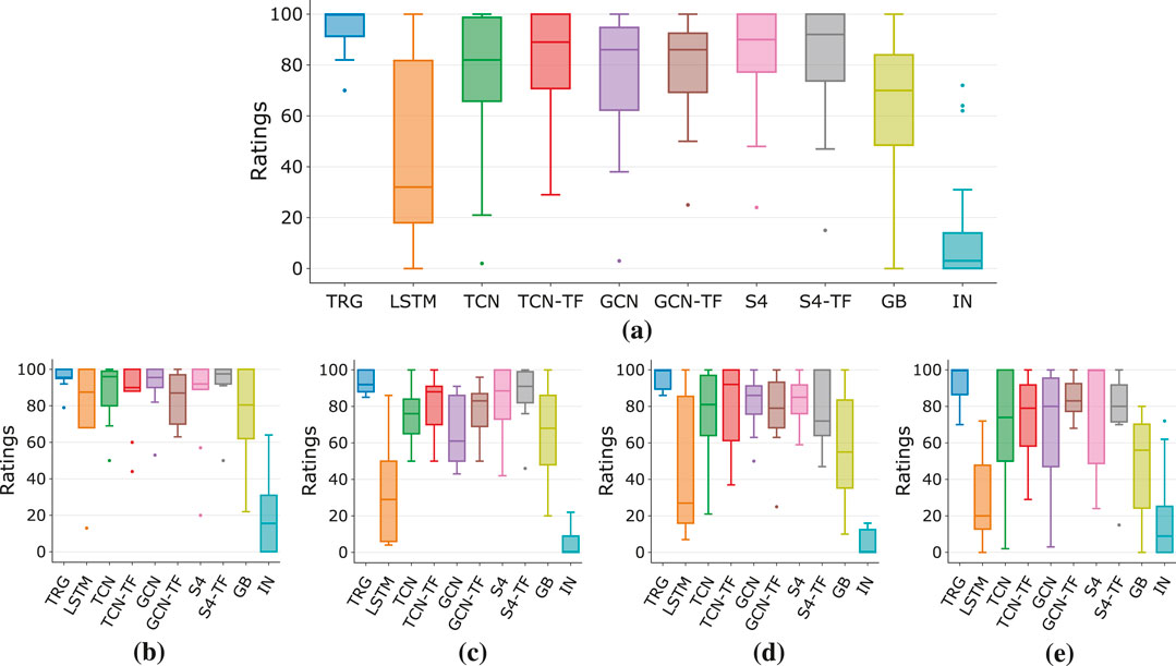
Figure 10. Subjective ratings for different architectures: overall and for each effect type. (a) Overall. (b) Compressor/Limiter. (c) Overdrive. (d) Distortion. (e) Fuzz.
If we break down ratings by effect type we notice that in the majority of cases TFiLM helps to improve performance, in particular for convolutional backbones trained on overdrive, distortion and fuzz. Proposed gray-box models perform, on average, well on compression and fairly on overdrive, while less so on distortion and fuzz. Also, GCNs are not consistently better than TCNs, which confirms that the added complexity of GCNs is in general not necessary for good performance. S4 models remain the most consistent, with median ratings at or above 80 in all but one case.
6.5 Correlation
We further extend our analysis calculating the Spearman correlation between objective metrics and subjective ratings (Table 8). Out of the signal-based metrics, MR-STFT shows the highest correlation with human ratings, supporting the assumption that it is a suitable term to include in the loss function. MAPE and L1 are the second and third most correlated metrics, again supporting the idea that including a time-domain loss term is meaningful for modeling tasks. Considering effects type, MR-STFT is the most relevant for high-distortion effects, while MAPE and L1 are the most correlated with subjective ratings for overdrive and compression respectively, although in the latter case, absolute correlation values are very low or not significant
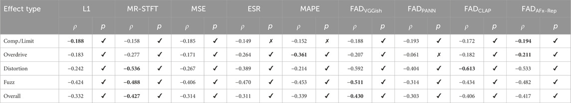
Table 8. Spearman correlation
Observing latent representation-based metrics instead, VGGish and AFx-Rep vectors are overall the most correlated with subjective ratings. Looking at specific effect types, none of the representations seem to be suited for compression and overdrive models evaluation, while CLAP and VGGish are, respectively, highly correlated with distortion and fuzz effects.
7 Conclusions and future work
In this work, we conducted extensive experiments to establish the state of the art in differentiable black-box and gray-box approaches for nonlinear audio effects modeling. Our study explored task-specific neural network architectures, proposed differentiable DSP-based gray-box models, and presented ToneTwist AFx, a large dataset of dry-input/wet-output pairs for audio effects research.
We described the challenges of training and comparing different approaches, and demonstrated how careful consideration of the training scheme is essential to ensure fair comparisons and draw reliable conclusions.
Thanks to our extensive objective and subjective evaluations we concluded that state-space models are the most suited to model a wide range of devices, with TCN and GCN architectures also achieving very good results. We found LSTM-based recurrent networks to be unreliable across devices and DDSP-based models not yet on par with neural networks. Time-varying conditioning like TFiLM was proven beneficial, across convolutional and state-space backbones, to improve median and variance in objective metrics and subjective ratings. Our analysis of the correlation between subjective ratings and signal-based metrics showed that a loss function combining time-domain (L1/MAPE) and spectro-temporal-domain (MR-STFT) is generally effective. However, there is room for improvement in signal-based and latent representation-based metrics for model evaluation.
Given these results, future work might focus on any of the following aspects:
Data availability statement
The datasets presented in this study can be found in online repositories. The names of the repository/repositories and accession number(s) can be found below: https://github.com/mcomunita/tonetwist-afx-dataset.
Ethics statement
The participants provided written informed consent to participate in this study.
Author contributions
MC: Conceptualization, Data curation, Formal Analysis, Investigation, Methodology, Project administration, Resources, Software, Validation, Visualization, Writing – original draft, Writing – review and editing. CS: Software, Supervision, Writing – review and editing. JR: Supervision, Writing – review and editing.
Funding
The author(s) declare that financial support was received for the research and/or publication of this article. Funded by UKRI and EPSRC as part of the “UKRI CDT in Artificial Intelligence and Music”, under grant EP/S022694/1.
Conflict of interest
The authors declare that the research was conducted in the absence of any commercial or financial relationships that could be construed as a potential conflict of interest.
Generative AI statement
The author(s) declare that no Generative AI was used in the creation of this manuscript.
Publisher’s note
All claims expressed in this article are solely those of the authors and do not necessarily represent those of their affiliated organizations, or those of the publisher, the editors and the reviewers. Any product that may be evaluated in this article, or claim that may be made by its manufacturer, is not guaranteed or endorsed by the publisher.
Supplementary Material
The Supplementary Material for this article can be found online at: https://www.frontiersin.org/articles/10.3389/frsip.2025.1580395/full#supplementary-material
Footnotes
1https://github.com/mcomunita/tonetwist-afx-dataset
2https://github.com/mcomunita/nablafx
3https://github.com/mcomunita/nnlinafx-supp-material
4https://ccrma.stanford.edu/∼dtyeh/papers/wdftutorial.pdf
5https://github.com/mcomunita/nablafx
6https://www.idmt.fraunhofer.de/en/publications/datasets/audio_effects.html
8https://github.com/mcomunita/tonetwist-afx-dataset
10https://github.com/MrYxJ/calculate-flops.pytorch
References
Bai, S., Kolter, J. Z., and Koltun, V. (2018). An empirical evaluation of generic convolutional and recurrent networks for sequence modeling. arXiv preprint arXiv:1803.01271. doi:10.48550/arXiv.1803.01271
Bank, B. (2011). “Computationally efficient nonlinear Chebyshev models using common-pole parallel filters with the application to loudspeaker modeling,” in Audio Engineering Society Convention 130, London, UK, May 13–16 2011.
Bengio, Y., Goodfellow, I., and Courville, A. (2017). Deep learning, vol. 1. Cambridge, MA, USA: MIT press.
Bernardini, A., and Sarti, A. (2017). Biparametric wave digital filters. IEEE Trans. Circuits Syst. I Regul. Pap. 64, 1826–1838. doi:10.1109/tcsi.2017.2679007
Bernardini, A., Vergani, A. E., and Sarti, A. (2020). Wave digital modeling of nonlinear 3-terminal devices for virtual analog applications. Circuits, Syst. Signal Process. 39, 3289–3319. doi:10.1007/s00034-019-01331-7
Birnbaum, S., Kuleshov, V., Enam, Z., Koh, P. W. W., and Ermon, S. (2019). Temporal film: capturing long-range sequence dependencies with feature-wise modulations. Adv. Neural Inf. Process. Syst. 32. doi:10.48550/arXiv.1909.06628
Blair, J. (2015). Southern California surf music, 1960-1966. Mount Pleasant, SC: Arcadia Publishing.
Bloemer, K. (2024). GuitarML. Available online at: https://github.com/GuitarML (Accessed November 15, 2024).
Bogason, Ó. (2018). Modeling auto circuits containing typical nonlinear components with wave digital filters. Canada: McGill University.
Bogason, Ó., and Werner, K. J. (2017). “Modeling circuits with operational transconductance amplifiers using wave digital filters,” in Proc. of the Int. Conf. on Digital Audio Effects DAFx-17, 5th - 9th Sept 2017.
Borquez, D. A. C., Damskägg, E.-P., Gotsopoulos, A., Juvela, L., and Sherson, T. W. (2022). Neural modeler of audio systems.
Carini, A., Cecchi, S., Romoli, L., and Sicuranza, G. L. (2015). Legendre nonlinear filters. Signal Process. 109, 84–94. doi:10.1016/j.sigpro.2014.10.037
Carini, A., Orcioni, S., Terenzi, A., and Cecchi, S. (2019). Nonlinear system identification using wiener basis functions and multiple-variance perfect sequences. Signal Process. 160, 137–149. doi:10.1016/j.sigpro.2019.02.017
Cauduro Dias de Paiva, R., Pakarinen, J., and Välimäki, V. (2012). “Reduced-complexity modeling of high-order nonlinear audio systems using swept-sine and principal component analysis,” in 45th International Audio Engineering Society Conference, Helsinki, Finland, March 1-4, 2012.
Chowdhury, J. (2020). A comparison of virtual analog modelling techniques for desktop and embedded implementations. arXiv preprint arXiv:2009.02833. doi:10.48550/arXiv.2009.02833
Chowdhury, J., and Clarke, C. J. (2022). “Emulating diode circuits with differentiable wave digital filters,” in Proceedings of the 19th sound and music computing conference (Saint-Etienne, France: Zenodo).
Cohen, I., and Hélie, T. (2010). “Real-time simulation of a guitar power amplifier,” in Proc. of the Int. Conf. on Digital Audio Effects (DAFx-10), Graz, Austria, September 6-10, 2010.
Colonel, J., and Reiss, J. D. (2022). “Approximating ballistics in a differentiable dynamic range compressor,” in Audio Engineering Society Convention 153, New York, USA, 19-20 October 2022.
Colonel, J. T., Comunità, M., and Reiss, J. (2022a). “Reverse engineering memoryless distortion effects with differentiable waveshapers,” in Audio Engineering Society Convention 153, New York, USA, 19-20 October 2022.
Colonel, J. T., and Reiss, J. (2023). Reverse engineering a nonlinear mix of a multitrack recording. J. Audio Eng. Soc. 71, 586–595. doi:10.17743/jaes.2022.0105
Colonel, J. T., Steinmetz, C. J., Michelen, M., and Reiss, J. D. (2022b). “Direct design of biquad filter cascades with deep learning by sampling random polynomials,” in 2022 IEEE International Conference on Acoustics, Speech and Signal Processing (ICASSP), Singapore, 23-27 May 2022, 3104–3108. doi:10.1109/icassp43922.2022.9747660
Comunita, M., and Reiss, J. D. (2024). “Afxresearch: a repository and website of audio effects research,” in DMRN+ 19: digital music research network one-day workshop 2024.
Comunità, M., Steinmetz, C. J., Phan, H., and Reiss, J. D. (2023). “Modelling black-box audio effects with time-varying feature modulation,” in 2023 IEEE international conference on acoustics, speech and signal processing (ICASSP). doi:10.1109/ICASSP49357.2023.10097173
Comunità, M., Steinmetz, C. J., and Reiss, J. D. (2025). Nablafx: a framework for differentiable black-box and gray-box modeling of audio effects. . doi:10.48550/arXiv.2502.11668
Comunità, M., Stowell, D., and Reiss, J. D. (2021). Guitar effects recognition and parameter estimation with convolutional neural networks. J. Audio Eng. Soc. 69, 594–604. doi:10.17743/jaes.2021.0019
Covert, J., and Livingston, D. L. (2013). “A vacuum-tube guitar amplifier model using a recurrent neural network,” in 2013 proceedings of IEEE southeastcon. doi:10.1109/SECON.2013.6567472
Damskägg, E.-P., Juvela, L., Thuillier, E., and Välimäki, V. (2019a). “Deep learning for tube amplifier emulation,” in 2019 IEEE international conference on acoustics, speech and signal processing (ICASSP). doi:10.1109/ICASSP.2019.8682805
Damskägg, E.-P., Juvela, L., and Välimäki, V. (2019b). “Real-time modeling of audio distortion circuits with deep learning,” in Sound and music computing conference.
D’Angelo, S., Gabrielli, L., and Turchet, L. (2019). “Fast approximation of the lambert w function for virtual analog modelling,” in Proc. Of the int. Conf. On digital audio effects (DAFx-19).
D’Angelo, S., Pakarinen, J., and Valimaki, V. (2012). New family of wave-digital triode models. IEEE Trans. audio, speech, Lang. Process. 21, 313–321. doi:10.1109/tasl.2012.2224340
D’Angelo, S., and Välimäki, V. (2012). “Wave-digital polarity and current inverters and their application to virtual analog audio processing,” in 2012 IEEE international conference on acoustics, speech and signal processing (ICASSP). doi:10.1109/ICASSP.2012.6287918
D’Angelo, S., and Välimäki, V. (2013). “An improved virtual analog model of the moog ladder filter,” in 2013 IEEE international conference on acoustics, speech and signal processing (ICASSP). doi:10.1109/ICASSP.2013.6637744
D’Angelo, S., and Välimäki, V. (2014). Generalized moog ladder filter: Part i–linear analysis and parameterization. IEEE/ACM Trans. Audio, Speech, Lang. Process. 22, 1825–1832. doi:10.1109/taslp.2014.2352495
Delfosse, Q., Schramowski, P., Molina, A., Beck, N., Hsu, T.-Y., Kashef, Y., et al. (2020). Rational activation functions. Available online at: https://github.com/ml-research/rational_activations.
Dempwolf, K., and Zölzer, U. (2011). A physically-motivated triode model for circuit simulations. Proc. Int. Conf. Digital Audio Eff. (DAFx-11).
De Sanctis, G., and Sarti, A. (2009). Virtual analog modeling in the wave-digital domain. IEEE Trans. audio, speech, Lang. Process. 18, 715–727. doi:10.1109/tasl.2009.2033637
Eichas, F., Möller, S., and Zölzer, U. (2015). Block-oriented modeling of distortion audio effects using iterative minimization. Proc. Int. Conf. Digital Audio Eff. (DAFx-15).
Eichas, F., Möller, S., and Zölzer, U. (2017). “Block-oriented gray box modeling of guitar amplifiers,” in Proc. Of the int. Conf. On digital audio effects (DAFx-17).
Eichas, F., and Zölzer, U. (2016a). “Black-box modeling of distortion circuits with block-oriented models,” in Proc. Of the int. Conf. On digital audio effects (DAFx-16).
Eichas, F., and Zölzer, U. (2016b). Modeling of an optocoupler-based audio dynamic range control circuit. Nov. Opt. Syst. Des. Optim. XIX (SPIE) 9948, 99480W. doi:10.1117/12.2235686
Eichas, F., and Zölzer, U. (2018). Gray-box modeling of guitar amplifiers. J. Audio Eng. Soc. 66, 1006–1015. doi:10.17743/jaes.2018.0052
Engel, J., Hantrakul, L., Gu, C., and Roberts, A. (2019). “Ddsp: differentiable digital signal processing,” in International conference on learning representations.
Engel, J., Hantrakul, L., Gu, C., and Roberts, A. (2020). Ddsp: differentiable digital signal processing. arXiv preprint arXiv:2001.04643. doi:10.48550/arXiv.2001.04643
Esqueda, F., Kuznetsov, B., and Parker, J. D. (2021). “Differentiable white-box virtual analog modeling,” in Proc. Of the int. Conf. On digital audio effects (DAFx-21).
Esqueda, F., Pöntynen, H., Parker, J. D., and Bilbao, S. (2017a). Virtual analog models of the lockhart and serge wavefolders. Appl. Sci. 7, 1328. doi:10.3390/app7121328
Esqueda, F., Pöntynen, H., Välimäki, V., and Parker, J. D. (2017b). “Virtual analog buchla 259 wavefolder,” in Proc. Of the int. Conf. On digital audio effects (DAFx-17).
Falaize, A., and Hélie, T. (2016). Passive guaranteed simulation of analog audio circuits: a port-Hamiltonian approach. Appl. Sci. 6, 273. doi:10.3390/app6100273
Fasciani, S., Simionato, R., and Tidemann, A. (2024). “Conditioning methods for neural audio effects,” in Proceedings of the international conference on sound and music computing.
Fernández-Cid, P., and Quirós, J. C. (2001). Distortion of musical signals by means of multiband waveshaping. J. New Music Res. 30, 279–287. doi:10.1076/jnmr.30.3.279.7476
Fernández-Cid, P., Quirós, J. C., and Aguilar, P. (1999). “Mwd: multiband waveshaping distortion,” in Proceedings of the 2nd COST-G6 workshop on digital audio effects (DAFx99) (NoTAM).
Fettweis, A. (1986). Wave digital filters: theory and practice. Proc. IEEE 74, 270–327. doi:10.1109/proc.1986.13458
Germain, F. G., and Werner, K. J. (2015). “Design principles for lumped model discretisation using möbius transforms,” in Proc. Of the int. Conf. On digital audio effects (DAFx-15).
Giannoulis, D., Massberg, M., and Reiss, J. D. (2012). Digital dynamic range compressor design—a tutorial and analysis. J. Audio Eng. Soc. 60.
Gu, A., and Dao, T. (2023). Mamba: linear-time sequence modeling with selective state spaces. arXiv preprint arXiv:2312.00752. doi:10.48550/arXiv.2312.00752
Gu, A., Goel, K., and Ré, C. (2021a). Efficiently modeling long sequences with structured state spaces. arXiv preprint arXiv:2111.00396. doi:10.48550/arXiv.2111.00396
Gu, A., Johnson, I., Goel, K., Saab, K., Dao, T., Rudra, A., et al. (2021b). Combining recurrent, convolutional, and continuous-time models with linear state space layers. Adv. neural Inf. Process. Syst. 34. doi:10.48550/arXiv.2110.13985
Gupta, A., Gu, A., and Berant, J. (2022). Diagonal state spaces are as effective as structured state spaces. Adv. Neural Inf. Process. Syst. 35. doi:10.48550/arXiv.2203.14343
Ha, D., Dai, A. M., and Le, Q. V. (2022). “Hypernetworks,” in International conference on learning representations. doi:10.48550/arXiv.1609.09106
Hawley, S., Colburn, B., and Mimilakis, S. I. (2019). “Profiling audio compressors with deep neural networks,” in Audio Engineering Society Convention 147, New York, USA, 16-19 October 2019.
Hayes, B., Shier, J., Fazekas, G., McPherson, A., and Saitis, C. (2024). A review of differentiable digital signal processing for music and speech synthesis. Front. Signal Process. 3. doi:10.3389/frsip.2023.1284100
Hélie, T. (2006). “On the use of volterra series for real-time simulations of weakly nonlinear analog audio devices: application to the moog ladder filter,” in Proc. Of the int. Conf. On digital audio effects (DAFx-06).
Hinrichs, R., Gerkens, K., and Ostermann, J. (2022). “Classification of guitar effects and extraction of their parameter settings from instrument mixes using convolutional neural networks,” in International conference on computational intelligence in music, sound, art and design (part of EvoStar) (Springer). doi:10.1007/978-3-031-03789-4_7
Hinton, G., Vinyals, O., and Dean, J. (2015). Distilling the knowledge in a neural network. doi:10.48550/arXiv.1503.02531
Holmes, B., Holters, M., and Van Walstijn, M. (2017). “Comparison of germanium bipolar junction transistor models for real-time circuit simulation,” in Proc. Of the int. Conf. On digital audio effects (DAFx-17).
Holmes, B., and van Walstijn, M. (2015). “Improving the robustness of the iterative solver in state-space modelling of guitar distortion circuitry,” in Proc. Of the int. Conf. On digital audio effects (DAFx-15).
Holters, M., and Zölzer, U. (2015). “A generalized method for the derivation of non-linear state-space models from circuit schematics,” in 23rd European signal processing conference (EUSIPCO). doi:10.1109/EUSIPCO.2015.7362548
Holters, M., and Zölzer, U. (2016). “Circuit simulation with inductors and transformers based on the jiles-atherton model of magnetization,” in Proc. Of the int. Conf. On digital audio effects (DAFx-16).
Holzmann, G. (2009). “Reservoir computing: a powerful black-box framework for nonlinear audio processing,” in Proc. Of the int. Conf. On digital audio effects (DAFx-09).
Hornik, K., Stinchcombe, M., and White, H. (1989). Multilayer feedforward networks are universal approximators. Neural Netw. 2, 359–366. doi:10.1016/0893-6080(89)90020-8
Karjalainen, M., Mäki-Patola, T., Kanerva, A., and Huovilainen, A. (2006). Virtual air guitar. J. Audio Eng. Soc. 54.
Karjalainen, M., and Pakarinen, J. (2006). “Wave digital simulation of a vacuum-tube amplifier,” in 2006 IEEE international conference on acoustics, speech and signal processing (ICASSP). doi:10.1109/ICASSP.2006.1661235
Kemp, M. J. (1999). “Analysis and simulation of non-linear audio processes using finite impulse responses derived at multiple impulse amplitudes,” in Audio Engineering Society Convention 106, Munich, Germany, May 8-11, 1999.
Kröning, O., Dempwolf, K., and Zölzer, U. (2011). Analysis and simulation of an analog guitar compressor. Proc. Int. Conf. Digital Audio Eff. (DAFx-11).
Kuznetsov, B., Parker, J. D., and Esqueda, F. (2020). “Differentiable iir filters for machine learning applications,” in Proc. Int. Conf. Digital audio effects (DAFx-20).
Lea, C., Vidal, R., Reiter, A., and Hager, G. D. (2016). “Temporal convolutional networks: a unified approach to action segmentation,” in Computer vision–ECCV 2016 workshops: Amsterdam, The Netherlands, october 8-10 and 15-16, 2016, proceedings, Part III 14 (Springer). doi:10.1007/978-3-319-49409-8_7
Lee, S., Martínez-Ramírez, M. A., Liao, W.-H., Uhlich, S., Fabbro, G., Lee, K., et al. (2024). Searching for music mixing graphs: a pruning approach. arXiv preprint arXiv:2406.01049. doi:10.48550/arXiv.2406.01049
Lee, S., Park, J., Paik, S., and Lee, K. (2023). “Blind estimation of audio processing graph,” in 2023 IEEE international conference on acoustics, speech and signal processing (ICASSP). doi:10.1109/ICASSP49357.2023.10096581
Macak, J. (2011). “Nonlinear transformer simulation for real-time digital audio signal processing,” in 2011 IEEE international conference on telecommunications and signal processing (TSP). doi:10.1109/TSP.2011.6043681
Mačák, J. (2012). Real-time digital simulation of guitar amplifiers as audio effects. Brno: Brno University of Technology. Ph.D. thesis.
Macak, J. (2013). “Guitar preamp simulation using connection currents,” in Proc. Of the int. Conf. On digital audio effects (DAFx-16).
Macak, J., Schimmel, J., and Holters, M. (2012). “Simulation of fender type guitar preamp using approximation and state-space model,” in Proc. Of the int. Conf. On digital audio effects (DAFx-12).
Martínez Ramírez, M. A. (2021). Deep learning for audio effects modeling. London, United Kingdom Queen Mary University of London. Ph.D. thesis.
Martínez Ramírez, M. A., Benetos, E., and Reiss, J. D. (2020). Deep learning for black-box modeling of audio effects. Appl. Sci. 10, 638. doi:10.3390/app10020638
Martínez-Ramírez, M. A., Liao, W.-H., Fabbro, G., Uhlich, S., Nagashima, C., and Mitsufuji, Y. (2022). Automatic music mixing with deep learning and out-of-domain data. arXiv preprint arXiv:2208.11428. doi:10.48550/arXiv.2208.11428
Matsunaga, Y., Aoki, N., Dobashi, Y., and Yamamoto, T. (2018). “A digital modeling technique for distortion effect based on a machine learning approach,” in 2018 IEEE asia-pacific signal and information processing association annual summit and conference (APSIPA ASC). doi:10.23919/APSIPA.2018.8659547
Mendoza, D. S. (2005). Emulating electric guitar effects with neural networks. Graduation Project, Computer Engineering. Universitat Pompeu Fabra.
Miklanek, S., Wright, A., Välimäki, V., and Schimmel, J. (2023). “Neural grey-box guitar amplifier modelling with limited data,” in Proc. Of the int. Conf. On digital audio effects (DAFx-23).
Mitchell, W., and Hawley, S. H. (2020). “Exploring quality and generalizability in parameterized neural audio effects,” in Audio Engineering Society Convention 149, October 21-24, 2020.
Nercessian, S., Sarroff, A., and Werner, K. J. (2021). “Lightweight and interpretable neural modeling of an audio distortion effect using hyperconditioned differentiable biquads,” in 2021 IEEE international conference on acoustics, speech and signal processing (ICASSP). doi:10.1109/ICASSP39728.2021.9413996
Novak, A., Simon, L., Kadlec, F., and Lotton, P. (2009). Nonlinear system identification using exponential swept-sine signal. IEEE Trans. Instrum. Meas. 59, 2220–2229. doi:10.1109/tim.2009.2031836
Novak, A., Simon, L., Lotton, P., and Gilbert, J. (2010). “Chebyshev model and synchronized swept sine method in nonlinear audio effect modeling,” in Proc. Of the int. Conf. On digital audio effects (DAFx-10).
Orcioni, S., Cecchi, S., and Carini, A. (2017). “Multivariance nonlinear system identification using wiener basis functions and perfect sequences,” in 2017 IEEE European signal processing conference (EUSIPCO). doi:10.23919/EUSIPCO.2017.8081697
Pakarinen, J., Tikander, M., and Karjalainen, M. (2009). “Wave digital modeling of the output chain of a vacuum-tube amplifier,” in Proc. Of the int. Conf. On digital audio effects (DAFx-09).
Parker, J. D., Esqueda, F., and Bergner, A. (2019). “Modelling of nonlinear state-space systems using a deep neural network,” in Proc. Of the int. Conf. On digital audio effects (DAFx-19).
Parker, J. D., Schlecht, S. J., Rabenstein, R., and Schäfer, M. (2022). Physical modeling using recurrent neural networks with fast convolutional layers. doi:10.48550/arXiv.2204.10125
Pedroza, H., Meza, G., and Roman, I. R. (2022). Egfxset: electric guitar tones processed through real effects of distortion, modulation, delay and reverb. ISMIR Late Break. Demo.
Peussa, A., Damskägg, E.-P., Sherson, T., Mimilakis, S. I., Juvela, L., Gotsopoulos, A., et al. (2021). “Exposure bias and state matching in recurrent neural network virtual analog models,” in Proc. Of the int. Conf. On digital audio effects (DAFx-21).
Primavera, A., Cecchi, S., Romoli, L., Gasparini, M., and Piazza, F. (2012). “Approximation of dynamic convolution exploiting principal component analysis: objective and subjective quality evaluation,” in Audio Engineering Society Convention 133, San Francisco, CA, USA, October 26-29, 2012.
Prown, P., and Sharken, L. (2003). Gear secrets of the guitar legends: how to sound like your favorite players. Wisconsin, United States: Hal Leonard Corporation.
Raffensperger, P. (2012). “Toward a wave digital filter model of the fairchild 670 limiter,” in Proc. of the Int. Conf. on Digital Audio Effects (DAFx-12). vol. 15, York, UK, September 17-21, 2012.
Ramírez, M. A. M., and Reiss, J. D. (2019). “Modeling nonlinear audio effects with end-to-end deep neural networks,” in 2019 IEEE international conference on acoustics, speech and signal processing (ICASSP). doi:10.1109/ICASSP.2019.8683529
Ramírez, M. A. M., Benetos, E., and Reiss, J. D. (2019). A general-purpose deep learning approach to model time-varying audio effects. arXiv preprint arXiv:1905.06148. doi:10.48550/arXiv.1905.06148
Ramos, G. (2011). “Block processing strategies for computationally efficient dynamic range controllers,” in Proc. Of the int. Conf. On digital audio effects (DAFx-11).
Rethage, D., Pons, J., and Serra, X. (2018). “A wavenet for speech denoising,” in 2018 IEEE international conference on acoustics, speech and signal processing (ICASSP). doi:10.1109/ICASSP.2018.8462417
Roads, C. (1979). A tutorial on non-linear distortion or waveshaping synthesis. Comput. Music J. 3, 29. doi:10.2307/3680281
Sapp, M., Becker, J., and Brouër, C. (1999). Simulation of vacuum-tube amplifiers. J. Acoust. Soc. Am. 105, 1331. doi:10.1121/1.426231
Schmitz, T., and Embrechts, J.-J. (2017). Hammerstein kernels identification by means of a sine sweep technique applied to nonlinear audio devices emulation. J. Audio Eng. Soc. 65, 696–710. doi:10.17743/jaes.2017.0025
Schmitz, T., and Embrechts, J.-J. (2018a). “Introducing a dataset of guitar amplifier sounds for nonlinear emulation benchmarking,” in Audio Engineering Society Convention 145, New York, NY, USA, October 17-20, 2018.
Schmitz, T., and Embrechts, J.-J. (2018b). “Nonlinear real-time emulation of a tube amplifier with a long short time memory neural-network,” in Audio Engineering Society Convention 144, Milan, Italy, May 23-26, 2018.
Schmitz, T., and Embrechts, J.-J. (2018c). Real time emulation of parametric guitar tube amplifier with long short term memory neural network. Comput. Sci. Inf. Technol., 149–157. doi:10.5121/csit.2018.80511
Schmitz, T., and Embrechts, J.-J. (2019). “Objective and subjective comparison of several machine learning techniques applied for the real-time emulation of the guitar amplifier nonlinear behavior,” in Audio Engineering Society Convention 146, Dublin, Ireland, March 20-23, 2019.
Schoukens, J., and Ljung, L. (2019). Nonlinear system identification: a user-oriented road map. IEEE Control Syst. Mag. 39, 28–99. doi:10.1109/mcs.2019.2938121
Serrà, J., Pascual, S., and Segura Perales, C. (2019). Blow: a single-scale hyperconditioned flow for non-parallel raw-audio voice conversion. Adv. Neural Inf. Process. Syst. 32. doi:10.48550/arXiv.1906.00794
Simionato, R., and Fasciani, S. (2022). “Deep learning conditioned modeling of optical compression,” in Proc. Of the int. Conf. On digital audio effects (DAFx-22).
Simionato, R., and Fasciani, S. (2023). “Fully conditioned and low-latency black-box modeling of analog compression,” in Proc. Of the int. Conf. On digital audio effects (DAFx-23).
Simionato, R., and Fasciani, S. (2024a). Comparative study of recurrent neural networks for virtual analog audio effects modeling. arXiv preprint arXiv:2405.04124. doi:10.48550/arXiv.2405.04124
Simionato, R., and Fasciani, S. (2024b). Modeling time-variant responses of optical compressors with selective state space models. doi:10.48550/arXiv.2408.12549
Stein, M., Abeßer, J., Dittmar, C., and Schuller, G. (2010). “Automatic detection of audio effects in guitar and bass recordings,” in Audio Engineering Society Convention 128, London, UK, May 22-25, 2010.
Steinmetz, C. J., and Reiss, J. D. (2022). “Efficient neural networks for real-time modeling of analog dynamic range compression,” in Audio Engineering Society Convention 152, The Hague, Netherlands, 7-8 May 2022.
Steinmetz, C. J., Bryan, N. J., and Reiss, J. D. (2022). Style transfer of audio effects with differentiable signal processing. J. Audio Eng. Soc. 70, 708–721. doi:10.17743/jaes.2022.0025
Steinmetz, C. J., Pons, J., Pascual, S., and Serra, J. (2021). “Automatic multitrack mixing with a differentiable mixing console of neural audio effects,” in 2021 IEEE international conference on acoustics, speech and signal processing (ICASSP). doi:10.1109/ICASSP39728.2021.9414364
Steinmetz, C. J., Singh, S., Comunità, M., Ibnyahya, I., Yuan, S., Benetos, E., et al. (2024). St-ito: controlling audio effects for style transfer with inference-time optimization. arXiv preprint arXiv:2410.21233. doi:10.48550/arXiv.2410.21233
Südholt, D., Wright, A., Erkut, C., and Välimäki, V. (2022). Pruning deep neural network models of guitar distortion effects. IEEE/ACM Trans. Audio, Speech, Lang. Process. 31. doi:10.1109/TASLP.2022.3223257
Taylor, J. (2020). Latent space oddity: exploring latent spaces to design guitar timbres. arXiv preprint arXiv:2010.15989. doi:10.48550/arXiv.2010.15989
Timoney, J., Lazzarini, V., Gibney, A., and Pekonen, J. (2010). Digital emulation of distortion effects by wave and phase shaping methods.
Tronchin, L. (2013). The emulation of nonlinear time-invariant audio systems with memory by means of volterra series. J. Audio Eng. Soc. 60.
Van Der Schaft, A. (2006). “Port-Hamiltonian systems: an introductory survey,” in International congress of mathematicians (Berlin, Germany: EMS Press).
Vanka, S. S., Steinmetz, C., Rolland, J.-B., Reiss, J., and Fazekas, G. (2024). Diff-mst: differentiable mixing style transfer. arXiv preprint arXiv:2407.08889. doi:10.48550/arXiv.2407.08889
Werner, K. J., Nangia, V., Bernardini, A., Smith III, J. O., and Sarti, A. (2015a). “An improved and generalized diode clipper model for wave digital filters,” in Audio Engineering Society Convention, 139, New York, NY, USA, October 29-November 1, 2015.
Werner, K. J., Nangia, V., Smith III, J. O., and Abel, J. S. (2015b). “Resolving wave digital filters with multiple/multiport nonlinearities,” in Proc. Of the int. Conf. On digital audio effects (DAFx-15).
Werner, K. J., Smith, J. O., and Abel, J. S. (2015c). “Wave digital filter adaptors for arbitrary topologies and multiport linear elements,” in Proc. Of the int. Conf. On digital audio effects (DAFx-15).
Wilczek, J., Wright, A., Valimaki, V., and Habets, E. A. (2022). “Virtual analog modeling of distortion circuits using neural ordinary differential equations,” in Proc. Of the int. Conf. On digital audio effects (DAFx-20in22).
Wilmering, T., Moffat, D., Milo, A., and Sandler, M. B. (2020). A history of audio effects. Appl. Sci. 10, 791. doi:10.3390/app10030791
Wright, A., Damskägg, E.-P., Juvela, L., and Välimäki, V. (2020). Real-time guitar amplifier emulation with deep learning. Appl. Sci. 10, 766. doi:10.3390/app10030766
Wright, A., Damskägg, E.-P., and Välimäki, V. (2019). “Real-time black-box modelling with recurrent neural networks,” in Proc. Of the int. Conf. On digital audio effects (DAFx-19).
Wright, A., and Välimäki, V. (2020). “Perceptual loss function for neural modeling of audio systems,” in 2020 IEEE international conference on acoustics, speech and signal processing (ICASSP). doi:10.1109/ICASSP40776.2020.9052944
Wright, A., and Valimaki, V. (2022). “Grey-box modelling of dynamic range compression,” in Proc. Of the int. Conf. On digital audio effects (DAFx-20in22).
Wright, A., Välimäki, V., and Juvela, L. (2023). “Adversarial guitar amplifier modelling with unpaired data,” in 2023 IEEE international conference on acoustics, speech and signal processing (ICASSP). doi:10.1109/ICASSP49357.2023.10094600
Yamamoto, R., Song, E., and Kim, J.-M. (2020). “Parallel wavegan: a fast waveform generation model based on generative adversarial networks with multi-resolution spectrogram,” in 2020 IEEE international conference on acoustics, speech and signal processing (ICASSP). doi:10.1109/ICASSP40776.2020.9053795
Yeh, D. T., Abel, J., and Smith, J. O. (2007a). Simulation of the diode limiter in guitar distortion circuits by numerical solution of ordinary differential equations. Proc. Int. Conf. Digital Audio Eff. (DAFx-07).
Yeh, D. T., Abel, J. S., and Smith, J. O. (2007b). “Simplified, physically-informed models of distortion and overdrive guitar effects pedals,” in Proc. Of the int. Conf. On digital audio effects (DAFx-07).
Yeh, D. T., Abel, J. S., and Smith, J. O. (2009). Automated physical modeling of nonlinear audio circuits for real-time audio effects—part i: theoretical development. IEEE Trans. audio, speech, Lang. Process. 18, 728–737. doi:10.1109/tasl.2009.2033978
Yeh, D. T., Abel, J. S., Vladimirescu, A., and Smith, J. O. (2008). Numerical methods for simulation of guitar distortion circuits. Comput. Music J. 32, 23–42. doi:10.1162/comj.2008.32.2.23
Yeh, D. T., and Smith, J. O. (2006). “Discretization of the’59 fender bassman tone stack,” in Proc. Of the int. Conf. On digital audio effects (DAFx-06).
Yeh, D. T., and Smith, J. O. (2008). Simulating guitar distortion circuits using wave digital and nonlinear state-space formulations. Proc. Int. Conf. Digital Audio Eff. (DAFx-08).
Yeh, D. T.-M. (2009). Digital implementation of musical distortion circuits by analysis and simulation. Stanford University.
Yeh, Y.-T., Chen, Y.-H., Cheng, Y.-C., Wu, J.-T., Fu, J.-J., Yeh, Y.-F., et al. (2024a). Ddsp guitar amp: interpretable guitar amplifier modeling. arXiv preprint arXiv:2408.11405. doi:10.1109/ICASSP49660.2025.10889306
Yeh, Y.-T., Hsiao, W.-Y., and Yang, Y.-H. (2024b). Hyper recurrent neural network: condition mechanisms for black-box audio effect modeling. arXiv preprint arXiv:2408.04829. doi:10.48550/arXiv.2408.04829
Yin, H., Cheng, G., Steinmetz, C. J., Yuan, R., Stern, R. M., and Dannenberg, R. B. (2024). Modeling analog dynamic range compressors using deep learning and state-space models. arXiv preprint arXiv:2403.16331. doi:10.48550/arXiv.2403.16331
Yoshimoto, K., Kuroda, H., Kitahara, D., and Hirabayashi, A. (2020). “Deep neural network modeling of distortion stomp box using spectral features,” in 2020 IEEE asia-pacific signal and information processing association annual summit and conference (APSIPA ASC).
Yoshimoto, K., Kuroda, H., Kitahara, D., and Hirabayashi, A. (2021). Wavenet modeling of distortion pedal using spectral features. Acoust. Sci. Technol. 42, 305–313. doi:10.1250/ast.42.305
Yu, C.-y., Mitcheltree, C., Carson, A., Bilbao, S., Reiss, J., and Fazekas, G. (2024). “Differentiable all-pole filters for time-varying audio systems,” in 27th international conference on digital audio effects.
Zhang, Z., Olbrych, E., Bruchalski, J., McCormick, T. J., and Livingston, D. L. (2018). “A vacuum-tube guitar amplifier model using long/short-term memory networks,” in 2018 proceedings of IEEE southeastcon. doi:10.1109/SECON.2018.8479039
Keywords: audio effects, black-box modeling, gray-box modeling, neural networks, differentiable DSP
Citation: Comunità M, Steinmetz CJ and Reiss JD (2025) Differentiable black-box and gray-box modeling of nonlinear audio effects. Front. Signal Process. 5:1580395. doi: 10.3389/frsip.2025.1580395
Received: 20 February 2025; Accepted: 23 June 2025;
Published: 31 July 2025.
Edited by:
Craig Jin, The University of Sydney, AustraliaReviewed by:
Victor Lazzarini, Maynooth University, IrelandYunyi Liu, The University of Sydney, Australia
Claudia Rinaldi, Consorzio Nazionale Interuniversitario Per Le Telecomunicazioni, Italy
Copyright © 2025 Comunità, Steinmetz and Reiss. This is an open-access article distributed under the terms of the Creative Commons Attribution License (CC BY). The use, distribution or reproduction in other forums is permitted, provided the original author(s) and the copyright owner(s) are credited and that the original publication in this journal is cited, in accordance with accepted academic practice. No use, distribution or reproduction is permitted which does not comply with these terms.
*Correspondence: Marco Comunità, bS5jb211bml0YUBxbXVsLmFjLnVr