 Zhiwei Pu1*
 Fan Chen2
- 1The School of Information Science and Engineering, Chongqing Jiaotong University, Chongqing, China
- 2The School of Intelligent Manufacturing, Chongqing Industry and Trade Polytechnic, Chongqing, China
This article proposes a novel mutual information (MI)-based beamforming framework for integrated sensing and communication (ISAC) systems in the Internet of Vehicles (IoV). The framework addresses the challenges posed by diverse optimization criteria and the suboptimal performance degradation often resulting from normalization methods. We first analyze a time-division multiplexing (TDM) signal model that facilitates both target detection and communication. Subsequently, we introduce a general signal model with integrated beamforming, where communication users simultaneously function as sensing targets. For each model, we formulate an optimization problem to maximize the system MI under a total power constraint. For the TDM model, we propose a Joint Optimization Dual Gradient Ascent algorithm. This method involves constructing an augmented Lagrangian function, computing the gradients for sensing and communication MI separately, and iteratively updating the beamforming vectors using gradient ascent. For the more complex general model, which presents an NP-hard problem, we tackle the non-convex objective function via the Minorization–Maximization (MM) algorithm, obtaining a solution through numerical optimization. Numerical results demonstrate that the proposed framework effectively evaluates the system’s sensing-communication performance trade-off and outperforms classical water-filling algorithms. This work thus provides a new and effective paradigm for ISAC system optimization.
1 Introduction
The synergistic development of 5G-IoT and impending 6G networks is precipitating a spectrum crunch. Integrated sensing and communication (ISAC) is a key technology to address this challenge by enabling radar sensing and communication functions to jointly occupy the same spectral resources, thus attracting great attention (Liu et al., 2023; Zhang J. A. et al., 2021). Consequently, research has advanced from foundational radar and communication coexistence (RCC) frameworks to sophisticated dual-function radar and communication (DFRC) systems. A central research thrust involves the optimization of waveforms and beamforming vectors to achieve an optimal performance trade-off tailored to specific scenario requirements (Zhang A. et al., 2021).
Waveform design constitutes a critical paradigm for achieving spectrum sharing in ISAC systems. The methodology often draws heavily on radar waveform design, involving optimization for metrics such as mean-square error subject to a set of practical constraints encompassing transmission codes, system energy, peak-to-average power ratio (PAPR), and similarity (Shi et al., 2011; Huang et al., 2015; Naghsh et al., 2017). These methods are also applied in the waveform design of the ISAC system. Y. Liu considered the design of system transmission and reception, where a single station radar transmitter is used both for target classification and as a communication transmitter, which can achieve good detection and communication transmission in the ISAC system (Liu et al., 2017). On this basis, F. Liu explored constructive multiple interferences and used multi-user interference power as a compromise to reduce transmission power to achieve effective power transmission (Liu et al., 2018). X. Liu also proposed a joint transfer beamforming model with respect to the beam pattern of dual-function, multiple-input multiple-output (MIMO) radar and multi-user MIMO communication transmitter, verifying the effectiveness of the integrated system’s beamforming design (Liu et al., 2020). L. Chen defined the achievable performance of DFRC systems and optimized them using radar-centric and communication-centric approaches, which can also achieve good system performance for the design system beamforming (Chen et al., 2022). On this basis, F. Dong proposed a waveform design framework for communication-assisted sensing in 6G sensing networks (Dong et al., 2023).
In addition to the optimization methods mentioned above, mutual information (MI), an important indicator in information theory, has received great attention not only in radar systems but also in ISAC systems. A. Bazzi et al. investigated waveform design for dual-functional radar-communication (DFRC), a key technology for 6G. They proposed a novel scheme based on the alternating direction method of multipliers (ADMM) that features tunable peak-to-average power ratio (PAPR). A significant advantage of this approach is its robust performance under imperfect channel state information (CSI) (Bazzi and Chafii, 2023). MI was first applied in radar systems to solve the problem of radar waveform design for target detection. Y. Yang proposed a waveform design method that maximizes the impulse response of random targets and the reflection waveform MI by using the MI as the objective function (Yang and Blum, 2007). Based on this, M. Bica et al. considered constructing an optimization problem that maximizes system sensing MI while satisfying communication and power constraints (Bica et al., 2016). G. Sun chose the system MI as the design metric to reduce the influence of adjacent range cells and enhance detection performance (Sun et al., 2021). J. Qian proposed a novel optimization framework for RCC system design based on MI. With the constraints of system power, radar waveform similarity, and the effective power of radar interference, the communication MI is maximized (Qian and Lu, 2020). Then, T. Tian derived the MI between the target and received signal in noise and the communication sum rate that the system can reach, and the successive interference cancellation scheme was adopted with superior performance based on the RCC system framework (Tian et al., 2019).
To enhance spectrum sharing capability, B. Tang considered system bandwidth compatibility constraints and exploited the system radar MI between the target reflections and responses of the target as the system optimization metric (Tang and Li, 2019). Y. Liu designed robust orthogonal frequency division multiplexing (OFDM) integrated radar and communication waveforms based on information theory, considering the MI between random target pulse response and received signal, as well as the data information rate of frequency selective fading channels (Liu et al., 2019). On this basis, Z. Zhang designed the system waveform for the integrated OFDM radar-communication system in Gaussian mixture clutter based MI (Zhang et al., 2020). In addition, A. Bazzi and Chafii (2025) proposed an orthogonal pilot design for ISAC systems. By formulating a multi-objective optimization problem aimed at maximizing both communication and sensing mutual information, their method achieves an effective trade-off between these two performance metrics while delivering significant performance gains. Y. Cui maximized the system communication rate and the radar MI, satisfying the system power constraints for beamforming design (Cui et al., 2020). X. Chen considered a robust interference waveform design algorithm in a fuzzy colored noise environment, which is established in a hierarchical game model between the radar and jammer, aiming to minimize the MI of the radar echo signal and the target impulse response (Chen et al., 2020).
Subsequent research has focused on maximizing mutual information (MI) in ISAC systems: He et al. separately optimized radar and communication MI in a multi-user MIMO DFRC system (He et al., 2021). Gao tailored enhanced transceivers with the optimization objective function of maximizing MI (Gao et al., 2021). Yuan studied the optimal spatiotemporal power mask design for a joint MIMO system of communication and sensing downlink to maximize system MI (Yuan et al., 2021). Based on this point, Qian presented a novel spectral sharing framework aiming at maximizing the radar MI and considered a cooperative design for a radar-communication spectral sharing system with MIMO structure based on MI optimization (Qian et al., 2022).
Although prior optimizations of ISAC systems have leveraged various metrics—including signal-to-interference-plus-noise ratio (SINR), beam pattern, and mutual information (MI)—collectively, they constitute a disparate set of solutions that lack a cohesive and scalable framework. This article addresses this limitation by introducing a unified optimization framework grounded in MI theory. This article decomposes the system MI into sensing and communication components for joint waveform optimization and balancing using two transmit signal models (time-division and general). The associated beamforming optimization problems were derived subject to a power budget. To dynamically control the performance trade-off, adaptive factors are incorporated, leading to the proposal of three beamforming algorithms: joint, Minorization–Maximization (MM), and First-order Taylor (FOT). A salient advantage of our framework is its inherent avoidance of normalization steps, thereby offering a simpler solution. Extensive results confirm that our method outperforms the conventional water-filling algorithm in terms of overall system performance.
The remainder of this article is structured as follows. The system model framework of the ISAC system in IoV, including the time-division signal and general signal model, which provides a detailed description of the radar MI and communication MI, is presented in Section 2. Section 3 outlines the solution process for optimizing the time-division model and the general model, respectively. The numerical simulation analysis is conducted in Section 4. Finally, Section 5 summarizes the innovative contributions of this article and offers prospects for future work.
Notations:
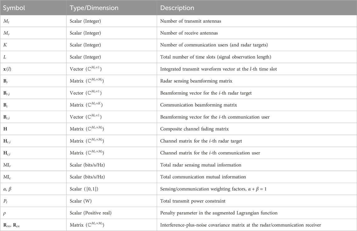
Table 1. Notation.
2 System model and problem formulation
2.1 Time-division signal model
As shown in Figure 1, we considered the DFRC system equipped with
where
where
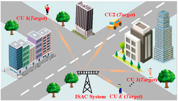
Figure 1. The ISAC system model.
Note that
where
Next, we will introduce the system model of radar sensing and communication transmission in detail.
2.1.1 Radar sensing model
The echo of the dual-function signal transmitted by the base station (BS) reflected by the target at the
Note that
where
We calculate the covariance of system interference plus noise, which can be expressed as
Thus, the probability density of system interference plus noise
Toward this end, the differential entropy corresponding to system interference plus noise
The probability density function (PDF) of the system detecting targets can be expressed as
Furthermore, its corresponding differential entropy can be formulated as
In summary, the system detection of MI is given by
The system total MI of the radar detection can be expressed as
We will introduce the system communication MI next.
2.1.2 Communication transmission model
When the system communicates with the communication users, the system signal received at the
where
Note that
Furthermore, the interference-plus-noise variance matrix is expressed as
Thus, the PDF of the system interference plus noise can be represented as
Therefore, the communication interference plus noise corresponding differential entropy can be formulated as
Similarly, the system communication user PDF is given by
To this end, the corresponding differential entropy can be expressed as
Hence, the MI of the
The system total MI of the communication users can be represented as
2.1.3 Optimization problem formulation
In the DFRC system, we comprehensively consider the detection and communication performance of the system through MI. Therefore, when constructing the system optimization problems, it is essential to address the influence of radar and communication MI simultaneously. The system optimization problem objective function can be formulated as follows:
where
Thus, the system optimization problem can be represented as follows:
When we substitute Equations 15, 25 into Equation 28, the system optimization problem can be expressed as
Due to the typical concave form of the
2.2 General signal model
2.2.1 System model
In the general signal model, we assumed that the communication user and detection target are the same object in this system, without losing generality. In that case, the system signal model can be recast as
where
For convenience, the interference-plus-noise signal can be represented as
Note that
Thus, the PDF of the system interference plus noise can be represented as
Therefore, the communication interference plus the noise corresponding differential entropy can be formulated as
Similarly, the system communication user PDF is given by
Hence, it corresponds to the differential entropy, which can be expressed as
2.2.2 Optimization problem formulation
In the DFRC system, we comprehensively consider the detection and communication performance through MI. Thus, when we construct the system optimization problems, it is essential to trade off the effect on radar and communication MI simultaneously. Therefore, the system objective function in the optimization problem and the MI of the system can be formulated as follows:
It is a necessary prerequisite for the system to satisfy the basic power requirements, so the system’s power constraints can be expressed as
To this end, the optimization problem can be represented as follows:
In the following section, we will discuss and analyze the solution of the optimization problem in detail.
3 System optimization problem solving
3.1 Time-division model optimization
Due to the radar and communication beamforming matrix
For convenience, let
where
Actually, when the system detects the target, the remaining users are considered interference, and when the system communicates with the user, the remaining targets are also considered interference in this model. Therefore, the system detection, interference, and communication covariance matrix can be represented as
3.1.1 Communication beamforming matrix update
The system communication beamforming matrix is determined for each
Similarly, the differential of Equation 25 with respect to
In summary, by combining the partial derivatives of the communication covariance matrix (Equation 44) and the detection covariance matrix (Equation 45), the gradient of the augmented Lagrangian function with respect to
3.1.2 Radar beamforming matrix update
Similarly, for each
Similarly, the differential of Equation 25 at approximately
The gradient of Equation 42 regarding
The corresponding gradient is obtained after the above derivation. This model utilizes the dual variable sub-gradient descent idea, uses the Lagrange multiplier algorithm to construct the corresponding gradient function, and then iteratively updates it to obtain the corresponding optimization solution. See the Supplementary Appendix for the detailed concavity proof.
Through the above analysis, the system optimization solution can be obtained by using the augmented Lagrangian multiplier method. However, the selection of penalty parameter
However, it is difficult to simultaneously satisfy the optimal performance of sensing and communication in reality. Therefore, it is necessary to comprehensively consider the trade-off between system sensing and communication performance and introduce two parameter factors
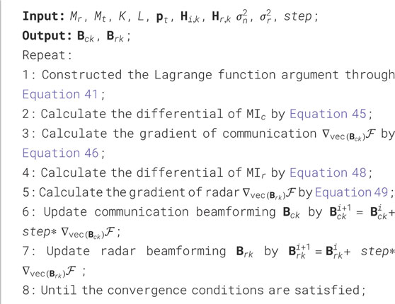
Algorithm 1. JOINT optimization algorithm for solving Equation 30.
Another form of signal besides time-division multiplexing, which directly treats the system signal as an integrated signal, was considered. The optimization process under this model will be explained in detail in the next subsection.
3.2 General model optimization
It is difficult to solve the system problem due to the non-convexity of the objective function in the optimization problem (Equation 40). Therefore, utilizing the equivalent function to replace the objective function is considered, and the classic Minorization–Maximization (MM) algorithms to design waveforms are applied. Next, we will briefly introduce the basic principles of MM, which can be divided into a minorization step and a maximization step.
Minorization step: find a surrogate function
where
Maximization step: To solve the maximization problem
Because
First, to make the expression of the formula more compact, let
in Equation 52
3.2.1 A quadratic function of B
The MM algorithm must find its surrogate function, which can be approximated by its function margin. In order to facilitate processing, it is first equivalently transformed into the following form. The relevant detailed proof can be found in Naghsh et al. (2017).
where
In addition, the objective function (Equation 53) can be equivalently transformed into
where
The gradient of the
In the meantime, transforming
Consequently, as
After the First-order Taylor expansion processing, the first and second terms on the right side of the equation in the original objective function are constant terms, and we neglect the constant terms. At this point, the original optimization problem can be equivalently recast as
Due to
For the convenience of representation, we let
The objective function of the optimization problem can be reformulated as
where
3.2.2 A logdet of the linear function of B
The essence of the MM algorithm is to find a replacement function that is equivalent to the original optimization objective function. Therefore, the form of equivalent replacement is not limited to one form. In the previous section, we discussed a quadratic function form of the replacement function. At the same time, considering the characteristics of the optimization objective function itself, we further analyze the linear form of the logarithmic determinant of the replacement function. Because
where
Note that from the properties of the logarithmic determinant, it can be inferred that when the independent variable function is positive semidefinite, that is,
Hence, the objective function surrogate function can be expressed as follows:
The system optimization problem can be equivalently reformulated as
It is obvious that the processed optimization problem has a typical convex optimization solution form that is easier to solve and can be directly obtained using a numerical toolbox. This value is still the global optimal solution.
3.2.3 The MM convergence analysis
To demonstrate the performance of the MM algorithm, the convergence of the alternative function is discussed here, as the influence of iteration is taken into account in the system optimization solution.
It can be clearly seen from the above equation that as the number of iterations
The algorithm flow is illustrated in the Algorithms 2 to provide an intuitive understanding of the solution process for the joint optimization problem. The effectiveness of the proposed method and scheme will be analyzed and discussed in the following section.
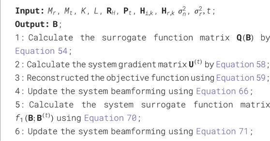
Algorithm 2. MM algorithm for solving Equation 40.
To complement the convergence analysis discussed previously, we now present a comprehensive evaluation of the computational complexity. A comparative analysis of the proposed JOINT and MM algorithms against classical water-filling, WMMSE, and Successive Convex Approximation (SCA) algorithms is performed, with the key results presented in the Table 2.
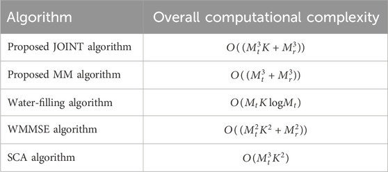
Table 2. Comparison of algorithm computational complexity.
4 Numerical simulation
In this section, the proposed algorithm is verified by simulation, and the numerical experiment parameters are set. For the convenience of analysis and understanding, consider two communication users for communication without loss of generality. The total system power budget is 20 W. It is assumed that the communication channel and radar channel obey the complex Gaussian distribution, with variances of
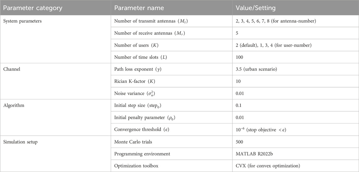
Table 3. Simulation parameter configuration.
The beamforming matrix
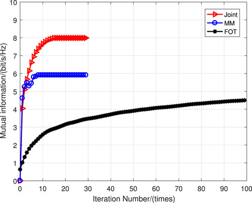
Figure 2. Analysis of the iterative convergence of the optimization algorithms.
From the simulation results, it can be clearly seen that the joint optimization algorithm and the MM algorithm can converge in fewer iterations, while the First-order Taylor (FOT) expansion method requires more iterations to complete convergence. In addition, the system performance of the joint optimization is better than that of the MM algorithm and the FOT expansion algorithm. The reason for this is that in the two different optimization modes of the system, both the MM algorithm and the FOT expansion approximate the system optimization problem, which results in performance degradation.
There are certain shortcomings in analyzing the superiority of various methods solely based on the convergence of system algorithms. In the system optimization process, changes in system power can have a significant impact on the performance of various aspects of the system. As an important indicator in the ISAC system, the variation of system power will directly affect system performance. Therefore, based on this, we will consider the impact of system power variation on system performance, and comprehensively analyze the specific performance of the classic water injection algorithm and the MM, FOT, and JOINT methods mentioned in the article with the variation of system power. Further analysis of the changes in system power with the increase of power is shown in the simulation results in Figure 3.
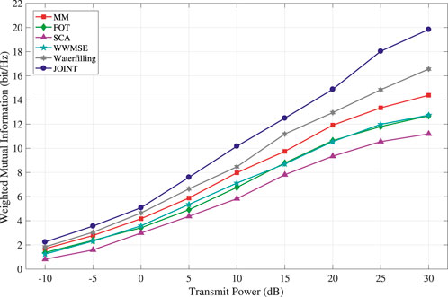
Figure 3. System optimization of MI vs. the system power.
From the graph, it can be seen that as the system transmission power increases, the system MI gradually increases. In the simulation comparison, we use the typical water injection power allocation algorithm as the benchmark algorithm. The graph shows that the joint optimization has the best effect, followed by the MM algorithm, and the FOT expansion has the worst effect. The performance of the water injection algorithm is between the MM algorithm and the FOT expansion method, which further confirms that the joint optimization has the best effect. Similarly, due to the approximate scaling of the MM and FOT expansion methods in solving system optimization problems, both have a certain performance loss. However, compared to the FOT expansion, the MM algorithm still has better performance, indicating that MM can better solve optimization problems in the approximation process than the FOT expansion. Due to the discussion of two different scenarios of time-division signal and general signal models during system modeling, which have different requirements for system communication users, further analysis was conducted on the impact of different numbers of users on system MI performance. The simulation results are shown in Figure 4.
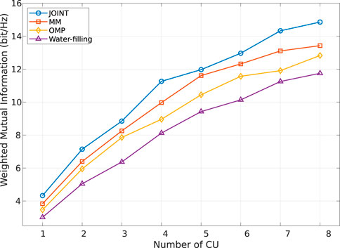
Figure 4. System optimization of MI vs. the system communication users.
As can be seen from Figure 4, as the number of communication users increases, the system weighted MI increases accordingly, showing an overall increasing trend. Due to the correlation between the system MI and the number of communication users during the communication transmission process, the system MI naturally shows an increasing trend as the number of system users increases. In addition, the system MI under various optimization methods always shows the best joint optimization effect, followed by MM, and the FOT expansion is the worst. The water injection algorithm is between MM and the FOT expansion. The reason for this is similar to the performance mentioned above, both of which are due to the approximation involved in the processing of MM and the FOT expansion. In addition to the change in the number of communication users, the number of transmitting antennas also affects the power allocation of the system. Therefore, the simulation results of the system performance changing with the number of antennas are shown in Figure 5.
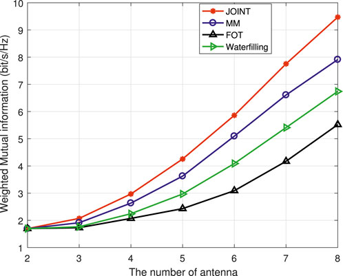
Figure 5. System optimization of MI vs. the number of antennas.
From the simulation picture, it can be seen that as the number of antennas increases, the system MI also gradually increases. Although the overall performance of the system also maintains the best JOINT performance, the FOT expansion is the worst, and it is the same with the trend of increasing the number of communication users. When the number of communication users in the system increases, several optimization algorithms show a significant increase. When the number of antennas in the system changes, the change in system MI is relatively gentle when the number of antennas is small. When the number of antennas is large, the increase in MI is more obvious. This further indicates that both the number of communication users and antennas in the system will affect system MI, but the impact of communication users is more obvious.
Due to the significant influence of weight factors in the process of system performance balancing optimization, in order to further analyze the impact of weight factors on system perception and communication performance, the system perception MI, communication MI, and jointly optimized MI that vary with weight factors are discussed and analyzed. In the aforementioned analysis, it is mentioned that weight factors must be adjusted according to the dynamic changes in system performance. Based on continuous changes in weight factors, relevant simulation results are obtained, and the simulation effect is shown in Figure 6.
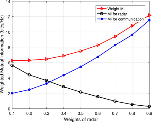
Figure 6. System optimization of the weight of MI vs. the system weight factor.
Based on the above analysis, only the joint optimization of the system was discussed in the weight factor analysis. The simulation results show that as the weight factor increases, the performance of the system’s sensing and communication varies. The radar performance shows a decreasing trend with the increase of the weight factor, while the communication MI increases with the increase of system weight. On the other hand, the system weighted MI generally shows an upward trend, which also indicates that the system sensing and communication performance can achieve relative balance with the change of the system weight factor. The overall trend of change also satisfies the law of system performance changes, once again proving the effectiveness of the algorithm.
5 Conclusion
This article investigates two distinct ISAC signal frameworks, unified under a mutual information (MI) performance metric. To solve the resulting optimization problems, a dual sub-gradient ascent method and a Minorization–Maximization (MM) algorithm are developed. The use of MI from information theory offers a more general and fundamental approach to system optimization than direct SINR-based modeling. The proposed signal model incorporates not only sensing-oriented waveform design but also time-division structural characteristics, providing an integrated system representation. Simulation results demonstrate that the proposed framework achieves strong overall performance and effectively balances sensing and communication capabilities. Future work will focus on advanced co-design methodologies for sensing-communication performance trade-offs.
Data availability statement
The original contributions presented in the study are included in the article/Supplementary Material; further inquiries can be directed to the corresponding author.
Author contributions
ZP: Conceptualization, Investigation, Writing – original draft. FC: Methodology, Validation, Writing – review and editing.
Funding
The author(s) declare that financial support was received for the research and/or publication of this article. This work is supported by the National Natural Science Foundation of China (62301053).
Acknowledgements
The successful completion of this manuscript is due to support from the projects of the National Natural Science Foundation of China and the School of Information Engineering, Chongqing Jiaotong University, as well as the many constructive comments put forward by the reviewers of this article.
Conflict of interest
The authors declare that the research was conducted in the absence of any commercial or financial relationships that could be construed as a potential conflict of interest.
Generative AI statement
The author(s) declare that no Generative AI was used in the creation of this manuscript.
Any alternative text (alt text) provided alongside figures in this article has been generated by Frontiers with the support of artificial intelligence and reasonable efforts have been made to ensure accuracy, including review by the authors wherever possible. If you identify any issues, please contact us.
Publisher’s note
All claims expressed in this article are solely those of the authors and do not necessarily represent those of their affiliated organizations, or those of the publisher, the editors and the reviewers. Any product that may be evaluated in this article, or claim that may be made by its manufacturer, is not guaranteed or endorsed by the publisher.
Supplementary material
The Supplementary Material for this article can be found online at: https://www.frontiersin.org/articles/10.3389/frsip.2025.1700979/full#supplementary-material
References
Bazzi, A., and Chafii, M. (2023). On integrated sensing and communication waveforms with tunable papr. IEEE Trans. Wirel. Commun. 22, 7345–7360. doi:10.1109/twc.2023.3250263
Bazzi, A., and Chafii, M. (2025). Mutual information based pilot design for isac. IEEE Trans. Wirel. Commun. 73, 7914–7930. doi:10.1109/tcomm.2025.3545658
Bica, M., Huang, K.-W., Koivunen, V., and Mitra, U. (2016). Mutual information based radar waveform design for joint radar and cellular communication systems. 2016 IEEE Int. Conf. Acoust. Speech Signal Process. (ICASSP), 3671–3675. doi:10.1109/ICASSP.2016.7472362
Chen, X., Yang, Q., Deng, B., and Wang, H. (2020). Robust interference waveform design in fuzzy colored noise based on mutual information. J. Appl. Remote. Sens. 14, 1–016516. doi:10.1117/1.jrs.14.016516
Chen, L., Wang, Z., Du, Y., Chen, Y., and Yu, F. R. (2022). Generalized transceiver beamforming for dfrc with mimo radar and mu-mimo communication. IEEE J. Sel. Areas Commun. 40, 1795–1808. doi:10.1109/jsac.2022.3155515
Cui, Y., Koivunen, V., and Jing, X. (2020). Mutual information based co-design for coexisting mimo radar and communication systems. 2020 IEEE Int. Conf. Commun. Work. ICC Work., 1–6. doi:10.1109/iccworkshops49005.2020.9145384
Dong, F., Liu, F., Lu, S., Yuan, W., Cui, Y., Xiong, Y., et al. (2023). Waveform design for communication-assisted sensing in 6g perceptive networks. 2023 IEEE/CIC Int. Conf. Commun. China (ICCC), 1–6. doi:10.1109/ICCC57788.2023.10233679
Gao, S., Cheng, X., and Yang, L. (2021). Mutual information maximizing wideband multi-user (wmu) mmwave massive mimo. IEEE Trans. Commun. 69, 3067–3078. doi:10.1109/tcomm.2021.3053967
He, J., Chen, L., and Wei, G. (2021). Waveform design for dual-functional radar and communication design based on conditional mi. 2021 7th Int. Conf. Comput. Commun. (ICCC), 1026–1030. doi:10.1109/iccc54389.2021.9674284
Huang, K., Bică, M., Mitra, U., and Koivunen, V. (2015). Radar waveform design in spectrum sharing environment: coexistence and cognition. 2015 IEEE Radar Conf. (RadarCon), 1698–1703. doi:10.1109/radar.2015.7131272
Liu, Y., Liao, G., Xu, J., Yang, Z., and Zhang, Y. (2017). Adaptive ofdm integrated radar and communications waveform design based on information theory. IEEE Commun. Lett. 21, 2174–2177. doi:10.1109/lcomm.2017.2723890
Liu, F., Masouros, C., Li, A., Ratnarajah, T., and Zhou, J. (2018). Mimo radar and cellular coexistence: a power-efficient approach enabled by interference exploitation. IEEE Trans. Signal Process 66, 3681–3695. doi:10.1109/tsp.2018.2833813
Liu, Y., Liao, G., and Yang, Z. (2019). Robust ofdm integrated radar and communications waveform design based on information theory. Signal Process. 162, 317–329. doi:10.1016/j.sigpro.2019.05.001
Liu, X., Huang, T., Shlezinger, N., Liu, Y., Zhou, J., and Eldar, Y. C. (2020). Joint transmit beamforming for multiuser mimo communications and mimo radar. IEEE Trans. Signal Process 68, 3929–3944. doi:10.1109/tsp.2020.3004739
Liu, F., Zheng, L., Cui, Y., Masouros, C., Petropulu, A. P., Griffiths, H., et al. (2023). Seventy years of radar and communications: the road from separation to integration. IEEE Signal Process Mag. 40, 106–121. doi:10.1109/msp.2023.3272881
Naghsh, M. M., Modarres-Hashemi, M., Kerahroodi, M. A., and Alian, E. H. M. (2017). An information theoretic approach to robust constrained code design for mimo radars. IEEE Trans. Signal Process 65, 3647–3661. doi:10.1109/tsp.2017.2692747
Qian, J., Lu, M., and Huang, N. (2020). Radar and communication co-existence design based on mutual information optimization. IEEE Trans. Circuits Syst. II Express Briefs 67, 3577–3581. doi:10.1109/tcsii.2020.2998801
Qian, J., Zhao, L., Shi, X., Fu, N., and Wang, S. (2022). Cooperative design for mimo radar-communication spectral sharing system based on mutual information optimization. IEEE Sensors J. 22, 17184–17193. doi:10.1109/jsen.2022.3192348
Shi, Q., Razaviyayn, M., Luo, Z., and He, C. (2011). An iteratively weighted mmse approach to distributed sum-utility maximization for a mimo interfering broadcast channel. IEEE Trans. Signal Process. 59, 4331–4340. doi:10.1109/tsp.2011.2147784
Sun, G., He, Z., Tong, J., Yu, X., and Shi, S. (2021). Mutual information-based waveform design for mimo radar space-time adaptive processing. IEEE Trans. Geosci. Remote Sens. 59, 2909–2921. doi:10.1109/tgrs.2020.3008320
Tang, B., and Li, J. (2019). Spectrally constrained mimo radar waveform design based on mutual information. IEEE Trans. Geosci. Remote Sens. 67, 821–834. doi:10.1109/tsp.2018.2887186
Tian, T., Zhang, T., Kong, L., Cui, G., and Wang, Y. (2019). Mutual information based partial band coexistence for joint radar and communication system. 2019 IEEE Radar Conf. (RadarConf), 1–5. doi:10.1109/radar.2019.8835671
Yang, Y., and Blum, R. S. (2007). Mimo radar waveform design based on mutual information and minimum mean-square error estimation. IEEE Trans. Aerosp. Electron Syst. 43, 330–343. doi:10.1109/taes.2007.357137
Yuan, X., Feng, Z., Zhang, J. A., Ni, W., Liu, R. P., Wei, Z., et al. (2021). Spatio-temporal power optimization for mimo joint communication and radio sensing systems with training overhead. IEEE Trans. Veh. Technol. 70, 514–528. doi:10.1109/tvt.2020.3046438
Zhang, Z., Du, Z., and Yu, W. (2020). Mutual-information-based ofdm waveform design for integrated radar-communication system in gaussian mixture clutter. IEEE Sensors Lett. 4, 1–4. doi:10.1109/lsens.2019.2946735
Zhang, A., Rahman, M. L., Huang, X., Guo, Y. J., Chen, S., and Heath, R. W. (2021a). Perceptive mobile networks: cellular networks with radio vision via joint communication and radar sensing. IEEE Veh. 16, 20–30. doi:10.1109/mvt.2020.3037430
Keywords: integrated sensing and communication, mutual information, beamforming, adaptive weight, optimization
Citation: Pu Z and Chen F (2025) MI-based beamforming optimization framework for integrated sensing and communication. Front. Signal Process. 5:1700979. doi: 10.3389/frsip.2025.1700979
Received: 08 September 2025; Accepted: 07 October 2025;
Published: 12 November 2025.
Edited by:
Le Liang, Southeast University, ChinaReviewed by:
Ahmad Bazzi, New York University Abu Dhabi, United Arab EmiratesNur Alamsyah, Universitas Informatika dan Bisnis Indonesia, Indonesia
Copyright © 2025 Pu and Chen. This is an open-access article distributed under the terms of the Creative Commons Attribution License (CC BY). The use, distribution or reproduction in other forums is permitted, provided the original author(s) and the copyright owner(s) are credited and that the original publication in this journal is cited, in accordance with accepted academic practice. No use, distribution or reproduction is permitted which does not comply with these terms.
*Correspondence: Zhiwei Pu, cHV6aGl3ZWlAY3FqdHUuZWR1LmNu