1
Department of Experimental Psychology, Otto-von-Guericke-University Magdeburg, Magdeburg, Germany
2
Department of Cognitive Neurology, Max Planck Institute for Human Cognitive and Brain Sciences, Leipzig, Germany
Objects in our visual environment are arranged in depth and hence there is a considerable amount of overlap and occlusion in the image they generate on the retina. In order to properly segment the image into figure and background, boundary interpolation is required even across large distances. Here we study the cortical mechanisms involved in collinear contour interpolation using fMRI. Human observers were asked to discriminate the curvature of interpolated boundaries in Kanizsa figures and in control configurations, which contained identical physical information but did not generated subjective shapes. We measured a spatially precise spin-echo BOLD signal and found stronger responses to subjective shapes than non-shapes at the subjective boundary locations, but not at the inducer locations. The responses to subjective contours within primary visual cortex were retinotopically specific and analogous to that to real contours, which is intriguing given that subjective and luminance-defined contours are physically fundamentally different. We suggest that in the absence of retinal stimulation, the observed activation changes in primary visual cortex are driven by intracortical interactions and feedback, which are revealed in the absence of a physical stimulus.
Objects are often partially occluded by other objects and still perceived as coherent entities. It is still an unanswered question how the visual system assigns different image parts to figure and background. A well-known instance of boundary completion is taking place in the Kanizsa figure, in which a number of inducing elements, discs with a particular opening, are geometrically aligned such that an occluding surface is perceived on top of solid circles (Kanizsa, 1976
; Figure 1
). Due to proper geometrical alignment of the local inducers subjective boundaries are perceived as a collinear extension of the inducers. The contours are called subjective or illusory contours (IC) because there is no corresponding change in the physical stimulus intensity (e.g., luminance or texture) at the location of the apparent boundary. Hence subjective shapes provide us with the unique opportunity to study the cortical mechanisms that generate a contour percept in the absence of the distal stimulus.
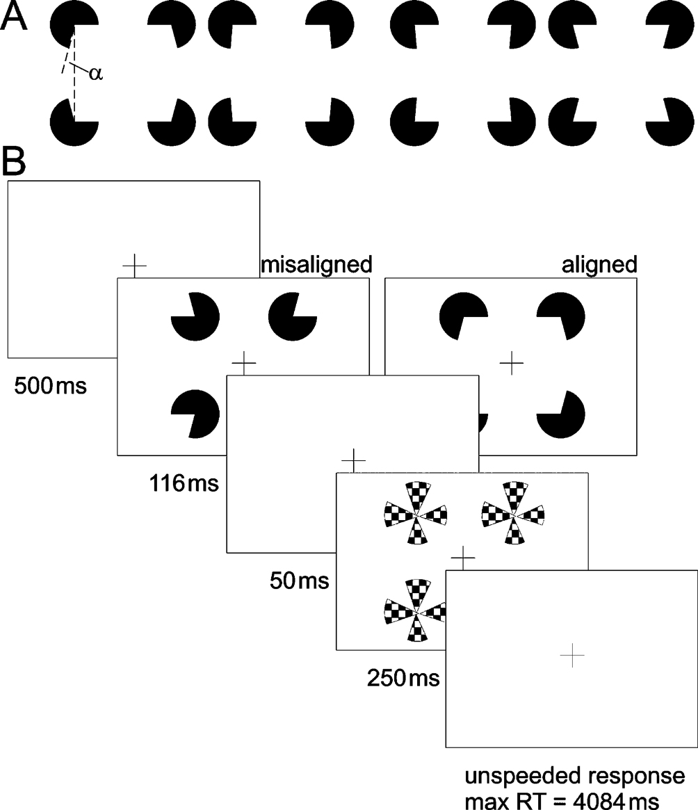
Figure 1. Experimental stimuli and trial. (A) Kanizsa stimuli consisted of four inducers (note that stimulus depictions in the manuscript are contrast reversed), with openings (alpha) varying between ±15 around 90°. Openings larger than 90° resulted in convex shapes (two left-hand figures) and those smaller than 90° in concave shapes (two right hand figures). The ease of curvature discrimination depended on the magnitude of alpha. Large values resulted in pronounced curvature (outermost stimuli), whereas curvature was hardly detectable for small alpha, (innermost stimuli). (B) Participants performed the task inside the scanner. They were required to fixate the central cross during the entire experiment. Inducers (aligned or misaligned) were presented for 100 ms followed by a 250 ms presentation of a mask stimulus after an intervening blank period of 50 ms. Participants were required to discriminate between convex and concave shapes by pressing the right or left response button, respectively, within the remaining inter trial interval of 4084 ms. Auditory feedback (1000 Hz tone of 300 ms duration) followed each correct response.
Electrophysiological studies in non-human primates have shown that neurons in early visual cortex (V1/V2) respond to subjective contours (Grosof et al., 1993
; Lee and Nguyen, 2001
; Peterhans and von der Heydt, 1989
; Ramsden et al., 2001
; Sheth et al., 1996
; Sugita, 1999
). Some of the functional imaging studies with human subjects reported IC-sensitivity predominantly in higher visual areas (Hirsch et al., 1995
; Mendola et al., 1999
; Murray et al., 2002
; Ritzl et al., 2003
; Stanley and Rubin, 2003
) like the Lateral Occipital Complex (LOC), which has been shown to respond preferentially to increasingly complex, object-like stimuli (see Grill-Spector and Malach, 2004
; Grill-Spector et al., 2001
for review). Other studies reported IC-related activity also in earlier extrastriate areas (Ffytche and Zeki, 1996
; Hirsch et al., 1995
; Larsson et al., 1999
; Ritzl et al., 2003
) or even in primary visual cortex (Maertens and Pollmann, 2005
; Montaser-Kouhsari et al., 2007
; Seghier et al., 2000
). Using functional magnetic resonance imaging (fMRI), Montaser-Kouhsari et al. (2007)
observed neural adaptation to illusory contours in abutting gratings in most of the visual areas. Seghier et al. (2000)
reported fMRI BOLD changes in response to moving Kanizsa-type subjective contours. We compared pre- vs. post-learning BOLD responses to Kanizsa-type subjective contours in a perceptual learning task (Maertens and Pollmann, 2005
) and observed significant learning related changes in V1. Furthermore, we showed that in the absence of the analogous V1 representation, which can be simulated under monocular viewing conditions in the ‘blind spot’ region in V1, curvature discrimination with subjective figures is severely impaired (Maertens and Pollmann, 2007
).
In the present experiment, we wanted to study whether responses to subjective contours in V1 do indeed follow the retinotopic representational pattern of real contours. In our earlier learning experiment (Maertens and Pollmann, 2005
) we compared BOLD responses to subjective contours before and after training. In the current experiment we introduce a control configuration which is almost identical to the Kanizsa shape except that it does not contain a subjective shape and subjective boundaries because the inducers’ mouths are rotated outwards. We randomly intermixed Kanizsa and control stimuli in order to probe spatially specific for subjective contour evoked responses. We adopted a curvature discrimination paradigm which – in order to yield accurate performance – requires a spatially precise representation of the subjective contour (Ringach and Shapley, 1996
).
We reasoned that in order to detect slight differences in subjective contour curvature, the subjective contour should be represented by neural populations that provide the appropriate spatial resolution (e.g., small receptive field size, retinotopic organization, orientation selectivity). The reasoning follows the psycho-anatomic matching logic (Julesz, 1971, cf. Hochstein and Ahissar, 2002
), that different degrees of performance accuracy may be indicative of different cortical processing levels. Since primary visual cortex has the most precise retinotopy and the smallest average receptive field sizes, we reasoned that the disambiguation of slight differences in subjective contour curvature would heavily rely on a neural representation of the subjective contour in V1.
Going beyond previous work, we investigated the retinotopic specificity of subjective contour-related BOLD changes in V1. In contrast to Montaser-Kouhsari et al. (2007)
we used collinear Kanizsa-type subjective contours to ensure that BOLD responses to inducers and subjective stimulus parts are spatially separable. We performed a localizer scan in order to determine the putative locations of subjective contours and inducers within primary visual cortex. We hypothesized that if subjective contours are represented retinotopically within V1, then Kanizsa stimuli should elicit stronger responses than control stimuli at the putative contour locations. As a control we compared BOLD responses to Kanizsa and control stimuli at the inducer locations, because they should be identical. We also varied the center-to-center distance between inducers of constant size, as it has been shown that subjective ratings of contour clarity (Kellman and Shipley, 1992
) as well as performance-based measures increase with increasing contour support (Ringach and Shapley, 1996
). We therefore predicted that if the perception of contour clarity depends on the representation of the subjective contour in V1, then the BOLD response will become stronger with increasing contour support.
In order to obtain sufficient spatial specificity of the functional MRI signal we applied a spin-echo echo-planar-imaging-sequence (SE-EPI) at a magnetic field strength of 3 Tesla. In spin-echo compared to the more common gradient-echo (GE) EPI experiments, the spin dephasing due to T2* effects is refocused, so that at the time of signal readout (time-to-echo, TE) the only loss in transverse magnetization is due to T2. Spin echo imaging is therefore insensitive to susceptibility artifacts, which are caused by magnetic field inhomogeneities (Jezzard et al., 2001
). Of even greater importance for the present study was that the SE-BOLD signal is predominantly sensitive to extravascular water surrounding capillaries, in addition to being sensitive to intravascular water spins in vessels of all sizes. Using flow-compensating diffusion-weighting at 3T the former can be effectively reduced leaving exclusively signal contributions from the capillaries (Jochimsen et al., 2004
; Norris et al., 2002
). In this way, we attained the high spatial specificity necessary to demonstrate spatially specific activation changes in response to illusory contours within the primary visual cortex. The high spatial specificity of SE-EPI comes at the cost of a reduced overall functional sensitivity. We counteracted this sensitivity loss by the use of a phased array coil, which has an improved sensitivity compared with a volume (head) coil.
Participants
Fourteen observers were paid for their participation in one 60 minutes scanning session. Half of them were female. Their mean age was 25 years (SD = 2.5). All participants were right-handed and had normal or corrected-to-normal vision. Participants gave their informed written consent according to the guidelines of the Max-Planck-Institute.
Stimuli and Design
Stimuli were presented at a resolution of 800 × 600 pixels on a 16" back-projection screen, mounted in the bore of the magnet behind the participant’s head, using a liquid crystal display (LCD) projector. Participants viewed the screen by wearing mirrored glasses. Four white inducers were presented tachistoscopically on a black background. Inducers varied in the magnitude of their openings in order to create convex (‘fat’) and concave (‘thin’) shapes. We used openings (α) which were either larger or smaller than 90° (75 < α < 105), and which had to be classified as ‘fat’ or ‘thin’, accordingly (Figure 1
A). Inducers of constant size were presented at two different peripheral eccentricities (see below). Their diameter was 3.5 cm corresponding to 2.4° visual angle. Four white pinwheel masks, consisting of four wedges of 45° each, were presented at the inducer positions to limit their effective viewing time (Figure 1
B).
Stimulus delivery and response registration were controlled by Presentation® software (Version 9.51, http://nbs.neuro-bs.com). A trial started with a 500 ms fixation period, followed by stimulus presentation for 116 ms. After a blank period of 50 ms a mask was presented for 250 ms (Figure 1
B). No time limit was imposed on participants’ response. They indicated whether they had perceived a concave or convex shape by pressing either the left or the right button of a two-button response pad, with their index or middle finger, respectively. Trial duration was fixed at five seconds. Observers were instructed to maintain fixation during the scans, and due to the rapid presentation voluntary eye movements are highly unlikely. Kanizsa and control stimuli were constructed from inducers that either were aligned to form an illusory square, e.g., their openings were facing inwards, or they were misaligned, e.g., their openings were facing to the margins of the screen. Stimuli did also vary with respect to the distance between the inducers. The center-to-center distance between the inducers was 7.4°, in the near, or 11.2° visual angle, in the far condition, yielding support ratios of 0.32 and 0.21, respectively. The support ratio (SR) describes the ratio between the luminance-defined part of the illusory contour and its total side length.
Procedure
All participants performed a training block consisting of twenty trials with the experimental stimuli outside the scanner. The training block was repeated until at least 15 out of 20 trials were answered correctly. During scanning, participants’ curvature discrimination thresholds were measured, using a weighted up-down method for two response alternatives (Kaernbach, 1991
). The starting inducer angle (alpha) was randomly set to the maximum deviation of either + or –15°. Each wrong response entailed an increment of 6° to make the deviation from 90° more pronounced. After the first three reversals the step size was decreased to 3°. Each correct response was followed by a reduction in the angular deviation from 90° by an amount of 2°. Again, after the first three reversals this step size was reduced to 1°. The staircase converged on a 75% correct response level. Two functional scanning blocks were performed each involving a quadruple staircase procedure (one for each combination of inducer distance and orientation), that was terminated after 25 trials of each condition. In addition, ten baseline 8 trials (null-events) were interspersed within the resulting 100 experimental trials, in which only the fixation cross was presented for five seconds without any response requirements.
fMRI Methods
Magnetic resonance (MR) imaging was performed on a 3T Siemens Magnetom Trio scanner using an eight-channel phased-array head coil. First, a T1-weighted anatomical scan was recorded with a modified driven equilibrium Fourier transform (MDEFT) sequence (Norris, 2000
). Twelve axial slices were recorded which were aligned in parallel to the calcarine sulcus, to cover the visual cortex. The sequence parameters were as follows: TR = 1300 ms, TI = 650 ms, TE = 7.4 ms, slice-thickness = 2 mm, slice-gap = 0.4 mm, FOV = 128 mm × 128 mm with an in-plane resolution of 2 mm × 2 mm. Oversampling in the phase-encoding direction was applied to achieve the desired in-plane resolution (‘zoom-EPI’) and to remove any fold-in signal from outside the FOV. The functional part of the session consisted of three spin-echo EPI scans (TR = 2 seconds, TE = 85 ms, bandwidth = 1346 Hz/Px, matrix 64 × 64, phaseoversampling).
The functional slices were aligned as in the anatomical scan using the same FOV, slice-thickness and slice-gap. Two experimental functional scans with 310 repetitions were performed using the experimental paradigm as described above, as well as one functional localizer scan containing 318 repetitions (see below).
Statistical analysis was carried out using FEAT (FMRI Expert Analysis Tool) Version 5.63, part of FSL (FMRIB’s Software Library, www.fmrib.ox.ac.uk/fsl). Movement artifacts were corrected using MCFLIRT (Jenkinson et al., 2002
). Differences in slice acquisition time were corrected using Fourier-space time-series phase-shifting. Potential baseline signal drifts were removed applying a high pass temporal filter (Gaussian-weighted least-squares straight line fitting, with sigma = 50.0 seconds). In the spatial domain data were smoothed using a Gaussian kernel with a full width at half maximum (FWHM) of 4 mm. All volumes were mean-based intensity normalized by the same factor. Time-series statistical analysis was carried out using FILM (Woolrich et al., 2001
). For the localizer scan z (Gaussianized T/F) statistic images were thresholded using clusters determined by z > 2.3 and a corrected cluster significance threshold of p = 0.05 (Worsley et al., 1992
).
In order to determine regions of interest, the functional data from the localizer scan were individually registered onto their corresponding high resolution anatomical data (1 × 1 × 1 mm) using FLIRT (Jenkinson and Smith, 2001
): (i) the functional slices were geometrically aligned with the 2D MDEFT images using a rigid body transformation with 3 parameters, (ii) the 2D MDEFT slices were aligned with the 3D anatomy using a rigid, linear transformation with three translational and three rotational parameters, (iii) the resulting transformation matrices were concatenated using ConvertXfM (FLIRT), and finally the output matrix was applied to the functional data.
Stimulus Localizer, Retinotopy and Flattening
The purpose of the localizer was (a) to map the cortical sites responsive to illusory contours and inducers at the two stimulus eccentricities employed in the main experiment, and (b) to determine the border between visual areas V1 and V2. All stimuli were black-and-white checkerboard patterns presented on a black background that reversed contrast at a rate of 8 Hz. The inducer localizer was composed of four circles that had a diameter of 2.4° visual angle (equivalent to that of the inducers) and their centers were aligned with the center positions of the inducers in the main experiment for both, the near and far conditions. In the contour localizer four checkered bars (0.6° wide and 5° or 8.5° long), aligned as to form a square with missing edges, were presented at 3.7° or 5.5° from fixation in order to stimulate the putative illusory contour representations in the near and far condition, respectively, complementary to the inducer positions. In addition, we mapped the horizontal (HM) and vertical meridians (VM) using alternating ‘hourglass’ and ‘bow tie’ shaped checkerboard patterns that were perspectively scaled to account for cortical magnification. Circles and bars, as well as the meridian mapping stimuli were presented for eight seconds each, followed by an eight seconds fixation baseline. One full cycle thus lasted 96 seconds and might have consisted of the following sequence: near circles – far contours – horizontal meridian – vertical meridian – near contours – far circles. A run was composed of 6 1/2 cycles whereby data from the first 1/2 cycle were discarded to avoid magnetic saturation effects, and a break of 30 seconds was introduced between the third and the fourth cycle. Periods of stimulation were contrasted with fixation periods to demarcate occipital visual area V1 (Engel et al., 1997
; Sereno et al., 1995
), and to localize the stimulus positions (Figure 2
). Brain inflation was performed following standard procedures as implemented in the Computerized Anatomical Reconstruction and Editing Toolkit (Caret, Van Essen et al., 2001
; http://brainmap.wustl.edu/caret).
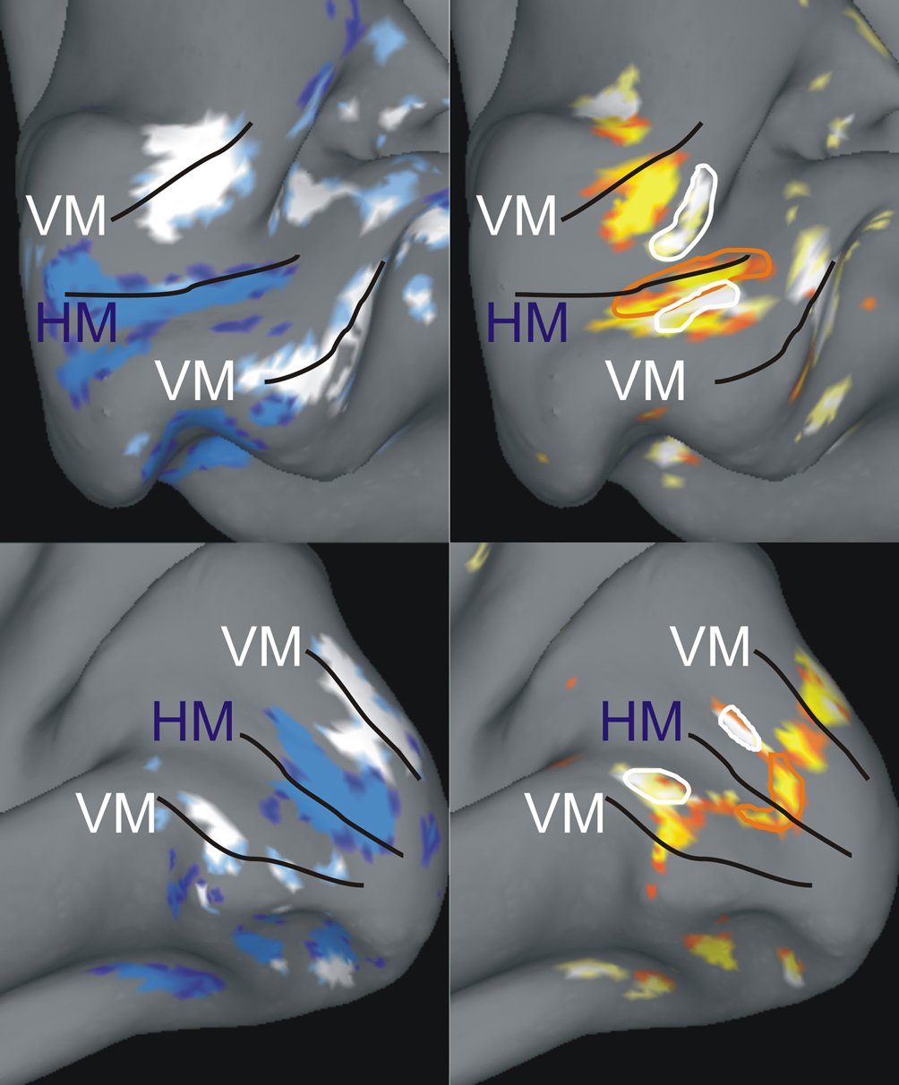
Figure 2. Examples of individual z-maps projected onto inflated anatomical surfaces. The figures depict a medial view upon the inflated calcarine sulcus within the right and left hemisphere of subject #1 (upper row) and #2 (lower row), respectively. The left column shows an overlay of the two z-maps capturing the contrast between horizontal (blue) and vertical (white) meridian stimulations vs. baseline (5.0 < z < 7.0). The right column shows the z-maps capturing the contrasts between contours (red-yellow) and inducers (yellow-white) vs. baseline (3.0 < z < 5.0). In addition, white outlines are drawn around the inducer ROIs and red outlines are drawn around the corresponding contour ROIs. Black lines mark the horizontal (HM) and vertical (VM) meridian mappings with the VM meridian demarcating the dorsal and ventral V1-V2 border. One can see that there are additional regions responsive to the contours which coincide with the vertical meridian representation. These are the responses to the upper and lower horizontal contours, which crossed the vertical meridian.
We visualized z-maps from the localizer scan overlaid on the inflated (instead of totally flattened) cortical surface in order to retain some topographic information. At first, we displayed the thresholded z-maps (z > 3.0) for horizontal and vertical meridians overlaid on the inflated anatomy of each subject (Figure 2
). The primary visual cortex was defined as the cortical region enclosing the horizontal meridian representation along the fundus of the calcarine sulcus and restricted by the closest dorsal and ventral vertical meridian representations. We used this map in order to determine two regions of interest (ROI) within the primary visual cortex: contour representations and inducer representations. In order to characterize these ROIs we selected the single voxel that was maximally responding to either the contour or to the inducer localizer in both hemispheres of individual observers. We had to exclude five out of 14 participants due to a lack of response strength in the localizer scan. That means in these participants it was impossible to identify our ROI, e.g., either the meridians or the stimulus locations, and hence they could not be included in the analysis.
Psychophysical Performance
Discrimination thresholds were computed by averaging the alpha-values (angular deviation from 90°) over the final 10 trials of each condition in each of the two blocks. These thresholds indicate the 75% accuracy level (see Methods). Figure 3
displays the mean curvature discrimination thresholds as a function of inducer orientation (aligned vs. misaligned) and inter-inducer distance (near vs. far) averaged over the selected nine participants. A 2 × 2 repeated measures ANOVA was calculated for the thresholds with the factors inducer orientation (aligned, misaligned) and inducer distance (near, far). A significant main effect was observed for the inducer orientation F(8) = 5.76, p = 0.04) as performance thresholds were much lower in the aligned than in the misaligned condition (Figure 3
), whereas no difference was observed between the near and far stimuli.
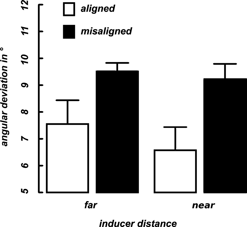
Figure 3. Mean thresholds. Shown are 75% performance thresholds in units of angular deviation from 90° averaged across nine participants as a function of inducer distance (x-axis) and alignment (differently colored bars). Error bars indicate the standard error of the mean for each condition.
Functional Imaging: IC-Related BOLD Signals in the Primary Visual Cortex
We localized our regions of interest in each individual subject (see Materials and methods section). The mean contour and inducer ROIs averaged across the remaining nine participants are depicted in the upper row diagrams of Figures 4 and 5
. We then extracted the spatially and temporally smoothed peristimulus fMRI response evoked by near and far aligned and misaligned stimuli from the voxels of interest using PyNIfTi (http://niftilib.sourceforge.net). Event-related signals spanning a time window of 12 seconds were averaged time-locked to stimulus onset. We included correct and incorrect trials alike. A percent signal change measure was calculated using the following formula: psc = [S(i) – S(1)] × 100/S(1) with S(i) referring to the BOLD signal intensity at time step i after stimulus onset and S(1) referring to the BOLD signal intensity at the first time step. Means and standard errors of the mean were calculated across nine participants at the inducer and contour ROIs in each hemisphere.
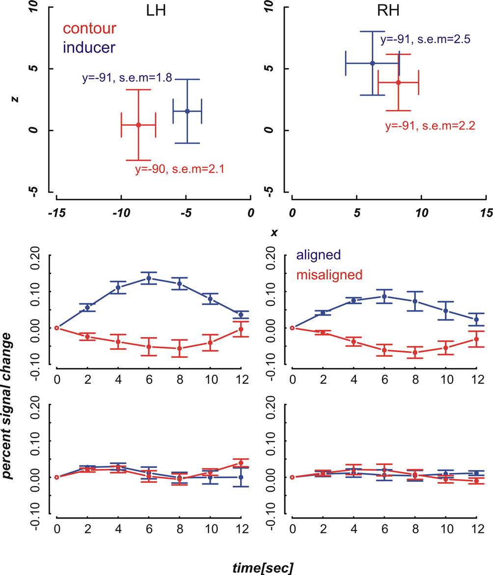
Figure 4. Mean ROI locations and peristimulus plots at ROIs in the far condition. Upper part: Shown are ROI locations of inducers (blue) and contours (red) in the left (LH) and right hemisphere (RH) averaged across nine participants. The plots are analogous to a coronal view with the x-axis representing the left-right and the y-axis representing the ventral-dorsal axis. Error bars show the standard error of the mean, the corresponding MNI coordinates in y-direction are written down close to the data points. Lower part: Plots depict the evoked BOLD changes locked to stimulus onset and spanning a time window of 12 seconds. The upper two graphs show the peristimulus plots at the contour ROIs and the lower two graphs those at the inducer ROIs. Left and right columns show the peristimulus plots in the left and right hemisphere. Error bars represent the standard error of the mean.
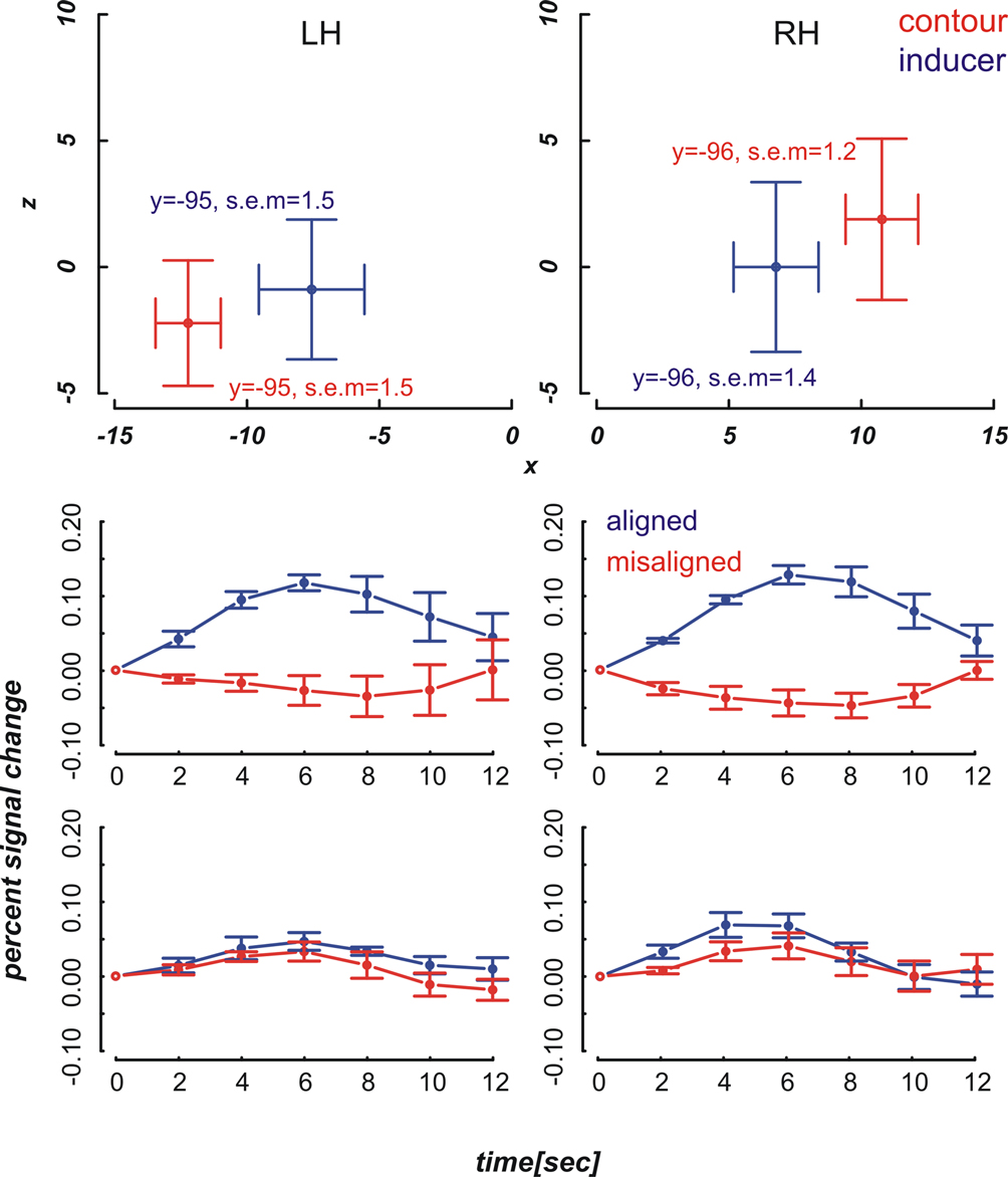
Figure 5. Mean ROI locations and peristimulus plots at ROIs in the near condition. The design of the figures is analogous to that of Figure 4
.
The diagrams in Figures 4 and 5
reveal that the averaged BOLD responses follow the predicted interaction pattern between the stimulus condition and the cortical region of interest: Aligned stimuli evoked stronger BOLD responses than misaligned stimuli at the cortical IC representation, i.e., in striate cortex near the fundus of the calcarine sulcus. In contrast, BOLD activation changes evoked by aligned and misaligned inducers did not markedly differ at the striate locations responsive to inducers. These observations were confirmed by 2 × 2 × 3 repeated measures ANOVAs with the factors ROI (contour vs. inducer) inducer orientation (aligned vs. misaligned) and time step (3, 4, 5) that were performed separately for the near and far condition. Both ANOVAs revealed a main effect for inducer alignment [F(1,8) = 16.46, p = 0.004 and F(1,8) = 24.71, p = 0.001 in the near and far conditions, respectively] indicating that aligned stimuli elicited stronger BOLD changes than misaligned stimuli, and a significant interaction between ROI location and inducer alignment [F(1,8) = 22.28, p = 0.002 and F(1,8) = 27.23, p = 0.001 in the near and far conditions, respectively]. This interaction reflected that BOLD responses to aligned and misaligned stimuli were significantly different from each other at the contour ROI [t_near(8) = 5.10, p < .001, t_far(8) = 5.17, p < .001], but not the inducer ROI.
We compared fMRI BOLD responses in primary visual cortex to subjective contours and control stimuli in areas defined by their responsiveness to physically defined contours and inducers. We had previously shown that retinotopic regions in V1 that respond to real contours are also activated in response to subjective contours after some amount of training (Maertens and Pollmann, 2005
). Here, we observed an increased BOLD response to subjective contour but not to control stimuli (Figures 4 and 5
) in primary visual cortex at locations that were defined by their response to analogous real contours. Primary visual cortex was functionally defined as the area along the calcarine sulcus that extended to the first dorsal and ventral vertical meridian representations (Figure 2
). Activation changes were individually checked to originate from striate cortex by comparing the stimulus ROIs with the meridian mappings. In contrast to the activation pattern at the contour ROI, activation changes evoked by aligned and misaligned inducers did not elicit differential responses at the striate locations responding maximally to the inducers.
The response amplitude in the current study as measured by the percent signal change may appear comparably small, e.g., the maximum response to aligned stimuli at the inducer location does not exceed 14%, whereas in our earlier experiment the maximum response change was about 20%. This may be due to the known reduced functional sensitivity of SE compared with GR-EPI. However, in the absence of large amplitude changes we still obtained a sufficiently high signal to noise ratio to yield significant results. Somewhat unexpectedly, the BOLD signal change in response to the inducers was comparatively small. We suspect that this was due to a temporal overlap between BOLD responses in subsequent trials, which resulted from a larger than expected spatial overlap between inducers in the near and far condition. Even though the activation peaks were separable (Figures 4 and 5
) there was a considerable overlap between responses to near and far inducers. It should be noted that this overlap only affected the inducers, which were present in every trial, but not the activation changes in response to subjective contours, i.e., the comparison between trials with inward- and outward-bound inducers.
There were also no performance differences between the near and far conditions. Even though it has been reported that the perceived strength of subjective contours depends on the support ratio (Kellman and Shipley, 1992
; Ringach and Shapley, 1996
), we did not find any difference between illusory figures with support ratios of .32 and .21 with the parameters used here. Since we did not observe an effect of the support ratio on the behavioral level, there was also no point in checking for differences in BOLD responses to high and low support ratio conditions. Thus, it remains an issue of further study to determine whether there is a quantitative relationship between subjective contour clarity and BOLD responses in V1 or higher visual areas.
Our findings are in apparent contradiction to some of the previous human imaging studies (Hirsch et al., 1995
; Mendola et al., 1999
;Murray et al., 2002
, 2004
; Ritzl et al., 2003
; Stanley and Rubin, 2003
) that did not find indications for subjective contour processing in V1. However, in these studies participants were required to either passively view the stimulus display (Hirsch et al., 1995
; Mendola et al., 1999
; Stanley and Rubin, 2003
) or to detect the presence or absence of a global stimulus shape (Murray et al., 2002
, 2004
; Ritzl et al., 2003
). Our task required participants to specifically focus on the subjective contour compared to the entire subjective figure. It has been shown that the neural processes underlying subjective contour- and figure perception are dissociable (Stanley and Rubin, 2003
) and might involve different neural populations. Whereas neurons at higher levels in the processing hierarchy might respond more to the figural aspects of the Kanizsa stimulus, neurons in early visual cortex provide the higher spatial precision that may be required to resolve differences in the exact path of the subjective boundary. So, paradigms that focus on different aspects of the stimulus are likely to yield different results regarding the underlying neural mechanisms. In addition, it has been suggested that in the process of scene segmentation surfaces or ‘salient regions’ are identified before their exact boundaries (Stanley and Rubin, 2003
). In other words the default mode of processing is crude and limited to figural information (Hochstein and Ahissar, 2002
). Hence, without the particular requirement to discriminate fine spatial differences, subjective contours were unlikely to evoke sufficiently strong activity in V1 to be detected with fMRI. With more sensitive measures it might be possible to observe these responses even in the absence of a particular task (Murray et al., 2006
).
It is unlikely that our results are attributable to differential effects of attentional allocation (e.g., Noesselt et al., 2002
). Since Kanizsa and control stimuli were randomly interleaved, subjects could not know in advance whether attention should be directed to the subjective contour or to the inducers. Now if, regardless of the actual condition, participants were attending toward the subjective contour we should have seen the effect of attention in the subjective contour and in the control condition. However, we found stronger responses only in the subjective contour condition. We can’t of course exclude the possibility that subjective contours are drawing attention, however then attention would only be the consequence of a subjective contour percept and might act to amplify an already evoked subjective contour response.
It remains to be explained how – in the absence of a physical stimulus to the retina and the lateral geniculate nucleus – the subjective contour responses in V1 have been generated. We suggest, as others have done before (Maertens and Pollmann, 2005
; Murray et al., 2004
; Lee and Nguyen, 2001
), that the responses to subjective contours in V1 result from two sources: On the one hand, there are probably lateral interactions between V1 neurons that were excited by the inducers. The known range of lateral connections within V1 is however considerably smaller than the range across which subjective contours have been interpolated in the current experiment (e.g., Angelucci and Bullier, 2003
). Therefore, it is plausible to assume that feedback from extrastriate neurons, which pool information across larger regions of space, also plays an important role in the process of boundary interpolation (Lee and Nguyen, 2001
; Maertens and Pollmann, 2005
; Murray et al., 2004
; Stanley and Rubin, 2003
). In several studies BOLD responses to subjective figure stimuli were observed in regions in the lateral occipital cortex (Hirsch et al., 1995
; Mendola et al., 1999
; Murray et al., 2002
; Ritzl et al., 2003
; Stanley and Rubin, 2003
), which are known to preferentially respond to object-like stimuli (e.g., Malach et al., 1995
). However, activity in these extrastriate regions alone would not be sufficient in itself, because as stated in detail above, it is the functional properties of V1 neurons that enable a crisp subjective contour percept. Hence one could think about a scenario in which neurons in higher visual areas, which respond to the subjective figure, send feedback to retinotopically specific lower visual areas, in which contour responses are being fine-tuned by lateral interactions.
The authors declare that the research was conducted in the absence of any commercial or financial relationships that could be construed as a potential conflict of interest.
The work was supported by a Gertrud Reemtsma fellowship to Marianne Maertens.