1
Rotman Research Institute, Baycrest Centre, Toronto, Canada
2
Department of Psychology, University of Toronto, Canada
Sensitivity to variations in luminance (contrast) is fundamental to perception because contrasts define the edges and textures of visual objects. Recent research has shown that contrast sensitivity, in addition to being controlled by purely stimulus-driven mechanisms, is also affected by expectations and prior knowledge about the contrast of upcoming stimuli. The ability to adjust contrast sensitivity based on expectations and prior knowledge could help to maximize the information extracted when scanning familiar visual scenes. In the present study we used the event-related potentials (ERP) technique to resolve the stages that mediate knowledge-driven aspects of contrast gain control. Using groupwise independent components analysis and multivariate partial least squares, we isolated two robust spatiotemporal patterns of electrical brain activity associated with preparation for upcoming targets whose contrast was predicted by a cue. The patterns were sensitive to the informative value of the cue. When the cues were informative, these patterns were also able to differentiate among cues that predicted low-contrast targets and cues that predicted high-contrast targets. Both patterns were localized to parts of occipitotemporal cortex, and their morphology, latency, and topography resembled P2/N2 and P3 potentials. These two patterns provide electrophysiological markers of knowledge-driven preparation for impending changes in contrast and shed new light on the manner in which top-down factors modulate sensory processing.
A prominent notion in cognitive neuroscience holds that top-down factors such attention, knowledge and expectations can influence how incoming stimuli are processed by sensory systems. Attention-directing cues in visual spatial attention tasks can help the visual system to prepare to process task-relevant information at a particular region of the visual field by biasing cortical excitability (Hillyard and Mangun, 1987
; Hillyard et al., 1998
). The context in which visual input occurs can also influence the subsequent bottom-up analysis via long-range feedback connections (Bullier, 2001
; Bar et al., 2006
; Kveraga et al., 2007a
,b
). In addition, sensory processing may also depend on working memory capacity (Agam and Sekuler, 2007
). In that sense, any prior knowledge or cue that could potentially narrow down stimulus expectations could be beneficial to perception.
Top-down control may be particularly important in the visual system, which must remain sensitive to local variations in luminance (contrast) across the retina. Contrast-sensitive neurons do not respond to stimulation in their receptive field until some threshold contrast level is reached. As stimulus intensity increases above threshold so does the neuron’s rate of firing until it saturates. This dynamic range of contrasts in which the neuron is most sensitive to incremental changes is considerably narrower than the range of contrasts likely to be encountered in typical natural scenes (Albrecht and Hamilton, 1982
; Frazor and Geisler, 2006
). Therefore, contrast-sensitive cells must continually modulate their gain in order to adequately represent local contrast.
Optimal contrast sensitivity is paramount to successful object perception because edges and textures are defined by contrast. This is reflected by the fact that a large portion of neurons in the visual system are sensitive to ambient contrast level, including areas V1, V2, V3a, V4 and MT (Tootell et al., 1995
, 1997
; Boynton et al., 1999
; Avidan et al., 2002
; Gardner et al., 2005
). However, there is a gradual trend towards increasing contrast invariance as one ascends the ventral visual stream, culminating in almost totally contrast-independent responses in higher level object-sensitive areas of the occipitotemporal cortex, such as primate pSTS (Rolls and Baylis, 1986
), lateral occipital complex (LOC) and posterior fusiform gyrus (Avidan et al., 2002
). This trend is likely one facet of object constancy in visual perception (Sary et al., 1993
; Ito et al., 1995
; Grill-Spector et al., 1999
); namely, an increasing capacity to respond to invariant and intrinsic properties of objects, such as their semantic category. Conversely, object-evoked responses in the higher ventral stream areas are less sensitive to transient object properties that depend on viewing conditions, such as luminance contrast across retinal receptive fields, retinal image size and position, etc.
There is much evidence to suggest that contrast sensitivity can be controlled in stimulus-driven fashion (Albrecht and Hamilton, 1982
; Ohzawa et al., 1982
; Ross and Speed, 1991
; Foley, 1994
; Boynton et al., 1999
; Gardner et al., 2005
). For example, if the local ambient contrast at a cell’s receptive field is decreased, contrast gain of that cell tends to be amplified. However, selective attention has also been shown to modulate physiological responses of contrast-sensitive cells as well as the subsequent perceptual experience (apparent contrast). Studies using single-cell recordings have demonstrated that contrast-dependent neuronal responses can also be enhanced by attention (Reynolds et al., 2000
; Martinez-Trujillo and Treue, 2002
). In psychophysical studies, covert shifts of attention – be they transient or sustained – tend to decrease the smallest contrast increment that can be reliably detected (Carrasco et al., 2004
; Huang and Dobkins, 2005
; Ling and Carrasco, 2006
).
Moreover, a recent study behaviourally demonstrated that contrast sensitivity could also be modulated by knowledge and/or expectations about the contrast of an upcoming target (de la Rosa et al., 2009
). Participants identified a series of cued gratings by their contrast. Four gratings in the stimulus set were of low contrast and were difficult to identify, while a fifth grating had extremely high contrast and was easy to identify. In the Baseline condition only the four low-contrast gratings were presented. In another condition (Uninformative cue) the high-contrast grating was also presented, but was unpredictable. In the third condition (Informative cue) the high-contrast grating was predicted by a cue. The identity of the specific low-contrast grating was unpredictable in all conditions. Participants’ contrast sensitivity (indexed by their ability to correctly identify low-contrast gratings) was assessed while systematically manipulating the predictability of a high-contrast grating. The addition of an occasional unpredictable high-contrast grating to the stimulus set adversely affected identification accuracy for low contrast gratings relative to the condition in which only the low-contrast gratings are presented. However, when the high-contrast grating was made predictable by the cue, there was no such accuracy cost. This suggested that knowledge conferred by the cue was used to tune contrast sensitivity on each trial. This mechanism could potentially serve to maximize discriminability when an observer is scanning a familiar visual scene by using prior knowledge to match contrast sensitivity to impending changes in contrast.
In the present investigation we used the event-related potentials (ERP) technique in conjunction with the cued absolute identification paradigm described by de la Rosa et al. (2009)
to resolve stages of information processing in the brain that facilitate such knowledge-driven sensory gain control. Namely, we sought to isolate spatiotemporal patterns of brain activity related to cue-driven preparation rather than the evoked responses to the targets themselves.
First, we hypothesized that any such activity should differentiate conditions according to the informative value of the cue rather than the ability of the participants to identify gratings. In other words, cue-locked activity should differ between the Informative condition on one hand and the Baseline/Uninformative conditions on the other, despite the fact that the Baseline and Informative conditions cannot be distinguished in terms of accuracy. This task contrast, if it exists, would reflect the difference between using the cue and not using the cue to adjust sensitivity.
Second, if participants utilize the cue in the Informative condition to increase or decrease their sensitivity, then any activity related to top-down preparation should also differentiate trials based on the identity of the cue, but only when the cue is informative. In other words, we should be able to isolate differences between cues that signal low contrasts versus cues that signal high contrasts, but only in the Informative condition. This contrast would reflect the difference between using the cue to shift sensitivity towards lower versus higher contrasts. Note that these hypothesized task differences reflect overlapping stages of processing. If both could be isolated, then owing to their functional similarities it is likely that they would overlap spatially and temporally. Given that the meaning of the cue must be processed for it to confer any predictive advantage, we expected the task-relevant potentials to comprise mostly late endogenous responses (>200 ms following cue onset).
One purpose of a top-down control system for contrast gain may be to allow representations of objects in higher areas to remain invariant across different viewing conditions, including varying levels of illumination. Therefore, areas most involved in knowledge-driven gain adjustments may be those whose responses typically do not depend as much on ambient contrast, such as LOC or posterior fusiform gyrus (Avidan et al., 2002
).
Our experimental question was framed in terms of concrete task differences, but the absolute latency or spatial distribution of those differences was difficult to predict because we used a novel paradigm that had not been previously studied using neuroimaging techniques. Rather than confine our analysis to a few select peaks and electrodes and potentially miss interesting task effects, we chose a multivariate analytic approach (spatiotemporal partial least squares; ST-PLS) (McIntosh et al., 1996
; McIntosh and Lobaugh, 2004
) that allowed us to detect patterns of task-modulated activity simultaneously across both the spatial and temporal domains and to restrict those patterns by hypothesized task effects. Moreover, we sought to resolve these patterns into component processes. To this end, prior to statistical analysis data were subjected to groupwise independent component analysis (ICA) (Kovacevic and McIntosh, 2007
). This served to create an alternate spatial representation of the EEG signal in which task effects could be assessed across components with maximally temporally independent time courses. Since independence is maximized in a temporal sense, this technique was ideally suited to studying how experimental effects are expressed across distinct stages of information processing. Data compression by ICA has been shown to yield more robust statistical effects in subsequent statistical analyses and the combined groupwise ICA/ST-PLS approach has recently proven fruitful in studying cue-driven processes in both auditory and visual modalities (Kovacevic and McIntosh, 2007
; Diaconescu et al., 2008
). We used standardized low resolution electromagnetic tomography (sLORETA) (Pascual-Marqui, 2002
) for cortical source localization of task-relevant components.
In this paper we also consider an alternative hypothesis for the effect reported by de la Rosa et al. (2009)
, which posits that participants do not use the informative cue to modulate contrast gain, but rather to avoid the occurrence of the high-contrast grating, perhaps by blinking, by moving their eyes or by “defocusing” attention. In this view, gain is at a constant level in all conditions but sensitivity is adversely affected by an unpredictable high-contrast grating which saturates neuronal responses. Therefore, high-contrast stimuli impair accuracy for all stimuli in the Uninformative condition but they have no effect in the Informative condition because they can be avoided. The control experiment was designed to behaviourally test this hypothesis by forcing participants to make a perceptual judgment about high- and low-contrast stimuli.
Participants
Fifteen naïve, healthy young adults (eight female, 19–29 years old, mean = 23.6, standard deviation = 2.92 years) participated in the ERP experiment. Five participants took part in the behavioural control experiment (two female, 18–27 years old, mean = 23.0, standard deviation = 3.61 years). Participants were recruited from the volunteer pool of the Rotman Research Institute at Baycrest Centre. All participants were right-handed and reported normal or corrected-to-normal vision. Experiments were performed with the informed consent of each individual in accordance with the joint Baycrest Centre-University of Toronto Research Ethics Committee.
Stimuli and Task
The target stimuli were a set of three vertical sinusoidal gratings generated in MATLAB (Mathworks, Inc.), using the Psychophysics Toolbox extension (Brainard, 1997
). The gratings were identical in all physical characteristics (5 × 5° visual angle, spatial frequency 4 cpd and phase equal to zero) save for contrast, such that two gratings had relatively low contrast (19% and 26%) while the third had high contrast (100%). Contrast was measured using the Michelson formula (Michelson, 1927
):

This manipulation served not only to create a high-low separation within the set, but also to increase the difficulty of correctly identifying low-contrast gratings, because they were more similar to each other than to the high-contrast grating.
Participants were comfortably seated in a dimly-lit and double-walled sound-attenuated chamber (IAC model 1204A) in the Rotman Research Institute at Baycrest Centre, at a viewing distance of 60 cm from a Sony Trinitron GDM-F520 computer screen while stimuli were presented centrally over a uniform grey background (luminance: 55.16 cd/m2). In each trial a symbolic cue was presented first for 550 ms (Figure 1
). The cue could be either a cross (“+”) or a letter “H”. Following an inter-stimulus interval (ISI) equal to 500 ms, a target sinusoidal grating was presented for 500 ms. The task was to correctly identify the grating by the relative magnitude of its contrast, using a number key on a keyboard. The 19%-, 26%- and 100%-contrast gratings corresponded to keys numbered 1, 2 and 3, respectively. The response period was limited to 2 s following the onset of the target grating. Participants were instructed to respond as accurately as possible. At the end of the response period participants were shown the correct number of the grating (1, 2 or 3, presented for 500 ms), regardless of whether their response on that trial was correct or incorrect. To reduce expectancy effects, the trials were jittered such that the inter-trial interval between the offset of the feedback stimulus at the end of one trial and the onset of the cue at the start of the next trial was varied randomly and with equal probability between 800 and 1200 ms.
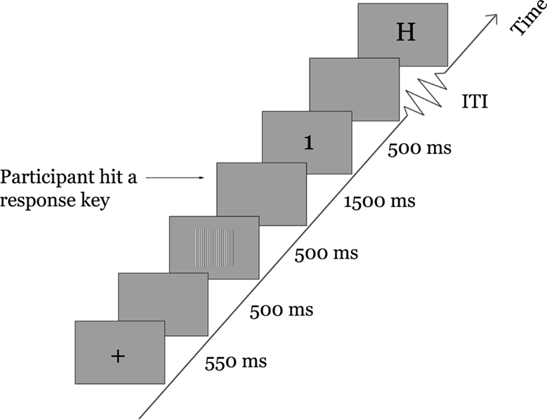
Figure 1. Task schematic.
Trials were organized into condition-specific runs that differed in terms of target sets and the informative value of the cues. In the Baseline (B) condition, only the two low-contrast gratings (19% and 26%) could appear on any given trial (Figure 2
). In the Informative-Cue (IC) and Uninformative-Cue (UC) conditions all three gratings (19%, 26% and 100%) could appear. Each grating was presented 66 times in each condition, across two runs. Thus, Baseline consisted of 132 trials, while the Informative- and Uninformative-Cue conditions consisted of 198 trials each.
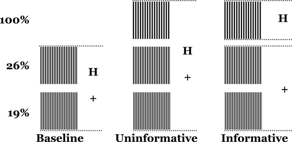
Figure 2. Experimental conditions. Baseline: only the two low-contrast gratings appear and the cues are unpredictive. Uninformative: all three gratings appear and the cues are unpredictive. Informative: all three gratings appear, “+” predicts low-contrast gratings, “H” predicts the high-contrast grating.
In both the Baseline and Uninformative-Cue conditions, the “H” cue was randomly assigned to precede 16 of the 66 presentations of each grating, while the “+” cue was assigned to precede the other 50 presentations. In other words, the “H” cue appeared on 25% of the trials and the “+” cue appeared on 75% of the trials. This random and equiprobable assignment ensured that the cues were uninformative and could not be used to predict the stimulus contrast. In the Informative-Cue condition the “H” cue was always assigned to trials in which the high-contrast grating would be presented and the “+” cue was always assigned to trials in which the low-contrast gratings would be presented. Therefore, the cues were informative in each trial because they could be used to predict whether the contrast of the ensuing stimulus would be high or low.
Participants were verbally advised about cue validity prior to each run. Each participant completed 66 Baseline trials as a practice block (discarded from the analysis) as well as two consecutive runs of each condition. All participants initially completed two Baseline runs, while the order of the subsequent condition-specific pairs of runs was counterbalanced across participants. Thus, each participant completed a total of 66 practice trials and 528 experimental trials.
Electrophysiological Signal Acquisition and Processing
The electroencephalogram (EEG) was continuously recorded from 76 scalp locations using Ag/Ag-Cl-tipped electrodes attached to a custom cap according to the international 10/20 system and digitized at a rate of 512 Hz. Recordings were made using the Active-Two system (BioSemi, Amsterdam, The Netherlands) which does not require impedance measurements or an online reference. Offsets from the common mode were no greater than 25 mV across all electrodes. All offline signal processing and artifact correction was performed using EEGLAB software (Delorme and Makeig, 2004
). Continuous recordings were downsampled to 256 Hz, average-referenced and digitally filtered [band-pass: 0.1–100 Hz; notch: 60 Hz]. Data were then epoched and baselined into [−200 1950] ms segments with a [−200 0] ms pre-cue baseline. Trials with excessive signal amplitude were rejected first, leaving between 469 and 518 trials and an average of 493 trials per subject. Ocular and muscle artifacts were identified and subtracted from the remaining trials on a subject-by-subject basis using ICA (Delorme and Makeig, 2004
). Both correct- and incorrect-response trials were analyzed.
Groupwise Independent Component Analysis
The term “groupwise” refers to the fact that the ICA decomposition was performed simultaneously across all subjects and all conditions (Kovacevic and McIntosh, 2007
). Data from all participants were concatenated and the optimal number of underlying dimensions for the whole dataset was determined using the Bayesian Information Criterion (BIC) (Hansen and Yu, 2001
). A model with nine dimensions yielded the maximum BIC probability. Concatenated data were first subjected to principal components analysis (PCA) for spatial dimensionality reduction and then decomposed using the Infomax ICA algorithm, as implemented in EEGLAB (Delorme and Makeig, 2004
). Thus, single-trial data from a space of 76 electrodes were re-expressed in the space spanned by the independent components. Subject- and condition-specific single-trial time series were calculated for each component by multiplying the corresponding time series in electrode space by the ICA mixing matrix. The resulting single-trial component activations were averaged across trials to yield condition-specific independent component waveforms for each participant.
Spatiotemporal Partial Least Squares
Task ST-PLS
Spatiotemporal partial least squares (ST-PLS) analysis is a multivariate statistical technique that can be used in the context of neuroimaging to relate a set of design variables (e.g. conditions) to a set of brain activity measures (e.g. scalp potentials) (McIntosh et al., 1996
). As such, ST-PLS represents a useful method of extracting distributed activity patterns that vary linearly across time in a task-dependent manner. In multivariate terminology these relationships are referred to as latent variables (LVs). When applied to ERPs, each LV derived from the analysis represents one contrast between experimental conditions (design saliences) in relation to a particular pattern of electrodes and latencies that optimally expresses that contrast (electrode saliences) (Lobaugh et al., 2001
). In the present analysis, independent components were used as an alternative spatial representation of the ERP data, so ST-PLS was used to identify task-dependent spatial patterns in terms of electrodes in one analysis and in terms of independent components in another (Kovacevic and McIntosh, 2007
).
Experimental effects captured by each LV were statistically assessed using resampling procedures. First, the significance of each task effect was determined using permutation tests (Edgington, 1995
). Each permuted sample was obtained by random sampling without replacement to reassign the order of conditions within participants (500 replications). Second, the stability of each task effect was indexed at all data points across participants using bootstrap resampling to estimate standard errors of the corresponding electrode saliences (Efron and Tibshirani, 1986
). Bootstrap samples were generated by random sampling with replacement of participants within conditions (500 replications). Assuming a Gaussian bootstrap distribution, the ratio of an electrode salience to its standard error is approximately equivalent to a z score. Bootstrap ratios were thresholded across all data points to allow parsimonious identification of spatiotemporal patterns that reliably expressed each task effect. Ratios greater than 3.0 (roughly equivalent to a 99% confidence interval) were taken to indicate stable saliences, i.e. time points at which the task effect was reliable.
ST-PLS is typically applied in data-driven fashion such that task effects are partially determined by the most robust spatiotemporal patterns in the data. However, there is a variant that allows spatiotemporal patterns to be mapped directly to a set of a priori contrasts, termed “non-rotated” ST-PLS (McIntosh and Lobaugh, 2004
). In this version of ST-PLS the contrasts served to restrict the time-varying patterns of activity derived from the analysis. Each contrast represented a particular differentiation of component signal amplitude across conditions.
In order to explore cue-driven brain activity independently of the subsequent target stimulus, all analyses were limited to [−200 1050] ms epochs ranging from cue onset to grating onset, with a −200-ms pre-cue baseline. In the first analysis we examined which aspects of brain activity were sensitive to the informative value of the cue. Component activations in the IC condition were contrasted with those in the UC/B conditions, coded as [1 −1 −1]. This analysis was limited to “+” cue trial types because they were more numerous and to ensure that the epochs to be compared were time-locked to stimuli with identical physical characteristics. In the second analysis we attempted to isolate those features of the EEG signal that were sensitive to cue identity and unique to the IC condition. We contrasted “+” versus “H” cue trials and ran ST-PLS separately for the IC condition (coded [1 −1]) and for the the UC/B conditions (coded [1 −1 1 −1]).
Behaviourally, participants showed evidence of preparation only in the IC condition. The nature of this preparation (increased or decreased contrast sensitivity) must depend on the identity of the cue. Therefore, spatiotemporal patterns of brain activity related to cue-driven preparation should (a) be sensitive to the difference between cues with different identities and (b) only materialize when those cues are informative. In other words, any spatiotemporal patterns that differentiate trial types only in the IC condition must serve some gain adjustment function.
Behaviour ST-PLS
Task ST-PLS analysis allowed us to examine how ERP amplitude was affected by the informative value of the cue. As a final step, we sought to determine whether task-dependent changes in the spatiotemporal pattern of electrical activity following the cue presentation could predict subsequent identification accuracy. Behaviour ST-PLS (McIntosh and Lobaugh, 2004
) was used to identify task-dependent changes in brain-behaviour correlations. Identification accuracies were expressed as z-scores using subject-specific mean and standard deviation and correlated with independent component amplitude across participants within task. The resulting correlation matrix was subjected to SVD as described above. Significance and stability of statistical effects were estimated using the same permutation test and bootstrapping procedure.
Standardized Low Resolution Electromagnetic Tomography
We used standardized low resolution electromagnetic tomography (sLORETA) (Fuchs et al., 2002
; Pascual-Marqui, 2002
; Jurcak et al., 2007
) to estimate source activity for task-relevant components based on their scalp maps. The sLORETA algorithm is a modified weighted minimum norm approach to the inverse problem. To produce a single discrete linear solution, the algorithm works under the constraint that source activity be as smoothly distributed as possible. It has been shown to localize point sources with zero error under ideal conditions (Sekihara et al., 2005
). We chose to localize independent components instead of ERP peaks because tomographic solutions based on factor scores tend to be less noisy than those based on mean or peak voltage (Carretié et al., 2004
). Solutions were expressed in the MNI152 human brain volume with 6239 cortical grey matter voxels at 5 mm resolution.
Control Experiment
This behavioral control experiment was similar to the procedure described above with one important change. A second high-contrast (79%) grating was added to the stimulus sets in the Uninformative- and Informative-Cue conditions, such that there were two equiprobable high-contrast gratings (79% and 100%; stimuli 3 and 4, respectively). The task was identical to Experiment I in all other aspects. In other words, in the Informative-Cue condition the “H” cue still accurately predicted the onset of a high-contrast stimulus. However, the cue could not be solely used to identify the grating. Participants had to attend to a grating in order to judge its contrast.
Behaviour
In the main ERP experiment, identification accuracy for the high-contrast stimulus was extremely high in both IC and UC conditions (>99%) and participants reported no difficulty in identifying it. Identification accuracy for the low-contrast gratings was subjected to a series of paired t-tests which revealed no significant difference between the B and IC conditions [t(14) = 0.66, p = 0.52]. However, there were significant differences between the B and UC conditions [t(14) = 3.40, p = 0.004], as well as between the IC and UC conditions [t(14) = 3.58, p = 0.003]. These data are displayed in Figure 3
.
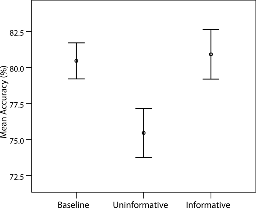
Figure 3. Mean identification accuracy for low-contrast gratings. Bars indicate standard errors of the mean.
In the control experiment, identification accuracy for high-contrast gratings was above-chance in both UC (67.4%) and IC (72.5%) conditions. Importantly, the main behavioral effect for low-contrast gratings was still present. No significant differences were detected between the B and IC conditions [t(4) = 1.01, p = 0.37]. There were significant differences between the B and UC conditions [t(4) = 3.98, p = 0.016], as well as between the IC and UC conditions [t(4) = 3.37, p = 0.028].
ST-PLS Analysis in Electrode Space
Informative versus uninformative/baseline contrast
The contrast between IC and UC/B conditions was statistically significant by permutation test (p = 0.03). This task effect indicated the presence of scalp potentials that differentiated the IC condition from UC/B. Figure 4
shows that the contrast was expressed at two distinct topographic regions. The first was over bilateral parietal-occipital channels, where differences materialized 190 ms following cue onset and remained stable until approximately 600 ms. This effect appears to map onto amplitude differences across the P2-N2-P3 components. Specifically, amplitude in the IC condition was attenuated relative to UC/B. A complementary expression of the effect was also observed at the vertex, emerging 210–600 ms following cue onset. Here, the effect was polarity-reversed relative to the parietal-occipital channels, such that task differences mapped onto weaker negative potentials in the IC condition compared with the UC/B conditions. The average waveforms during this period comprised an initial negative peak at 250 ms and a positive peak at 300 ms, followed by a negative slow wave. Note that these statistical contrasts were assessed by permuting squared singular values, so the tests were effectively two-tailed. For this reason, the sign of the statistical contrast is not important: an effect would be significant whether the IC condition had greater or smaller amplitude than the UC/B conditions.
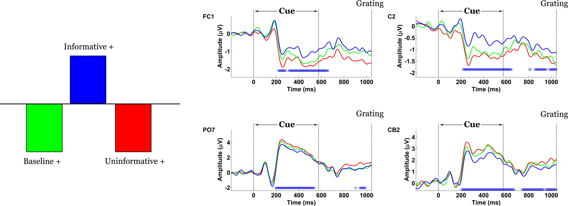
Figure 4. Spatiotemporal patterns of scalp activity that differentiate Informative and Uninformative/Baseline conditions. Left: schematic indicates how the statistical contrast was coded. Right: condition-specific ERPs time-locked to cue onset and averaged across “+” cue trials, shown separately for four representative electrodes. Blue dots above the abscissa indicate time points at which the statistical contrast is reliable by bootstrap test.
The inclusion of several distinct deflections in this experimental effect suggested that the statistical contrast captured by the LV may be a consequence of task differences across more than one underlying electrogenic process. Indeed, the amplitude distribution of difference waves computed from the B and IC conditions was time-dependent, with a posterior-going shift from 250 to 330 ms.
“+” versus “H” contrast
In order to test whether the cue elicited any preparatory activity unique to the IC condition, data time-locked to the cue were organized into condition- and cue-specific blocks (across high- and low-contrast trials). Non-rotated ST-PLS analyses were designed to contrast brain responses to the two cues (“+” versus “H”), separately for the B and UC conditions on one hand and for the IC condition on the other. In both instances, task differences were significant by permutation test (p = 0) and most stable over central (Cz/1/2/3/4) and central-parietal channels (CPz/1/2/3/4) (Figure 5
). In all conditions the difference manifested as a higher-amplitude P3-like wave in the “H”-cue trials with peak latency at approximately 500 ms. However, the magnitude of the difference was greater in the Valid-Cue condition.
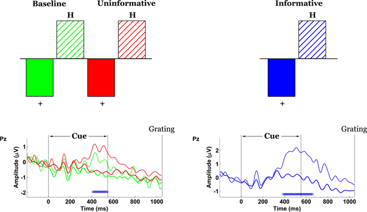
Figure 5. Spatiotemporal patterns of scalp activity that differentiate “+” cue and “H” cue trials, separately for the Uninformative/Baseline conditions and for the Informative condition. Top: schematic indicates how the statistical contrasts were coded. Cue- and condition-specific ERPs time-locked to cue onset, shown for electrode Pz. Blue dots above the abscissa indicate time points at which the statistical contrast is reliable by bootstrap test.
ST-PLS Analysis in Independent Component Space
Electrode-space analyses revealed significant effects of experimental condition, but it was unclear whether those effects could be attributed to a single underlying process or several. Groupwise ICA served to represent the signal from 76 electrodes in a space of nine maximally independent components. Of those components, only four (1, 3, 6 and 9) displayed task-related amplitude differentiation.
Informative versus uninformative/baseline contrast
The contrast between IC and UC/B conditions remained statistically significant by permutation test (p = 0). This task effect indicated the presence of scalp potentials that differentiated the IC condition from the others and was primarily expressed by components 1 and 3 (Figure 6
). Component 1 weighted cerebellar, occipital and parietal electrodes most heavily and more so on the left side than the right. Component 3 was mainly distributed over central-parietal electrodes.
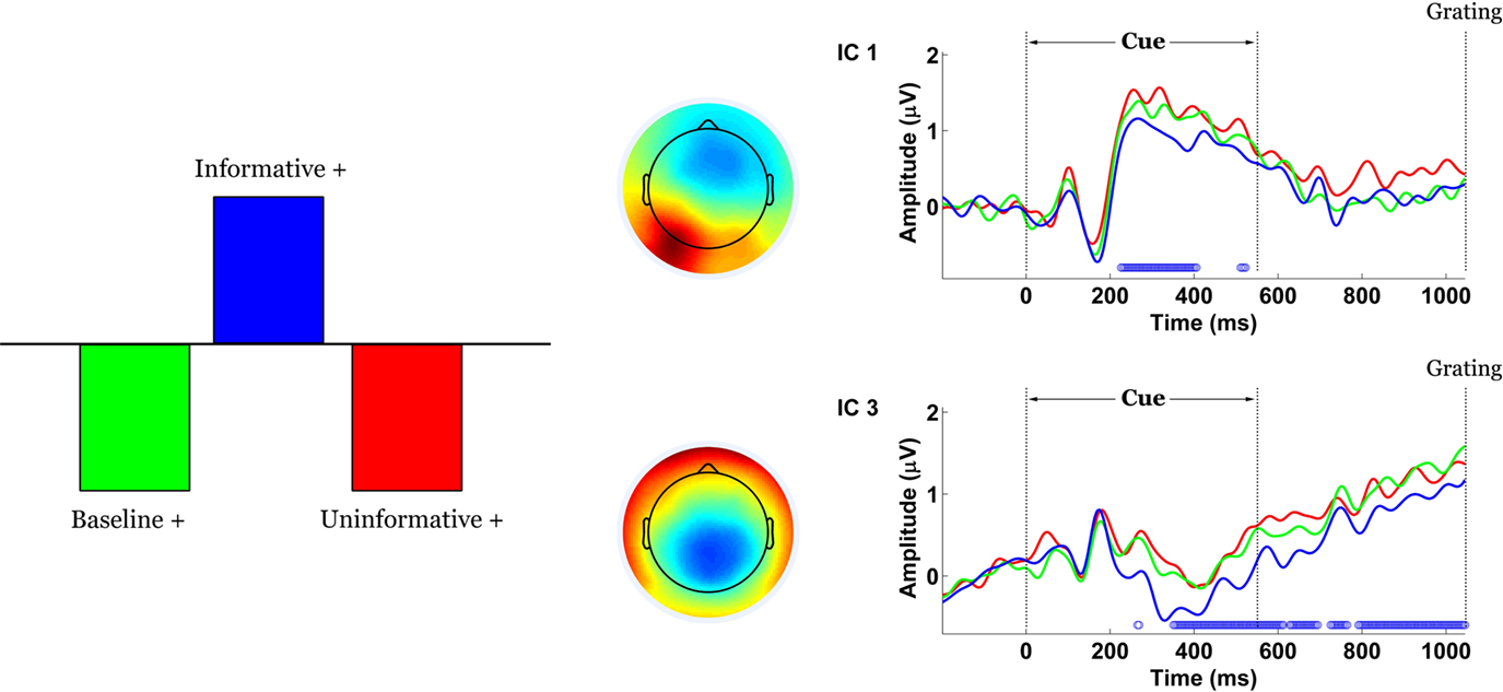
Figure 6. Spatiotemporal patterns of scalp activity that differentiate Informative and Uninformative/Baseline conditions. Left: schematic indicates how the statistical contrast was coded. Middle: colour-coded topomaps indicate the weights in the ICA mixing matrix. Warmer colours represent positive weights. Right: condition-specific ERPs time-locked to cue onset and averaged across “+” cue trials, shown separately for each component. Blue dots above the abscissa indicate time points at which the statistical contrast is reliable by bootstrap test.
Both components displayed stimulus-locked P1-N1 responses that were not task-dependent, as well an offset response roughly 650–750 ms post-cue (150–250 ms following cue offset). Component 1 captured an early and relatively brief expression of the effect, with stable bootstrap ratios ranging from 210 to 400 ms following cue onset. Component 3 captured a sustained later expression of the effect, from 350 ms post-cue until the onset of the grating. Please note the brief temporal overlap between the component-specific effects, from approximately 350 to 400 ms post-cue. For both components, the effect can be attributed mainly to amplitude differences as opposed to latency shifts. Specifically, task-related potentials associated with IC were of smaller absolute magnitude than UC/B in component 1, and of larger magnitude than UC/B in component 3.
The task-related potentials of components 1 and 3 morphologically resemble the visual P2-N2 complex and the P3 evoked potentials commonly observed in the literature. This is consistent with their respective latencies and topography (Simson et al., 1977
). However, we must exercise caution when attempting to describe wave morphology of ICA-decomposed signals in terms of evoked potentials observed in the electrodes. For example, the polarity of component activations is often reversed since the electrodes that contribute to that signal may have been assigned negative weights in the decomposition. This is probably the case for component 3, which is mainly comprised of negatively-weighted electrodes from central-parietal regions. Hence, the negative-going deflection observed at approximately 400 ms post-stimulus most likely corresponds to a positive-going deflection at those electrodes.
“+” versus “H” contrast
Contrasts between the two cues (“+” versus “H”) were assessed separately for the UC/B conditions and for the IC condition. In both cases, the contrasts were significant (p = 0) and were expressed over two common components (components 6 and 9). An additional pair of components (components 1 and 3, Figure 7
) captured the contrast only for IC but not for the UC/B conditions. Note that these were the same components that differentiated the IC condition from the others. In this instance their time courses overlapped considerably, expressing the contrast at 500–850 ms (component 1) and 400–850 ms (component 3).
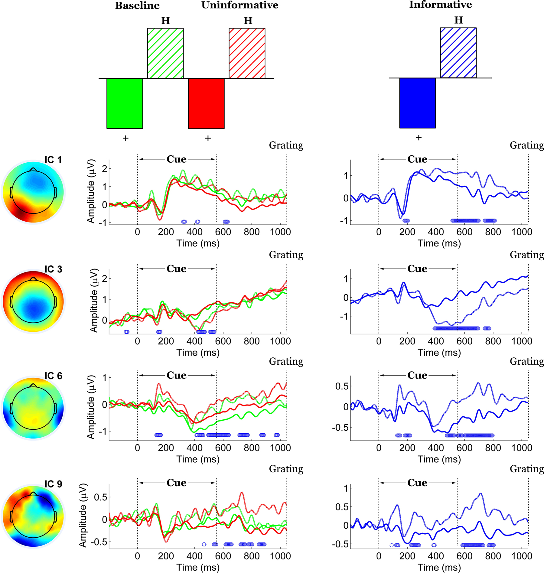
Figure 7. Spatiotemporal patterns of scalp activity that differentiate “+” cue and “H” cue trials, separately for the Uninformative/Baseline conditions and for the Informative condition. Top: schematic indicates how the statistical contrasts were coded. Cue- and condition-specific ERPs time-locked to cue onset, shown separately for each component. Blue dots above the abscissa indicate time points at which the statistical contrast is reliable by bootstrap test.
Of the two components that expressed the contrast across all conditions, component 6 captured a central-parietal expression of the effect together with some contribution from bilateral temporal-occipital sites. The spatial distribution of component 9 was irregular and difficult to interpret, involving contributions from posterior as well as lateral frontal electrodes. As the last component derived from the decomposition it captured the least proportion of total variance. These two components reliably expressed the effect at latencies that were roughly comparable, from 400 to 900 ms following cue onset. In addition, component 6 displayed a brief epoch of stability roughly 100 to 200 ms post-cue.
Behaviour ST-PLS
The cue-locked signal from component 3 was significantly correlated with identification accuracy (p = 0) and was stable at 230–430 ms (Figure 8
, middle). The pattern did not differentiate among conditions and instead displayed a positive association between amplitude and accuracy across all three tasks (B 0.804, UC 0.698, IC 0.575) (Figure 8
, right). Accuracy did not correlate with activity in any other components, including component 1.
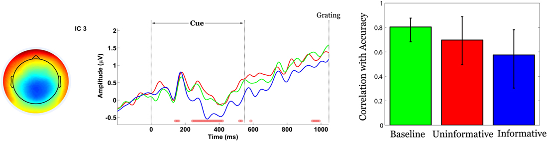
Figure 8. Brain-behaviour relationships (Behaviour ST-PLS). Left: colour-coded topomap of component 3 indicates the weights in the ICA mixing matrix. Warmer colours represent positive weights. Middle: condition-specific component activation time-locked to cue onset. Green, red and blue lines correspond to B, UC and IC conditions, respectively. Red dots above the abscissa indicate time points at which the correlation pattern is reliable by bootstrap test. Right: Correlation between component amplitude and identification accuracy.
Source Analysis
sLORETA solutions were derived for components 1 and 3 and are displayed on an MNI152 T2-weighted template. Broadly speaking, both components were localized to the inferior occipitotemporal cortices, though component 1 was more posterior and left lateralized, while component 3 was anterior and distributed bilaterally. Component 1 was associated with activity mainly in the left fusiform gyrus (BA 37, 19) (X,Y,Z) = (−45,−60,−25) (Figure 9
, top). Component 3 comprised the inferior temporal gyrus (BA 20) (X,Y,Z) = (50,−10,−40), fusiform gyrus (BA 37) (X,Y,Z) = (55,−55,−25) and middle temporal gyrus (BA 21) (X,Y,Z) = (50,5,−40) (Figure 9
, bottom).
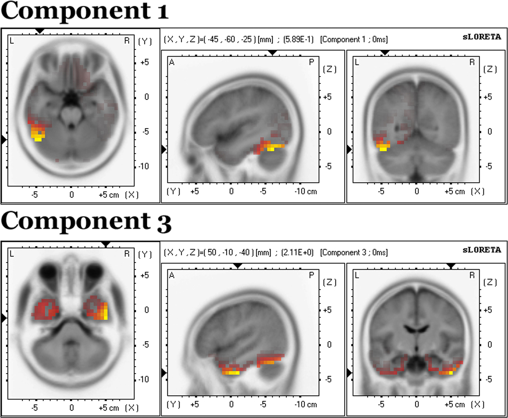
Figure 9. Source localization from sLORETA for components 1 (top) and 3 (bottom). The solution is displayed on an MNI152 T2-weighted template.
The behavioral results confirm that information conferred by the cue mediates sensitivity to the contrast of an upcoming target. The addition of an unpredictable high-contrast grating in the UC condition was associated with decreased identification accuracy for low-contrast gratings relative to Baseline, presumably because of a tonic reduction in sensory gain. When the high-contrast grating was made predictable as in the IC condition, identification accuracy for low-contrast gratings recovered to Baseline levels. The introduction of a fully informative cue for high-contrast gratings allowed flexible tuning of sensory gain on a trial to trial basis such that task performance could be maintained at optimal levels due to enhanced contrast sensitivity on low-contrast trials while sensory overload could be prevented by diminished sensitivity on high-contrast trials (de la Rosa et al., 2009
). The alternative view that the cue was utilized as part of an avoidance strategy was shown to be untenable by the control experiment because the effect persevered even when participants were forced to make a perceptual decision about high-contrast stimuli (which they succeeded in doing at above-chance levels).
The ERP data clearly identify those aspects of brain activity that are sensitive to cues bearing information about the contrast of upcoming targets. Electrode analysis revealed that the P2, N2 and P3 components of the ERP waveform were all modulated by task. However, it was unclear whether these multiple peaks represented a unitary process or several stages of processing. Further, we also predicted that the brain should be sensitive to individual cues only when they are predictive but electrode analysis could not validate this claim, because contrasts between “+” and “H” trials were statistically significant across all three conditions, despite the fact that they were qualitatively different in IC compared to UC/B. Therefore, we used groupwise ICA as a method of parsing the signal into an alternate spatial representation of temporally independent components.
As predicted, analyses in component space revealed two robust spatiotemporal patterns of scalp potentials that differentiated among conditions based on the predictive value of the cue. Furthermore, when the cues were predictive, these patterns were also sensitive to the identity of cues. The fact that the two task contrasts were expressed by common components is consistent with the notion that they capture overlapping aspects of function. The first component displayed a posterior occipital-cerebellar distribution and encompassed a biphasic peak complex roughly 200–300 ms post-stimulus. The second component had a central-parietal distribution and comprised a main broad peak at 400 ms post-stimulus. In terms of their morphology, topography and latency, the two components appear to be similar to the classical visual P2/N2 and P3 peaks (Simson et al., 1977
), though we cannot guarantee that they are homologous. The relatively long-latency P3 is consistent with previous literature (Simson et al., 1977
; Squires et al., 1977
; Perrault and Picton, 1984
). The fact that an N2-like and a P3-like potential were captured by different components is consistent with the long-held view that they are generated by at least two independent sources.
The emergence of endogenous potentials typically signals broad stages of cognitive processing (Hillyard and Picton, 1987
). The N2 is associated with registering the onset of an informative stimulus (Picton and Hillyard, 1974
), as well as with perceptual stimulus evaluation and classification (Ritter et al., 1979
) because it has a modality-dependent topography (Simson et al., 1977
). The P3 represents a set of later, more involved evaluative steps (Picton, 1992
) that are generally thought to index the updating of context (Donchin, 1981
; Donchin and Coles, 1988
).
This work complements a growing literature on top-down factors and the way in which they influence sensory processing. For example, one prominent notion holds that visual spatial selective attention facilitates sensory processing by modulating gain in visual cortex (Hillyard and Mangun, 1987
; Hillyard et al., 1998
). The task-related components observed in this study bear some resemblance to potentials evoked by attention-directing cues (Harter et al., 1989
; Harter and Anllo-Vento, 1991
; Hopf and Mangun, 2000
). The early directing attention negativity (EDAN) is usually observed 200–400 ms following cue onset and is most prominent at occipital-parietal channels on the hemisphere contralateral to the direction indicated by the cue. It has been hypothesized that EDAN reflects the interpretation of the symbolic cue and the orienting of attention. Approximately 500 ms following cue onset, posterior electrodes contralateral to the cued direction also become more positive compared to those on the ipsilateral side. This late directing attention positivity (LDAP) is typically sustained until target onset and is thought to reflect gain control in cortical structures preparing to process relevant visual information.
At first blush, comparisons between these results and our own appear difficult for two reasons. First, in the present study all stimuli were centrally presented and it is unlikely that spatial attention demands differed across conditions (de la Rosa et al., 2009
). This is corroborated by the control study, which demonstrated that attention was deployed in the same manner across all gratings and conditions. Second, EDAN and LDAP are, by definition, lateralized and differ somewhat from components 1 and 3 in terms of topography. However, components 1 and 3 are similar to EDAN and LDAP in the sense that both pairs comprise an early, relatively transient potential in tandem with a long-latency potential that is sustained at least until target onset. Moreover, efforts to determine where sensory gain is modulated by spatial attention have consistently implicated fusiform gyrus and extrastriate regions (Gomez-Gonzales et al., 1994
; Heinze et al., 1994
), in concordance with our source analysis.
These similarities suggest that the functional interpretation of components 1 and 3 may be similar to EDAN and LDAP. Component 1 may reflect an early stage in which the brain registers the onset of an informative event, whereas the late sustained component 3 could reflect the modulation of cortical excitability. Though this explanation must be rigorously tested in future studies, it is at least consistent with our Behaviour ST-PLS analysis which established a linear relationship between brain activity and identification accuracy for component 3 but not component 1. If the activity captured by the first component is associated with registering the onset of the the cue, then it does not necessarily follow that greater or smaller amplitude would be associated with a change in sensitivity. Noting the presence of the cue and interpreting its meaning is trivial (see the following paragraph) so the amplitude of that component may not influence accuracy. On the other hand, if component 3 is associated with changes in gain then its amplitude should directly influence accuracy, consistent with the Behaviour ST-PLS results.
Top-down effects have also been studied from the perspective of stimulus expectation and prediction. Top-down feedback may help to guide and constrain the bottom-up analysis (Bullier, 2001
; Kveraga et al., 2007b
). For example, there is evidence to suggest that the context in which an object is perceived can be utilized to make top-down predictions about the identity of that object and to aid recognition by narrowing down the range of possibilities generated by the bottom-up analysis in the ventral stream (Bar et al., 2006
; Kveraga et al., 2007a
). However, note that the pattern of results that we observed cannot be accounted for in this manner. It is unlikely that the informative cue helped participants to narrow down the range of possibilities because identification accuracy for the high-contrast grating was near-perfect (>99%) in both the informative and uninformative conditions. Likewise, the vast majority (>98%) of errors in the low-contrast trials were due to the low-contrast gratings being mis-identified as each other. This strongly implies that participants were well-capable of categorizing gratings as “low” or “high” contrast, regardless of whether the cue was informative or uninformative. In other words, working memory requirements were comparable in the two tasks. Therefore, task differences probably do not reflect the ability of participants to narrow down stimulus expectations, but rather their sensitivity.
Is the perception of visual contrast a unique instance in which prior knowledge and context modulate sensory processing, or does their influence extend across other sensory modalities? Research in auditory psychophysics has demonstrated similar effects in the perception of loudness (Parker and Schneider, 1994
; Parker et al., 2002
). Namely, the addition of a high-intensity tone to a baseline set of low-intensity tones also tends to adversely affect identification. These data suggest that top-down gain control may be a general principle by which perceived stimulus intensity is regulated across sensory modalities.
Could the same mechanism help to optimize discriminability along other stimulus dimensions? Stimulus properties that are perceived in dedicated perceptual channels, such as spatial frequency, colour or orientation are unlikely to be subject to the same type of top-down control. For instance, imagine an identical experiment in which the stimulus set varies in terms of spatial frequency rather than contrast. In that situation, discriminability would best be optimized by using the cue to focus attention on the spatial frequency channel tuned to the appropriate portion of the frequency spectrum rather than by adjusting contrast gain. Contrast is a unique visual property in the sense that there is no evidence to suggest the existence of specialized contrast channels. Therefore, the behavioural pattern we observed is likely to be the outcome of a gain control mechanism that serves to regulate stimulus intensity.
What could be the purpose of a top-down contrast gain control mechanism? We have already considered the situation in which an observer is scanning a familiar visual scene. Expectations about the contrast of a specific upcoming target object may help to optimize the cortical representation of that object by making it invariant across different levels of contrast. In other words, top-down modulation of contrast sensitivity may play an important role in maintaining object constancy (Sary et al., 1993
; Ito et al., 1995
; Grill-Spector et al., 1999
; Avidan et al., 2002
). Indeed, source analysis estimated the occipitotemporal cortex to be the origin of both task-relevant components identified by our study. This group of object-sensitive areas is situated at the apex of the ventral visual stream hierarchy and characterized by a high degree of contrast invariance, particularly the posterior portion of the fusiform gyrus (Avidan et al., 2002
).
The present inquiry was focused on cue-driven preparation and did not consider electrophysiological responses evoked by targets. Thus, we cannot determine the precise manner in which knowledge was used to adjust contrast sensitivity. In theory, contrast sensitivity could be controlled either by shifting the dynamic range of a contrast-sensitive neuron towards the average ambient contrast level (contrast gain) or by scaling the response profile of the neuron around the ambient contrast level (response gain). Recently, there has been considerable debate as to whether attention modulates the former (Li et al., 2008
) or the latter (Morrone et al., 2004
) or both (Huang and Dobkins, 2005
; Ling and Carrasco, 2006
). Future studies should employ a greater number of target contrasts in conjunction with imaging and/or recording techniques to derive physiological contrast-response functions (CRFs) and investigate how those CRFs are affected by prior knowledge about impending changes in contrast.
The authors declare that the research was conducted in the absence of any commercial or financial relationships that could be construed as a potential conflict of interest.
BVM and BAS were supported by the Natural Sciences and Engineering Research Council of Canada. ARM was supported by the JS McDonnell Foundation. We kindly thank Claude Alain, Nataša Kovačević and Andrea Protzner for helpful discussions.
Heinze, H. J., Mangun, G. R., Burchert, W., Hinrichs, H., Scholz, M., Münte, T. F., Gös, A., Scherg, M., Johannes, S., Hundeshagen, H., Gazzaniga, M. S., and Hillyard, S. A. (1994). Combined spatial and temporal imaging of brain activity during visual selective attention in humans. Nature 372, 543–546.