1
Bernstein Center for Computational Neuroscience, Berlin, Germany
2
Institute for Theoretical Biology, Humboldt-Universität zu Berlin, Germany
3
Volen Center for Complex Systems, Brandeis University, Waltham, MA, USA
Modular toolkit for Data Processing (MDP) is a data processing framework written in Python. From the user’s perspective, MDP is a collection of supervised and unsupervised learning algorithms and other data processing units that can be combined into data processing sequences and more complex feed-forward network architectures. Computations are performed efficiently in terms of speed and memory requirements. From the scientific developer’s perspective, MDP is a modular framework, which can easily be expanded. The implementation of new algorithms is easy and intuitive. The new implemented units are then automatically integrated with the rest of the library. MDP has been written in the context of theoretical research in neuroscience, but it has been designed to be helpful in any context where trainable data processing algorithms are used. Its simplicity on the user’s side, the variety of readily available algorithms, and the reusability of the implemented units make it also a useful educational tool.
The use of the Python programming language in computational neuroscience has been growing steadily during the past few years. The maturation of two important open source projects, the scientific libraries NumPy
1
and SciPy
2
, gives access to a large collection of scientific functions that rivals in size and speed well known commercial alternatives like The MathWorks™ Matlab®
3
. Furthermore, the flexible and dynamic nature of Python offers the scientific programmer the opportunity to quickly develop efficient and structured software while maximizing prototyping and reusability capabilities. The Modular toolkit for Data Processing (MDP) package
4
contributes to this growing community a library of widely used data processing algorithms, and the possibility to combine them according to a pipeline analogy to build more complex data processing software.
MDP has been designed to be used as-is and as a framework for scientific data processing development. From the user’s perspective, MDP consists of a collection of supervised and unsupervised learning algorithms, and other data processing units (nodes) that can be combined into data processing sequences (flows) and more complex feedforward network architectures. Given a set of input data, MDP takes care of successively training or executing all nodes in the network. This allows the user to specify complex algorithms as a series of simpler data processing steps in a natural way. The base of available algorithms is steadily increasing and includes, to name but the most common, Principal Component Analysis (PCA and NIPALS), several Independent Component Analysis algorithms (CuBICA, FastICA, TDSEP, and JADE), Locally Linear Embedding, Slow Feature Analysis, Gaussian Classifiers, Fisher Discriminant Analysis, Factor Analysis, and Restricted Boltzmann Machine (see Table 1
for a more exhaustive list and references). Particular care has been taken to make computations efficient in terms of speed and memory. To reduce memory requirements, it is possible to perform learning using batches of data, and to define the internal parameters of the nodes to be single precision, which makes the usage of very large data sets possible. Moreover, an MDP subpackage in its final stages of development offers a parallel implementation of the basic nodes and flows.
From the developer’s perspective, MDP is a framework that makes the implementation of new supervised and unsupervised learning algorithms easy and straightforward. The basic class,
Node, takes care of tedious tasks like numerical type and dimensionality checking, leaving the developer free to concentrate on the implementation of the learning and execution phases. Because of the common interface, the node then automatically integrates with the rest of the library and can be used in a network together with other nodes. A node can have multiple training phases and even an undetermined number of phases. This allows the implementation of algorithms that need to collect some statistics on the whole input before proceeding with the actual training, and others that need to iterate over a training phase until a convergence criterion is satisfied. MDP is distributed under the open source LGPL license. It has been written in the context of theoretical research in neuroscience, but was designed to be helpful in any context where trainable data processing algorithms are used. Its simplicity on the user’s side together with the reusability of the implemented nodes make it also a useful educational tool.
The MDP framework consists of a library of data processing nodes with a common Application Programming Interface (API) and a collection of objects which are used to connect nodes together to implement complex data processing workflows. In the following sections the framework structure is outlined followed by an example application. The full API together with an extensive tutorial covering both usage and instruction for writing extensions are available at the MDP homepage.
Nodes
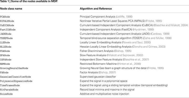
A node is the basic building block of an MDP application. It represents a data processing element, like for example a learning algorithm, a data filter, or a visualization step (see Table 1
for a list of some of the available algorithms). Each node is characterized by an input dimension (i.e., the dimensionality of the input vectors), an output dimension, and a
dtype, which determines the numerical type of the internal structures and of the output signal. By default, these attributes are inherited from the input data. Nodes can have a training phase, where training data is analyzed in order to adapt the internal variables, and an execution phase, where new data can be processed using the learned parameters. For example, the Principal Component Analysis (PCA) algorithm (Jolliffe, 1986
) requires the computation of the mean and covariance matrix of a set of training data from which the principal eigenvectors of the data distribution are estimated. MDP offers an implementation of this algorithm in the class
PCANode. The node can be trained on the data using the interface common to all nodes: PCANode.train(x) analyzes a new batch of data x, and updates the estimation of mean and covariance matrix; PCANode.stop_training() finalizes the algorithm by computing and selecting the principal eigenvectors. Once the training is finished, new data can be projected on the principal components calling the PCANode.execute(y) method. If the transformation specified by the underlying algorithm is invertible, the node can also be executed “backwards” using the PCANode.inverse(z) method. In the case of PCA, for example, this corresponds to projecting a vector in the principal components space back to the original data space.Node was designed to be applied to arbitrarily long sets of data: if the underlying algorithms support it, the internal structures can be updated incrementally by sending multiple batches of data. It is thus possible to perform computations on amounts of data that would not fit into memory or to generate data on-the-fly. The general form of the training phase thus is:# create an instance of the desired nodenode_instance = mdp.nodes.XXXNode()for data_batch in data_source:node_instance.train(data_batch)node_instance.stop_training()In the code,
data_source can be any Python iterator
5
(e.g. a list, an iterator object, or a generator function) that returns an array with a batch of training data. The last line finalizes the training phase. It is shown here for completeness, but can replaced by a call to the execute or inverse methods. Nodes also define some utility methods, like for example copy and save, that return an exact copy of a node and save it in a file, respectively. Additional methods may be present, depending on the algorithm. The PCANode.get_projmatrix method, for example, returns the matrix projecting input data into the principal components’ space. For a toy signal-denoising application that makes use of the basic Node features just described in Figure 1
.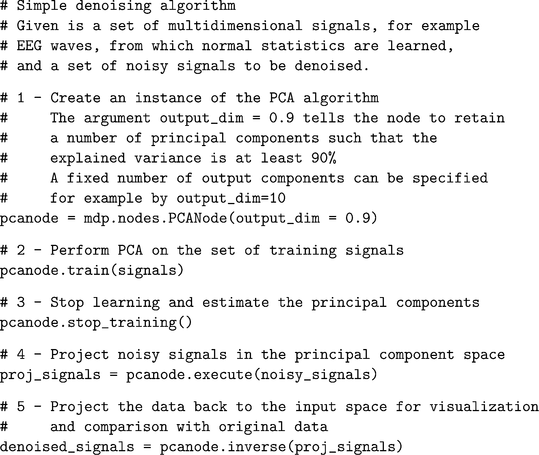
Figure 1. A simple denoising application.
Some nodes, namely the one corresponding to supervised algorithms, e.g. Fisher Discriminant Analysis (Bishop, 1995
), may need some labels or other supervised signals to be passed during training:
input = {‘a’: data_a, ‘b’:data_b, ‘c’:data_c}fdanode = mdp.nodes.FDANode()for label in [‘a’, ‘b’, ‘c’]:fdanode.train(input[label], label)A node could also require multiple training phases. For example, the training of
fdanode is not complete yet, since it has two training phases: The first one computing the mean of the data conditioned on the labels, and the second one computing the overall and within-class covariance matrices and solving the FDA problem. The first phase must be stopped and the second one trained:fdanode.stop_training()for label in [‘a’, ‘b’, ‘c’]:fdanode.train(input[label], label)The easiest way to train multiple phase nodes is using flows, which automatically handle multiple phases (see Flows).
MDP makes it easy to write new nodes that interface with the existing data processing elements. The
Node class is designed to make the implementation of new algorithms easy and intuitive. This base class takes care of setting input and output dimension and casting the data to match the numerical type (e.g. float or double) of the internal variables, and offers utility methods that can be used by the developer. To expand the MDP library of implemented nodes with user-made nodes, it is sufficient to subclass Node, overriding some of the methods according to the algorithm one wants to implement, typically the _train, _stop_training, and _execute methods. Figure 2
shows an example of a simple node that removes the mean of the signal. A more detailed introduction to writing new nodes in MDP can be found in the online tutorial
6
.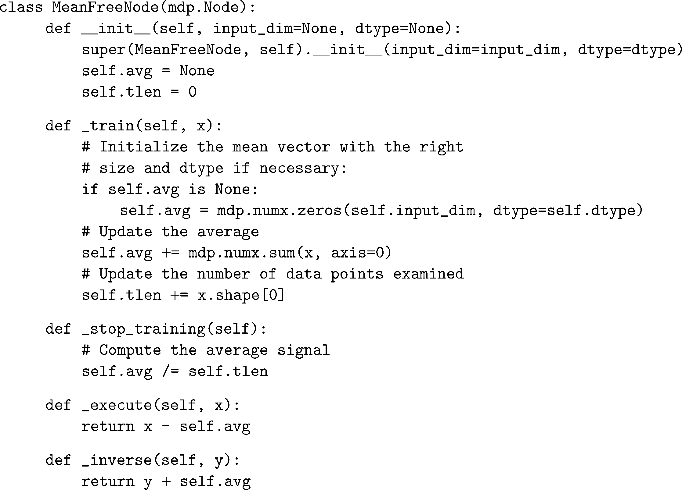
Figure 2. Definition of a new node that removes the mean of the signal.
It is also possible to specify multiple training phases by defining additional training methods and overwriting the
_get_train_seq method. For exampleclass MultiplePhaseNode(mdp.Node):def _get_train_seq(self):return [(self._train_A, self._stop_A),(self._train_B, self._stop_B)][...]defines a new node with two training phases, one updated by the method
_train_A and finalized using _stop_A, and analogously the second is defined by the methods _train_B and _stop_B. The final user will still perform the training phase by calling the usual methods train and stop_training (although multiple times), and need not know about the specific implementation of the algorithm.Flows
A flow is a sequence of nodes that are trained and executed together to form a more complex algorithm. Input data is sent to the first node and is successively processed by the subsequent nodes along the sequence. Using a flow as opposed to handling manually a set of nodes has a clear advantage: The general flow implementation automates the training (including supervised training and multiple training phases), execution, and inverse execution (if defined) of the whole sequence. For example, suppose we need to analyze a very high-dimensional input signal using Independent Component Analysis (ICA). To reduce the computational load, we would like to reduce the input dimensionality of the data using PCA. Moreover, we would like to find the data that produces local maxima in the output of the ICA components on a new test set (this information could be used for instance to characterize the ICA filters). To implement this algorithm using MDP, we need to generate an instance of
Flow using the appropriate nodes:# Define a data processing sequence.# - PCANode(output_dim=5) performs PCA and keeps# the first 5 principal# components only# - CuBICANode() is a cumulant-based ICA algorithm# - HitParadeNode(3) records the 3 largest local# maxima from the output of# the previous nodeflow = mdp.Flow([mdp.nodes.PCANode(output_dim=5),mdp.nodes.CuBICANode(),mdp.nodes.HitParadeNode(3)])The training and execution are performed as for the
Node class:# Train all the nodes using the data array ‘x’flow.train(x)# Compute the output of the node sequence# when presented with array ‘x_test’output = flow.execute(x_test)A single call to the flow’s
train method will automatically take care of training nodes with multiple training phases, if such nodes are present.Flow objects are defined as Python containers, and thus are endowed with most of the methods of Python lists: one can obtain slices, append new nodes, pop or insert nodes, and concatenate flows. For example, to get the maxima computed by the HitParadeNode, one can refer to the last node using the list construct flow[-1]:maxima, indices = flow[-1].get_maxima()The
Flow class defines a number of utility methods, including save and copy methods. It also implements a crash recovery mechanism that can be activated by setting a flag: in case an exception is thrown during training, the current state of the flow is saved for later inspection.Hierarchical Networks
In case the desired data processing application cannot be defined as a sequence of nodes, the
hinet subpackage makes it possible to construct arbitrary feed-forward architectures, and in particular hierarchical networks. It contains three basic building blocks (which are all nodes themselves): Layer, FlowNode, and Switchboard.The first building block,
Layer, works like a horizontal version of flow. It acts as a wrapper for a set of nodes that are trained and executed in parallel. For example, we can combine two nodes with 100-dimensional input to construct a layer with a 200-dimensional input:node1 = mdp.nodes.PCANode(input_dim=100, output_dim=10)node2 = mdp.nodes.SFANode(input_dim=100, output_dim=20)layer = mdp.hinet.Layer([node1, node2])The first half of the 200-dimensional input data is then automatically assigned to
node1 and the second half to node2. We can train and execute a layer just like any other node. In order to be able to build arbitrary feed-forward node structures, hinet provides a wrapper class for flows (i.e., vertical stacks of nodes) called FlowNode. For example, we can replace node1 in the above example with a FlowNode:node1_1 = mdp.nodes.PCANode(input_dim=100, output_dim=50)node1_2 = mdp.nodes.SFANode(input_dim=50,output_dim=10)node1_flow = mdp.Flow([node1_1, node1_2])node1 = mdp.hinet.FlowNode(node1_flow)node2 = mdp.nodes.SFANode(input_dim=100,output_dim=20)layer = mdp.hinet.Layer([node1, node2])node1 has two training phases in this example, one for each internal node. Therefore layer now has two training phases as well and behaves like any other node with two training phases. By combining and nesting FlowNode and Layer, it is thus possible to build complex node structures.When implementing networks one might have to route different parts of the data to different nodes in a layer in complex ways. This is done by the
Switchboard node, which can handle such routing. A Switchboard is initialized with a 1-dimensional array with one entry for each output connection, containing the corresponding index of the input connection that it receives its input from, e.g.:switchboard = mdp.hinet.Switchboard(input_dim=6, connections=[0,1,2,3,4,3,4,5])print switchboard# should print: Switchboard(input_dim=6,# output_dim=8,# dtype=None)x = mdp.numx.array([[2,4,6,8,10,12]])print switchboard.execute(x)# should print: # array([[ 2, 4, 6, 8, 10, 8, 10, 12]])The switchboard can then be followed by a layer that splits the routed input to the appropriate nodes, as illustrated in Figure 3
.
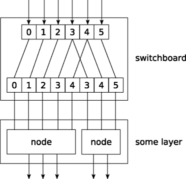
Figure 3. Example of feed-forward network topology.
Since hierarchical networks can become quite complicated to build and debug,
hinet includes the class HiNetHTML that translates an MDP flow into a graphical visualization in an HTML file.In this section we show a complete example of MDP usage in a machine learning application, and use non-linear Slow Feature Analysis for processing of non-stationary time series. We consider a chaotic time series derived by a logistic map (a demographic model of the population biomass of species in the presence of limiting factors such as food supply or disease) that is non-stationary in the sense that the underlying parameter is not fixed but is varying smoothly in time. The goal is to extract the slowly varying parameter that is hidden in the observed time series. This example reproduces some of the results reported in Wiskott (2003)
. The complete code is shown in Figure 4
.
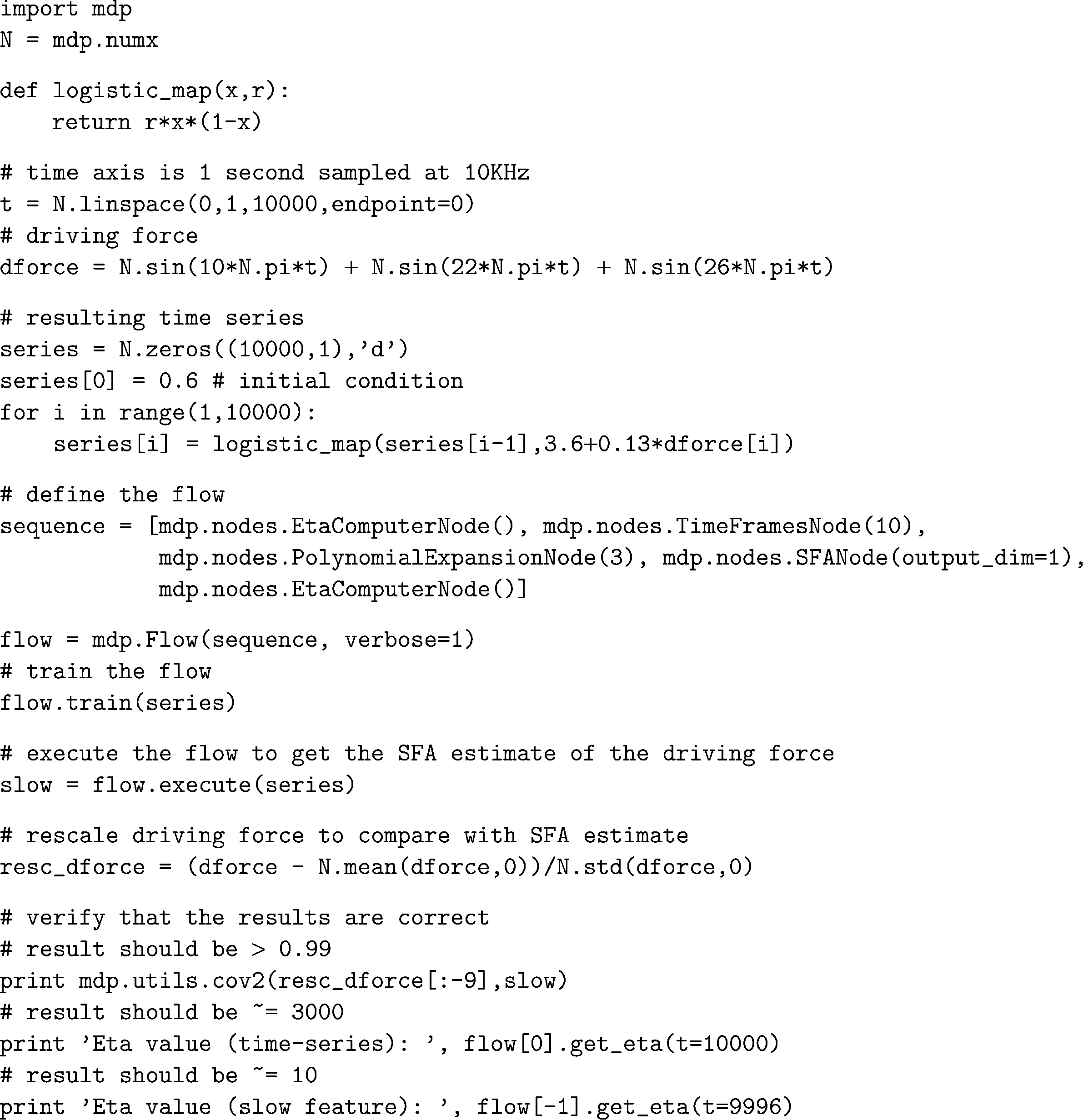
Figure 4. Python code to reproduce the results in Wiskott (2003).
We first generate the slowly varying driving force parameter rt as a combination of three sine waves rt = sin(10πt) + sin(22πt) + sin(26πt). We then generate the time series using the logistic equation xt +1 = (3.6 + 0.13rt)xt (1 − xt). The resulting time series x is shown in Figure 5
.
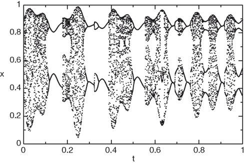
Figure 5. Chaotic time series generated by the logistic equation.
To reconstruct the underlying parameter, we define a
Flow to perform SFA in the space of polynomials of degree 3. We first use a node that embeds the 1-dimensional time series in a 10-dimensional space using a sliding temporal window of size 10 (TimeFramesNode). Second, we expand the signal in the space of polynomials of degree 3 using a PolynomialExpansionNode. Finally, we perform SFA on the expanded signal and keep the slowest feature using the SFANode. In order to measure the slowness of the input time series before and after processing, we put at the beginning and at the end of the node sequence a node that computes the η-value (a measure of slowness, see Wiskott and Sejnowski, 2002
) of its input (EtaComputerNode). The slow feature should match the driving force up to a scaling factor, a constant offset and the sign. To allow a direct comparison we rescale the driving force to have zero mean and unit variance. The real driving force is plotted together with the driving force estimated by SFA in Figure 6
.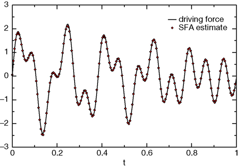
Figure 6. The real driving force and the driving force as estimated by SFA.
MDP is currently maintained by a core team of three developers, but it is open to user contributions. Users have already contributed some of the nodes, and more contributions are currently being reviewed for inclusion in future releases of the package. The package development can be followed on the public subversion code repository
7
. Questions, bug reports, and feature requests are typically handled by the user mailing list
8
.
Development of the core functionality of MDP continues and the next release of MDP is going to include a new package for parallelization, designed for nodes in which a large part of the computation is embarrassingly parallel
9
(e.g. calculating the covariance matrix to perform PCA). The new parallel package will consist of two parts: The first part introduces parallel versions of the familiar MDP structures (nodes and flows, including
hinet) that are able to split the computations for some of the algorithms (e.g. PCA and SFA). The second part of the package consists of schedulers that take individual jobs and execute them in a parallel way. Currently a scheduler for parallelization across multiple processors (or cores) is provided. Since the scheduler code is largely independent of MDP, one can write simple adapters for other schedulers like for example Parallel Python
10
. The new parallel subpackage can be tested already and it is available on the public code repository.Another new, large MDP package is currently under development that will extend MDP with more complex data flows, including back-propagation and loops. This framework will be integrated with both the parallel and the
hinet package to allow for large and complex data processing networks.MDP could also act efficiently as a wrapper for the plethora of statistical data analysis algorithms already available in other libraries and languages. A prominent example is the R Project for Statistical Computing
11
with the Python wrappers RPy
12
and R/S Plus
13
.
With over 10,000 downloads since its first public release in 2004, MDP has become one of Python’s major scientific packages. The package has minimal dependencies, requiring only the NumPy numerical extension, is completely platform-independent, and is available in the Linux Debian distribution and the Python(x,y)
14
scientific Python distribution.
MDP has been used to implement a model of the visual system of a virtual rat moving around in a virtual environment (Franzius et al., 2007
), to perform pattern recognition (Franzius et al., 2008
) and handwritten digit recognition (Berkes, 2006
), to analyze intra-cerebral array-recorded neurophysiological data in the auditory forebrain of song birds
15
, and to perform PCA and spike-sorting of electrophysiological data (Wiltschko et al., 2008
), to name a few of the applications in computational neuroscience. MDP has also been used embedded in the X-ray fluorescence mapping package PyMCA (Solé et al., 2007
), to implement auto tagging capabilities into the personal organizer application Chandler
16
by OSAF
17
, and as a framework for the implementation of data processing algorithms in the context of an advanced course in scientific computing (Zito and Wilson, 2008
) aimed at graduate students.
As the number of its users and contributors is increasing, MDP appears to be a good candidate for becoming a community-driven common repository of user-supplied, freely available, Python implemented data processing algorithms.
The authors declare that the research was conducted in the absence of any commercial or financial relationships that could be construed as a potential conflict of interest.
We wish to heartily thank Mathias Franzius for discussion and help during the early phases of the project, for being our main beta-tester afterwards, and for his code contributions. For contributing code and comments we thank Gabriel Beckers, Farzad Farkhooi, Susanne Lezius, Michael Schmuker, and Jake VanderPlas. For maintaining the Debian package we are grateful to Yaroslav Halchenko. We finally wish to acknowledge all those users who reported bugs and feature requests, which helped us making MDP a better library.
- ^ http://numpy.scipy.org
- ^ http://www.scipy.org
- ^ http://www.mathworks.com/products/matlab/
- ^ http://mdp-toolkit.sourceforge.net
- ^ http://docs.python.org/lib/typeiter.html
- ^ http://mdp-toolkit.sourceforge.net/tutorial.html
- ^ http://mdp-toolkit.svn.sourceforge.net
- ^ http://sourceforge.net/mail/?group_id = 116959
- ^ In the jargon of parallel computing, an embarrassingly parallel problem is one for which no particular effort is needed to segment the problem into a very large number of parallel tasks, that can be executed more or less independently, without communication among tasks (Foster, 1995 , Section 1.4.4.).
- ^ http://www.parallelpython.com
- ^ http://www.r-project.org/
- ^ http://rpy.sourceforge.net/
- ^ http://www.omegahat.org/RSPython/
- ^ http://www.pythonxy.com
- ^ Gabriel J.L. Beckers, Max Planck Institute for Ornithology, Starnberg, Germany, personal communication.
- ^ http://chandlerproject.org/
- ^ http://www.osafoundation.org/
Berkes, P. (2006). Temporal Slowness as an Unsupervised Learning Principle. Ph.D. Thesis, Humboldt-Universität zu Berlin, Mathematisch-Naturwissenschaftliche Fakultät I, http://edoc.hu-berlin.de/docviews/abstract.php?id = 26704
.
Franzius, M., Wilbert, N., and Wiskott, L. (2008). Invariant object recognition with slow feature analysis. In Proceeding of the 18th International Conference on Artificial Neural Networks (ICANN 2008), Prague, Czech Republic, September 3–6, 2008. Lecture Notes in Computer Science Series, Part I, Vol. 5163 (Berlin, Springer Verlag). http://www.springerlink.com/content/v20024g580t1/
.
Wiskott, L. (2003). Estimating Driving Forces of Nonstationary Time Series with Slow Feature Analysis. arXiv.org e-Print archive, http://arxiv.org/abs/cond-mat/0312317/
.
Zito, T., and Wilson, G. (2008). Software Carpentry for Scientists. http://itb.biologie.hu-berlin.de/∼zito/teaching/SC/
.