1
Max-Planck-Institute of Neurobiology, Martinsried, Germany
2
Faculty for Informatics, Technical University of Munich, Garching, Germany
Neuroscience is witnessing increasing knowledge about the anatomy and electrophysiological properties of neurons and their connectivity, leading to an ever increasing computational complexity of neural simulations. At the same time, a rather radical change in personal computer technology emerges with the establishment of multi-cores: high-density, explicitly parallel processor architectures for both high performance as well as standard desktop computers. This work introduces strategies for the parallelization of biophysically realistic neural simulations based on the compartmental modeling technique and results of such an implementation, with a strong focus on multi-core architectures and automation, i.e. user-transparent load balancing.
With neurobiology and biochemistry advancing steadily, biophysically realistic modeling has become an indispensable tool for understanding neural mechanisms such as signal propagation and information processing in both single neurons and neural networks. The high computational complexity of such neural simulations due to detailed models of ion channels and synapses, combined with high spatial resolutions of neuronal morphology, often result in long run times or require the use of a whole network of computers (a computer cluster).
The evolution of multi-cores, a new processor architecture in personal computer technology where several standard processing units are combined on one chip, providing the user with a multiple of the previous available computational power, has the potential to overcome these limitations. Moreover, multi-cores are likely to replace the current single-core processors completely in the future; as of today, most computers are available with dual-core or quad-core processors, only.
However, exploiting the potential of multi-cores requires manual adaptation of the algorithms and the source code. This, in turn, requires thorough knowledge of the internals of these chips, careful examination and parallelization of the algorithms used and extensive measurements to ensure the applicability of the parallelized program to a wide range of models.
This work introduces techniques for the parallelization of biophysically realistic neural simulations in a shared memory environment (i.e., where the processing units access a common main memory) using multithreading with a special focus on the characteristics of multi-core architectures.
Setting up the system of equations usually takes much more time than solving the equations, and parallel solving is algorithmically demanding; we therefore mainly focus on setting up the equations in parallel. Here, care must be taken to avoid workload imbalances due to different computational complexities of different types of transmembrane currents as well as their irregular distribution across a neuron. We propose two methods dealing with this issue. For solving, we use the comparatively simple, previously published splitcell method (Hines et al., 2008a
) for splitting neurons into subtrees and extend the method to automatically identify a split compartment and distribute the workload for solving of these subtrees onto processors in a balanced way.
The next section will give a short introduction to parallel programming, multi-core architectures and multithreading. The section on “Compartmental Modeling” contains a summary of the compartmental modeling technique and the splitcell method. The section on “Details about the Sample Implementation” describes the sample simulator software we implemented to test our algorithms. The algorithms themselves are presented in detail in the subsequent section, “Parallelized Simulations”. This part of the manuscript also contains a subsection comparing our approaches to previous neural simulator algorithms. The section “Results” presents performance results obtained with our sample implementation for models of varying complexity and memory requirements, followed by a discussion section summarizing the work and giving a short outlook.
In the last 40 years, processor manufacturers increased performance mainly by a) creating faster and smaller transistors and circuits allowing for higher clock frequencies, and by b) automatically exploiting parallelism inherent in the sequence of incoming instructions using overlapping and out-of-order execution. With the limited amount of instruction level parallelism in a sequential program and physical restrictions on the speed of transistors and electric signals traveling through a circuit, recent developments focus on providing multiple, user-visible processing units (PUs, also called cores). In the last few years, a new kind of architecture referred to as multi-cores emerged: Decreasing transistor sizes and improving manufacturing technologies are exploited to put multiple, full-blown PUs onto one chip. To exploit the computational capacities of this architecture, programs must be explicitly designed to make use of the available processing resources by first analyzing their algorithms for potential parallelism, followed by writing new or modifying existing source code that identifies workload distributions and subsequently assigns jobs to the available cores
1
.
General Rules for Parallelization
Computer clusters and single computers with multiple processing chips or multi-cores all require adapting the algorithms and code to make use of the available processing resources. Parallel code must strive to meet the following requirements:
• The time spent on sequential, i.e. non-parallel, regions of the code must be minimized.
• The work must be distributed across the PUs in a manner as balanced as possible.
• Overhead due to parallelization must be minimized. This includes overhead for initialization routines and synchronization operations.
Before continuing, two frequently used synchronization operations, mutexes and barriers, are introduced.
Mutexes (derived from mutual exclusion algorithm, also referred to as locks) are used to prevent the concurrent execution by different processes (running instance of a program) of specific parts of the code (or, thereby, the concurrent access to common data). A lock can be held by one process at a time only; processes trying to acquire a lock must wait until the lock is released by the process currently holding the lock.
In contrast, barriers are special functions that, once called, only return when all other processes have called the function as well. They are used to make sure all processes have reached a certain point in the program.
Both mutexes and barriers are indispensable methods in parallel programming. However, they come at the cost of inter-process communication; depending on how big the latency of the interconnection technology is, they can influence the runtime significantly if not used with caution. In typical message-passing environments (see Programming Multi-Cores) where inter-process communication usually requires sending messages across a network from one computer to another, latencies for small messages range between about 4 μs (InfiniBand, see Liu et al., 2005
) and 30 μs (Ethernet, see Graham et al., 2005
). Thus, synchronization operations quickly become a bottleneck. It is therefore necessary to reduce such communication as far as possible, i.e. let the processes compute independently as long as possible.
In contrast, inter-core communication on multi-cores is extremely fast (see next section) and allows for much finer-grained parallelization, i.e. the efficient parallel computation even of small problems where synchronization operations are frequent. Still, synchronizations come at a certain cost and can have a significant effect on runtime if used extensively.
Multi-Core Characteristics
In some architectures, different types of PUs are combined on one chip, e.g. IBM’s Cell Broadband Engine Architecture (Johns and Brokenshire, 2007
). However, the most widespread type are homogeneous multi-core architectures where multiple copies of the same PU are placed on a single chip, e.g. Intel’s Core 2 Duo processors (Intel Corp., 2006
), AMD’s Opteron K10 series (AMD, Inc., 2007a
) or IBM’s POWER5 dual-cores (Sinharoy et al., 2005
). This work will focus on the latter architecture, although most concepts derived in this work are applicable to heterogeneous multi-core architectures as well.
Before going into further detail, a note about caches must be made because they play a very important role in developing software for multi-cores. In the context of processors, a cache refers to a very fast (compared to main memory) on-chip memory where previously accessed data from main memory is temporarily stored to reduce the latency of subsequent memory read and write accesses. A good way to ensure cache-efficiency is to layout data in main memory both in a packed way and in the sequence of program accesses. This allows the processor to perform so-called prefetching of data when it realizes the program traverses an array.
The use of multiple caches requires a mechanism referred to as cache-coherency protocol to ensure integrity when different cores access the same location in main memory. Depending on what type of cache-coherency protocol is used, communication between cores that share a cache may be much faster than between cores that access separate caches (explained later in this section).
Figure 1
opposes a single-core processor with memory and I/O controllers attached via the front side bus (FSB) to two modern quad-core processors, Intel’s Xeon X5355 and AMD’s Opteron K10 2347. Three important characteristics of homogeneous multi-core processors and consequences arising therefrom can be observed:
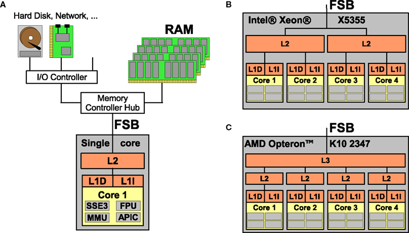
Figure 1. (A) Processor with a single core featuring Level 1 instruction and data caches (L1I and L1D), Level 2 cache (L2), and main memory (RAM) accessed via the Front Side Bus (FSB); the core is equipped with subunits for e.g. vector arithmetics, floating point processing, memory management and an interrupt controller. (B) A multi-core processor with four cores where two cores share a L2 cache, respectively. (C) A multi-core processor where all cores have a private L2 cache but a L3 cache shared between all four cores.
• All cores are full-blown copies of a single-core’s PU; this makes programming for multi-cores a comparatively simple task because a single program can be used on all four cores, and porting existing applications is simple from a programmer’s point of view.
• All cores on a chip share external resources like main memory, main memory bandwidth as well as processor-external hardware and hardware bandwidth (network controllers, hard disk drives etc.). While the access to shared resources simplifies programming and allows for fast interaction between the cores, it also bounds the efficiency of parallel programs that require a high memory or I/O bandwidth and low latency for every core.
• Inter-core communication is very fast compared with computer clusters where latencies range between 4 and 30 μs. The latency of inter-core communication strongly depends on whether cores share a cache or not and the exact cache-coherency protocol used.
For instance, the inter-core latency on Intel’s Xeon X5355 can be as low as 26 ns if two cores communicate via a shared cache but is much higher if the two cores do not share a cache (between 500 and 600 ns depending on whether the two cores are on the same or on different chips) because communication is performed by exchanging data via the comparatively slow main memory (Intel Corp., 2007
). In contrast, on AMD’s Opteron K10 2347, the set of cores used does not influence the inter-core latency significantly; on our test system, we measured latencies of 240 and 260 ns for two cores sharing a cache or not, respectively. This is because AMD processors use a different way for ensuring cache coherency (AMD, Inc., 2007b
) where cores can communicate directly without accessing main memory even if they are located on different chips.
The main intention of this work is to evaluate, in the context of neural simulations, how the advantages of multi-core architectures can be exploited and when their limitations influence efficiency. This requires mentioning another computer architecture first, symmetric multi-processing (SMP). Here, multiple processor chips (possibly multi-core chips) are combined in one computer in a manner similar to how cores are combined on a multi-core chip. The main differences are a) that multi-cores are becoming ubiquitous devices, while SMP systems never saw widespread use except for some scientific areas and in servers, b) that cores on the same chip can communicate much faster, and c) that the number of processors/chips in one SMP system is low (usually two, seldom more than four) while multi-core chips are likely to comprise up to 32 or more cores on a chip in the near future. Therefore, albeit there are no differences between these two architectures from a programmer’s point of view, the higher number of cores and the low inter-core communication latency pose new scalability requirements, while at the same time allowing for finer grained parallelization strategies. Nevertheless, the principles derived in this work are applicable to SMP systems as well.
Programming Multi-Cores
Parallel programming paradigms can be divided into two classes, message-passing and shared memory programming. In message-passing, every process accesses its own memory region and communicates with other processes by explicitly sending and receiving messages. This is the standard programming model for all kinds of computer clusters but is also frequently used on hybrid architectures (networks of multiprocessor systems) or even on shared memory systems.
Shared memory programming, on the other hand, is based on processes communicating with each other by accessing common physical memory regions to change and read shared variables. This model can take various forms, for instance two different programs that share a small region of memory to exchange information. The most common method of shared memory programming in scientific computing is multithreading; here, multiple instances of the same program, so called threads, are executed in parallel, all residing in the same memory space (i.e. sharing all memory regions
2
), although different threads may be at different points in the program at one time.
This paper user multithreading for two reasons. First, it is a standard method for concurrent programming on desktop computers and is available on most modern operating systems without requiring the installation of additional libraries. Second, using multithreading instead of message-passing for compartmental model simulations is a rather novel approach that deserves exploration. The exact method is a slight modification of the Fork&Join model, e.g. used by OpenMP (OpenMP Architecture Review Board, 2002
). The program is executed in a single-threaded manner, except for parallel regions of the code, where the first thread invokes other threads to take part in the parallel computation of this region.
The next section will introduce the mathematical and algorithmic basis of most types of realistic neural simulations, compartmental modeling.
This work focuses on a popular technique in neural simulations: compartmental modeling based on an electric equivalent circuit of a neuron. There, a neuron’s morphology is represented by a set of cylinders of different length and diameter, so-called compartments, that are electrically coupled with axial conductances. The accuracy of this spatial discretization method depends solely on the user’s requirements; cells can be modeled with only one compartment or in a highly detailed fashion using up to tens of thousands of compartments; also, different regions of a cell may be modeled with varying precision.
Figure 2
A depicts the compartmental representation of a VS1 cell from the blowfly’s visual system, reconstructed from a cobalt-filled cell (Borst and Haag, 1996
).
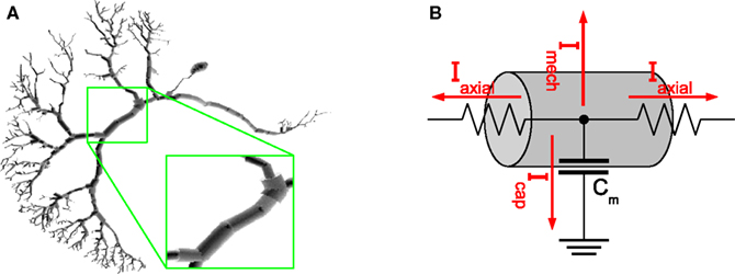
Figure 2. (A) Compartmental model of a VS1 cell from the blowfly’s visual system. The magnification inset emphasizes how cylinders are used to model the cell. (B) Example of an electric equivalent circuit used to simulate a compartment. The circuit in the picture is the one used by NEURON.
Ion channels, ion pumps, synapses and membrane capacitance are all modeled with electric equivalent circuits that aim to imitate the real behavior as good as possible or computationally feasible. Figure 2
B shows how a single compartment is represented by a circuit comprising axial currents Iaxial, capacitive currents Icap, and a current Imech modeling the sum of various neural mechanisms such as ion channels and pumps, chemical synapses and gap junctions
3
, and voltage or current clamps. For every compartment i with adjacent compartments j ∈ adji and directed currents as illustrated in Figure 2
B, this results in a current balance equation,
yielding
The set of all equations representing the compartmental model of a neuron forms a system of coupled ordinary differential equations, one for every compartment. Such systems are solved by applying a temporal discretization scheme, for instance forward Euler, backward Euler or Runge–Kutta methods, to every equation. The simulation is then carried out by starting at t = 0 and advancing in time step by step, i.e. from time t to t + Δt to t + 2Δt and so on. For every time step t → t + Δt, the neural simulation software sets up all equations based on voltages V(t), rate variables etc. defined at time t and solves the system for V(t + Δt).
Depending on the temporal discretization method used, solving the system for the new membrane potentials requires either a matrix-vector multiplication and a vector-vector addition, only (explicit methods), or a linear system of equations (LSE) must be solved (implicit methods). This work will focus on implicit methods because parallelization is rather simple for explicit methods and because implicit methods provide a higher degree of numerical stability which is often crucial for neural simulations. When using an implicit method such as the backward Euler method,
which is also NEURON’s default method, and applying an approximation to the mechanism terms (for details, see Section 4.3 and Appendix A in Eichner, 2007
or pp. 168–169 in Carnevale and Hines, 2006
), the equations can be rewritten in matrix-vector form with some right-hand side term rhs as

Figure 3
A shows a numbered graph whose circles represent compartments, while the lines represent electrical couplings between the compartments. The corresponding layout of G is illustrated in Figure 3
B, where X denotes non-zero entries. G can thus be seen as the adjacency matrix of the underlying, tree shaped neuron.
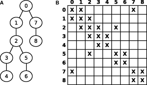
Figure 3. (A) Numbered graph representing a set of connected compartments. (B) Layout of the corresponding matrix G.
For n compartments, G ∈ Rn×n is a sparse matrix with all elements being zero except for about 3n elements, namely diagonal elements (i,i) and off-diagonal elements at (i,j) and (j,i) for two axially connected compartments i and j; i.e., the matrix layout reflects the connectivity structure of the model. For example, an unbranched cable yields a strictly tridiagonal matrix G. Hines (1984)
discovered that solving LSEs corresponding to tree structured grids can be performed such that the required time is linear in the number of compartments [O(n), as opposed to the usual complexity of O(n3)] if they are numbered in a special way and the solver algorithm exploits the sparse structure of the resulting matrix.
In short, the compartments are numbered increasingly using depth-first search, starting with 0 at some arbitrarily chosen root compartment. Then, Gaussian elimination requires only O(n) non-zero elements above the diagonal to be eliminated (fill-in does not occur) instead of the usual O(n2), and the sparse structure allows to reduce the weighted addition of two rows required for elimination to the weighted addition of only two floating point values. The complexity of back-substitution, usually O(n2), can also be reduced to O(n) because the number of left-diagonal elements in every row is limited to one.
A closer look at the data dependencies of Gaussian elimination reveals that there are several possibilities in what order the compartments may be processed (i.e., in what order above-diagonal elements are eliminated). While one might start with compartment 8, proceeding with compartment 7, 6 and so on, another possibility is to process compartments 4, 3, 6 and 5, then proceed with compartment 2 etc. The governing rule is that a compartment may only be processed once all subordinate compartments in leaf direction have been processed. The same applies, with inverse data dependencies, to back-substitution.
This observation is visualized in Figure 4
. Part A shows the data dependency graph for Gaussian elimination, while part B depicts the data dependency graph for the back-substitution algorithm. Although the data-dependencies impose some restrictions on the order of how compartments are processed, there is nonetheless a certain degree of freedom in choosing a sequence of compartments during Gaussian elimination or back-substitution. Again, the choice of the root compartment (and thus the exact data dependency graph) is left to the programmer. These observations will play an important part in parallelizing Gaussian elimination. For a more detailed explanation of these findings, see Eichner (2007)
. Iterative methods for solving the LSE such as Gauss-Seidl or conjugate gradients (Hestenes and Stiefel, 1952
) are not considered because of the superior performance of Hines method.
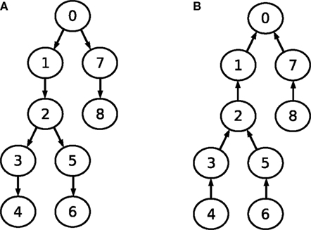
Figure 4. Data dependency graphs for (A) Gaussian elimination and (B) back-substitution of an LSE with a matrix as depicted in Figure 3
.
We implemented our algorithms in a stand-alone application for Linux. The source code is based on the numerical core of NEURON (Carnevale and Hines, 1997, 2006
). Specifically, we re-implemented the fixed-step backward Euler scheme and ported a set of mechanisms to our application by modifying the C source code generated by NEURON’s
nrnivmodl to suit our needs. The program is missing a user interface; it runs simulations by reading in a configuration file that contains the matrix and information about what mechanisms are used on what compartments and mechanism specific parameters. This configuration file completely describes the model and can be generated by an arbitrary frontend. As we wanted to simulate existing NEURON models and reproduce the results, we patched NEURON 6.0 such that it generates the configuration file upon initializing a model; the file is then used by our application to perform the simulation.We checked the validity of our results by printing the voltage at every time step for every 100th compartment and comparing it to the corresponding value NEURON computes. The results never deviate more than 1 μV from NEURON’s results for the same model; in most cases, the deviations are smaller than 0.001 μV
4
.
The program uses the Native POSIX Thread Library implementation (Drepper and Molnar, 2005
) of the POSIX threads standard (IEEE Portable Applications Standards Committee, The Open Group, ISO/IEC Joint Technical Committee 1 2004
) for managing threads and synchronizations. Additional threads are created by the first thread in an initialization function and invoked when parallel regions are encountered. Then, the threads are notified of the code and the data they must process.
One important technical aspect is how inter-core communication for notifying or waiting for other threads is implemented. Threads can wait passively by relinquishing their processor to the operating system, waiting to be invoked again at some later point in time when a signal from another thread arrives. The other alternative is to wait actively by spin-waiting on some shared variable to be changed by another thread. While the passive waiting method is fairer because the processor is only utilized when anything useful is computed, it bears a certain overhead due to the invocation of the operating system. In contrast, the active waiting method is much faster but fully occupies the processor even when no actual computation is performed. When the relative importance of the notification method is high, i.e. for small models, the operating system visible method becomes ineffective. We implemented and benchmarked both methods but decided to only show results obtained with the spin-waiting method. In summary, both methods give identical performance for larger models but spin-waiting is much more effective for smaller models. The implementation’s source code, the configuration files used in this paper, the result files and corresponding documentation for building and running the program are freely available from http://fneuron-mc.myselph.de
.
In most neural simulations, setting up the equations and computing the actual conductances as a result of the previous voltage distribution takes up the majority of the time. Our experience is that about 40% of the time is spent on equation setup when only a passive mechanism is used, while additional active membrane mechanisms increase this value to between 80–95% or even more. Fortunately, it is rather simple to gain proper parallel performance for mechanism setup. At the same time, parallelizing the equation solver is difficult from both an algorithmic and from a programmer’s point of view, while the influence on the performance of the program is usually rather small.
Therefore, this work will focus on parallel equation setup first without considering solving the equations. Then, a simple but effective algorithm for parallel solving of single cells and networks of cells is presented.
Although handling equation setup and solving as independent tasks seems like an obvious choice, this is nonetheless one of the main novelties presented in this paper which was not employed by previous approaches to parallel neural simulations; it will be compared to existing techniques in the section “Comparison to Existing Approaches”.
Parallel Equation Setup
While the setup of an equation consists of computing capacitive and axial terms as well, it is the calculation of transmembrane currents of all kinds modeled by mechanisms that is responsible for the majority of the runtime spent on this compartment. To simplify the following considerations, two terms must be introduced. A mechanism or mechanism type comprises the code used for computation of the transmembrane current contributions of this mechanism. A mechanism instance is the result of an instantiation of a mechanism type for a specific compartment, encapsulating the data this mechanism needs to compute its current contribution to this compartment.
The transmembrane current for compartment i is a combination of the capacitive current CmVi and the contribution of all mechanism instances mechsi on this compartment:
Mechanism types range from fairly simple mechanisms like the linear model for passive ion channels to complex and therefore computationally intensive mechanism types for ionic currents with the conductance governed by voltage- or ion-concentration dependent first-order kinetics, or models for synaptic mechanisms with highly detailed models of both transmitter release and postsynaptic ion channel kinetics. In particular, the kind and the location of mechanisms used in a model depend on the user’s requirements of accuracy as well as the knowledge about the modeled cell’s electrophysiological properties.
The number and the complexity of mechanisms used on a specific compartment are model-specific; while the blowfly’s HS network simulated in the section “Automatic Cell Splitting and Distribution” uses passive ion channels only, the more elaborate CA1 pyramidal cell model in the section “Mechanism Computation” uses up to six mechanism types per compartment for different kinds of ion channels. Whether parallel execution is worthwhile depends on several parameters such as the number of compartments, the number and the complexity of the involved mechanisms, and the number of threads and cache architecture used. We will approach this question in the “Results” section.
This work is based on the assumption that there are neither inter-compartmental nor intra-compartmental dependencies imposed upon mechanism computation, i.e. the order in which different mechanism instances on the same compartment or on different compartments are computed does not affect the result
5
. In other words, the contribution of a mechanism to a compartment’s transmembrane current may be computed in parallel to other mechanism currents on this or other compartments. Care must be taken when two mechanism instances on the same compartment are computed by different cores, however. While the computation itself can be performed in parallel, synchronizations must be used at some point to prevent the concurrent modification of the equation by these cores.
This leaves many possibilities for distributing mechanism instance computation onto the available cores; however, several constraints must be taken into account:
(1) Different mechanisms are often used on different sets of compartments, e.g. passive ion channels and synaptic mechanisms on dendritic compartments, active ion channels on somatic and axonal compartments.
(2) Different mechanism types have different computational requirements. Taking into account the first point as well, this means simply splitting up the set of compartments into equally large subsets for every core does not necessarily give a proper load balance.
(3) The overhead spent on synchronizations between cores for ensuring no equation is accessed concurrently by different cores must be minimized. Although inter-core communication as required for synchronizations is very fast on multi-cores, it can still lead to problems if used extensively. For instance, it is not feasible to use lock and unlock operations around every single write access of a mechanism to an equation.
(4) To avoid equation variables being transferred between different core’s caches, a compartment should be processed (i.e. computing its mechanism instances and solving its equation) by as few cores as possible (also, this reduces the amount of synchronizations).
Several techniques were evaluated and compared; the following two methods were found to account best for the mentioned restrictions.
Splitting up Mechanism Types
A very simple method that guarantees load balance is to split up the set of mechanism instances of every mechanism into ncores subsets that contain the same amount of compartments. Every core then computes its part of every mechanism instance set.
Two mechanism instance sets assigned to different cores may affect in part the same compartments; in particular, this results in the equations of some compartments being modified by two different cores, a possible source of concurrent write accesses. This problem is illustrated in Figure 5
. Here, some distribution of mechanism instances for different mechanism types across a compartmental model is shown. The hatching indicates to which of two cores the subset is assigned. For some compartments, the mechanism instances are computed by more than one core, e.g. some of the axonal compartments are processed by both the second and the first core. If the first core is ahead of the second core (e.g. because other running programs or hardware events interrupted the second core for some time), a situation may occur where the first core accesses an axonal compartment during the
passive mechanism computation which is at the same time accessed by the second core computing this compartment’s Active K instance. Similar conflicts could occur for the synaptic current computation in dendritic compartments.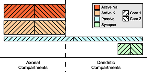
Figure 5. Mechanism type level parallelization. Height of mechanism type bars indicates per-compartment complexity. Distribution of different mechanisms (height indicates complexity) across the cell is often spatially inhomogeneous. Here, computation of the mechanism instances on one specific compartment is often performed by different cores and requires synchronizations after each mechanism type.
The simplest way to prevent such accesses is to perform a barrier operation after every mechanism type computation, illustrated in the pseudo code listing in Figure 6
. As the instances of a specific mechanism are distributed across the cores in a balanced manner, the time spent on waiting in the barrier function for other cores is usually very low. However, this overhead may still pose a problem when the model complexity per time step is rather low relative to the time spent on inter-core communication. This is the case for rather small models or models with a high amount of different mechanisms with only few instances each. The synchronization overhead could be mitigated by determining where conflicts can actually occur and only use barrier functions there (in Figure 5
: only after
Active K and Passive), but many models still require a high amount of synchronizations.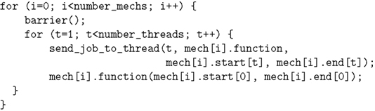
Figure 6. Pseudo-code listing for mechanism type level parallelization. The first thread waits for the other threads to be ready, then assigns them jobs in the form of a mechanism function and parameters that define the first and the last mechanism instance this thread must compute. Finally, the first thread calls the mechanism function itself.
A second possibility is to let the mechanisms store their computed values in extra arrays instead of adding them to the equations. Then, no synchronizations are needed between mechanism types, and the values are collected and added to the equations after all mechanism types have been computed. We implemented this method but found it to be inferior to the default method in the cases we tested, possibly due to the increased memory requirements.
Splitting up the Set of Compartments with Dynamic Load Balancing
Using synchronizations can be avoided in the first place if a compartment’s mechanism instances are all computed by one core only, i.e. the set of compartments is split up into ncores sets, and every core processes all mechanism instances on compartments in its set. The heterogeneity of mechanism complexity and mechanism distribution does not allow for simply splitting up the set of compartments into equally large consecutive subsets for each core, as one core might be assigned a computationally more demanding part of the cell than another core. Using non-consecutive subsets, e.g. distributing small subsets in a striped manner, would lead to cache-efficiency problems. The set of equations a core accesses during solving would be largely different from the set it accesses during equation setup, leading to a high amount of inter-core communication between the stages of setting up an equation and solving it, and vice-versa. What is needed is some estimate of the complexity of a compartment, so a distribution algorithm can calculate the size of consecutive compartment subsets assigned to a core.
Figure 7
shows how a balanced assignment of compartments to cores might look like. Although the set of compartments assigned to the first core is much smaller, the distribution of mechanisms across the cell makes this assignment the fairest in terms of mechanism complexity balance. No synchronizations are required because an equation is accessed by one core, only. The main question is how to identify these sets because the complexity of a mechanism is not known in advance.
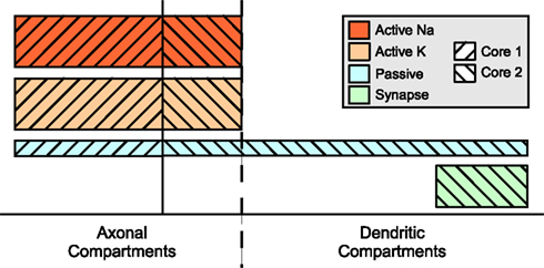
Figure 7. Compartment level parallelization. Solid line separates the two sets of compartments assigned to different cores. This boundary is chosen such that the overall complexity per core is very close to the average.
Hines et al. (2008a)
estimated a per-mechanism-type complexity before the actual simulation by performing a dummy simulation with 100 compartments for every mechanism type; mechanism complexity and mechanism distribution were then taken into account when distributing parts of cells onto nodes in a computer cluster. This requires additional simulations before the actual simulation and is only worth the overhead for longer simulations.
This work proposes a dynamic load balancing technique where the sets of compartments assigned to cores are resized during runtime to gain the best possible workload balance. After a fixed number of time steps, e.g. nsteps = 20, a per-mechanism-instance complexity mcm is estimated for every mechanism type m based on the accumulated time spent on this mechanism type on every core c, tm,c in the last nsteps timesteps and the number of mechanism instances of mechanism type m,  :
:
:
Following this, a per-compartment complexity coi is calculated for every compartment i based on the mechanism types mechsi used on this compartment:
When assigning only consecutively numbered compartments to a core, the first set of a out of ncomp compartments may then be determined by the following formula:
This technique has proven slightly superior to splitting up mechanism types (because of the missing synchronization operations) and significantly superior to simply splitting up the set of compartments without subsequent load-balancing (see Results). The technique is multithreading specific, i.e. it is not easily applicable to message-passing architectures such as computer clusters. Resizing sets during runtime is simple when the PUs share main memory because only loop indices must be changed; in message-passing environments, each PU has its own main memory, and resizing working sets requires parts of cells being loaded/unloaded during simulation and data such as voltages or rate variables must be sent to other PUs. This is possible in principle but difficult to implement, even more on top of an existing simulation program.
Parallel Equation Solving
Although equation solving usually represents only a small part of the overall runtime, it is nonetheless necessary to evaluate and exploit its parallel potential. First, there exist a significant number of models where compartments only with (computationally cheap) passive ion channels comprise the majority of the cell or even the whole model. Then, solving becomes a significant portion of the execution time. Second and more importantly, with the very good parallel performance of mechanism computation, equation solving would quickly become the time-limiting factor, especially for higher numbers of cores.
The following two sections will treat two ways of parallel solving, first how whole cells in a network of neurons, then how single cells may be solved in parallel. Finally, these two approaches will be combined in a simple algorithm which was found to deliver proper results in all models tested for this paper.
Whole Cell Balancing
In the section “Compartmental Modeling”, it was shown how the combination of equations for all compartments in a cell results in a system of coupled equations for every time step. Different cells may be seen as independent, i.e. not coupled, systems of equations. Although cells may be semantically connected by chemical synapses or gap junctions, these connections are modeled using mechanisms instead of off-diagonal elements in the connectivity matrix
6
. Thus, current flowing between two cells is accounted for during equation setup; solving the system of equations for different cells may be performed independently.
The complexity of solving the system of equations for a cell is linear in its number of compartments. Therefore, the resulting problem is to distribute the computation of solutions for n cells with different numbers of compartments onto ncores processing units such that the imbalance between cores is minimized; here, imbalance is defined as the difference between the two processing units with the highest and the lowest load. Although this appears to be a rather simple task at first glance, it is an NP-complete problem known as Number Partitioning Problem (Hayes, 2002
). This means that finding the solution requires checking an amount of cells-to-cores assignments increasing exponentially with the number of cells [O(ncoresn)]. Fortunately, heuristic algorithms with a much lower complexity exist that give reasonably good solutions.
The distribution algorithm used in this paper is very simple – the cells are first sorted in decreasing order according to their size (in compartments), then they are subsequently assigned to the core with the so far lowest number of compartments. Sophisticated algorithms like Karmarkar–Karp (Karmarkar and Karp, 1982
; Korf, 1997
) exist as well but were not tried because the performance reached by the above mentioned algorithm was found to deliver satisfactory load balance.
Whole-cell balancing has been employed frequently in parallel neural simulations, although not independently from equation setup (see “Comparison to Existing Approaches” for details). A much more interesting and challenging problem is to solve a single cell in parallel which is the focus of the next section.
Cell Splitting
It is important to once again emphasize that this work concentrates on the rather complex problem of parallelizing the process of solving LSEs. When explicit integration methods are used (which is the case for many simulators, e.g. the default in GENESIS), the system of equations may be solved by simply performing a matrix-vector multiplication, followed by a vector-vector addition, both tasks that are very efficient in parallel.
Implicit methods result in an LSE; solving LSEs in parallel has been a hot topic in research for a long time. In the special case of sparse matrices representing a tree-shaped connectivity structure, a method developed by Hines et al. (2008a)
allows for parallel solving of a cell by two PUs. This paper uses a similar, slightly enhanced version of this algorithm which is based on the following two facts. First, an arbitrary compartment may be chosen as the root compartment (see Compartmental Modeling). Second, subtrees of the root compartment may be solved in parallel, besides a synchronization operation between Gaussian elimination and back-substitution (see Figure 4
).
The main question is how to choose a root compartment given a specific neuron because this choice governs the number and size of the subtrees and thus the load balance achieved by splitting a cell. Most importantly, load balancing, including cell splitting, should be automated, i.e. require no user-interaction. The following algorithm is designed for the special case when only one cell is simulated; the case of parallel solving in networks of neurons is dealt with in the next section.
For single-cell simulations, the size of the largest subtree of the root compartment usually governs the load balance after distributing the single subtrees onto cores. Therefore, an algorithm that identifies the root compartment whose largest subtree is minimal among all possible root compartments seems to be a good solution. The algorithm presented here starts at an arbitrary compartment and traverses the tree by descending into the largest subtree of each visited compartment. It stops when the size of the largest subtree of the current compartment is lower than or equal to half of the overall number of compartments. This is the compartment whose largest subtree is smaller than or equal to all other compartments’ largest subtrees (a proof is given in Eichner, 2007
).
Figure 8
illustrates how an unnumbered graph (A) representing a neuron may be numbered such that the size of the largest subtree is minimal (B). The resulting subtrees (colored, part C) are then distributed onto the available cores with the same heuristic method that was introduced in the previous section for whole cell balancing. While Gaussian elimination may proceed simultaneously in the subtrees, all threads (at most three) must access the variables representing the root compartment’s equation, which is therefore not assigned to any core and not colored. This requires using mutexes for preventing concurrent write accesses to the root compartment’s equation and a barrier function to ensure every core has seen the changes of all other cores to that equation before using its values to continue with back-substitution.
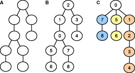
Figure 8. (A) Yet unnumbered tree-shaped graph representing the connectivity of some neuron. (B) Same graph, numbered such that the largest subtree connected to the root compartment (compartment 0) is as small as possible. (C) Same graph and numbering as for the middle graph, but restructured and colored to emphasize the distinct subtrees that may be solved in parallel.
Combining Cell Splitting and Whole Cell Balancing
A more common scenario is simulating more than just one cell. Trying to decide what cells to split and with what root compartment, i.e. sizes of subtrees, reveals several obstacles.
First, choosing a root compartment such that single cell Gaussian elimination is as efficient as possible may not be the best global choice, i.e. when taking all other cells and subsequent load balancing of whole cells and subtrees into account. Second, trees cannot simply be split such that the number of subtrees and the subtree sizes connected to the root compartment fulfill a certain requirement – even the rather simple constraint of choosing a root compartment such that its subtrees may be partitioned into two equally large sets often cannot be met as Figure 9
shows. Third, whole-cell balancing alone is NP-complete, so balancing subtrees and non-split whole cells is NP-complete as well.
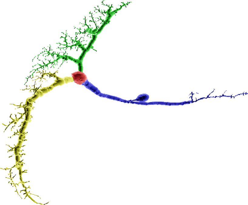
Figure 9. A VS2 cell’s compartmental model from the blowfly’s visual system (Borst and Haag, 1996
) split such that the largest subtree is minimized. Red indicates location of the root compartment. This cell cannot be split in a manner such that its subtrees can be partitioned into two equally large sets.
A heuristic approach seems reasonable that combines cell splitting and whole-cell balancing. The technique presented in this section is a combination of splitting neurons and distributing a number of neurons onto a set of processors. First, all cells are ordered according to their sizes. Then, the cells are split one after another, largest cell first, until the imbalance resulting from whole cell balancing of the subtrees of split cells and whole cells left is low enough, i.e. below a certain threshold. In our implementation, we use a maximal imbalance of 2% of the overall number of compartments. This method makes sure that unnecessary splitting of cells is avoided because every split cell results in additional synchronization overhead.
A more sophisticated method presented in Hines et al. (2008a)
computed a large set of possible root compartments for every cell along with the sizes of the connected subtrees and an estimate of their mechanism-dependent complexity in advance and made use of this information to split and distribute subtrees to PUs. This method requires considerable overhead as well as a mechanism-complexity estimate before the actual simulation is started. Most importantly, this method is designed for message-passing architectures where both dynamic load balancing is very difficult and the load balance achieved plays a much more important role as the net section will show.
The basic anatomy of a time step using compartment level parallelization and cell splitting is illustrated in Figure 10
. When mechanism type level parallelization is used instead, the equation setup stage is divided into several parallel regions separated by barriers, one for reseting the equation variables, one for every mechanism type used. Similarly, the last step, update mechanism variables, where voltage dependent variables of mechanisms (e.g. gating variables for ion channels) are computed, then requires one barrier for each mechanism type.
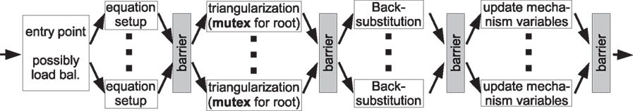
Figure 10. Flowchart illustrating how a time step is performed with multiple threads. While several barriers must be used to separate conflicting parts of the program, mutexes are used during triangularization when two threads access the same root compartment of a split cell.
Comparison to Existing Approaches
Previous attempts for parallel neural simulations were, to the authors’ best knowledge, mostly based on the message-passing paradigm (Bower and Beeman, 1998
; Hines et al., 2008a
,b
; Migliore et al., 2006
). A notable exception is NEST (Gewaltig and Diesmann, 2007
); this neural simulation software supports multithreading. However, its main application area are large networks of simple neurons each modeled with one or few compartments of the Integrate&Fire or Hodgkin–Huxley type, only, instead of anatomically and electrophysiologically detailed models.
In contrast, this work is based on biophysically detailed simulations with multithreading. The former restriction to message-passing environments lead to the far-reaching decision to not treat parallelization of equation setup and solving as independent tasks for several reasons:
• The simplest way to enhance an existing non-parallel neural simulator for message-passing environments is to support inter-cell-communication, i.e. sending and receiving synaptic currents, via messages as well. Also, this delivers good load balance for larger models and/or smaller clusters.
• For higher numbers of processors and/or lower numbers of cells, the most straightforward way to enhance the implementation is to support some kind of cell splitting and only transfer a set of split-compartment specific values between Gaussian elimination and back-substitution (see Hines et al., 2008a
). Thus, both equation setup and solving for a specific compartment are performed on the same PU.
• One of the main limiting factors in message-passing environments is communication latency; therefore, keeping the number of messages at a minimal level like the above mentioned techniques is crucial.
Message-passing programming can be difficult when existing programs are enhanced that were not designed with message-passing in mind from the beginning on. For instance, allowing equation setup and solving for a specific compartment to take place on different PUs as employed by the techniques introduced in this paper is rather difficult in message-passing environments. There, parts of the equations must be transferred between setup PU and solving PU before solving, and parts of the solution vector again must be transferred from the solving PU to the PU that sets up the equation again for the next time step.
In addition to programming issues, such an approach is not guaranteed to deliver proper performance because of both communication latency and bandwidth; overhead for message-passing might very well ruin what is gained by a better load balance during the equation setup stage. However, this depends on various parameters such as the model size, the number of PUs, the performance of cell splitting and the interconnection technology. Such an approach has not been implemented or tested and is a topic of further research.
The choice made thus far to bind equation setup and solving for a compartment to a specific PU results in a major limitation. Because the distribution of compartments onto PUs is governed by the dependencies of Gaussian elimination and back-substitution, load balancing problems in the solver stage are very severe because they apply to the much more time intensive mechanism computation stage as well. Proper balance in the solver stage is therefore of much more interest in message-passing based implementations and lead to techniques like splitcell and the sophisticated but complex multisplit method (Hines et al., 2008b
). This reveals why decoupling equation setup and solving is such an important concept in this work.
Another advantage of multithreaded programming can be observed when recalling the dynamic load balancing technique. It would be very hard to implement such a technique in a message-passing environment because not only would cells or parts of cells have to be loaded/unloaded during the simulation, but also would it be necessary to transmit data such as ion channel states or ion concentrations from the originally responsible process to the one taking over computation of these mechanism instances. In a multithreaded environment, however, dynamic load balancing reduces to simply changing thread specific start and stop indices of a loop over compartments.
There are more advantages to using a shared memory system. The simplicity of programming these systems, e.g. by using OpenMP to enhance existing C/C++/Fortran source code, combined with the intentional simplicity of the algorithms presented in here, makes these concepts applicable to custom simulation software. This is supported by the fact that virtually every modern operating system supports multithreading, while message-passing requires the installation of additional libraries and a comparatively complex run-time environment (regardless of the necessity to accommodate and administrate a computer cluster).
The most important novelty is the support for small models, however. The efficiency of simulating models in a parallel way directly depends on model size and inter-process communication latency. In general, computer clusters can only be used for rather large models with thousands or tens of thousands of compartments, not a very common case in every-day neural modeling. The main reason is that communication overhead for synchronization and data exchange quickly becomes the limiting factor when model size decreases. Multi-cores are fundamentally different in that inter-core communication only becomes a limiting factor once the model is so small that parallel simulation is not going to be of much use, anyway, because simulation times are short enough in the first place.
All measurements were performed on two systems running Ubuntu Linux 7.04, one equipped with two Xeon X5355 quad-cores, the other one with two Opteron K10 2347 quad-cores. They are illustrated in Figure 11
along with some benchmark results that are the topic of the next section.
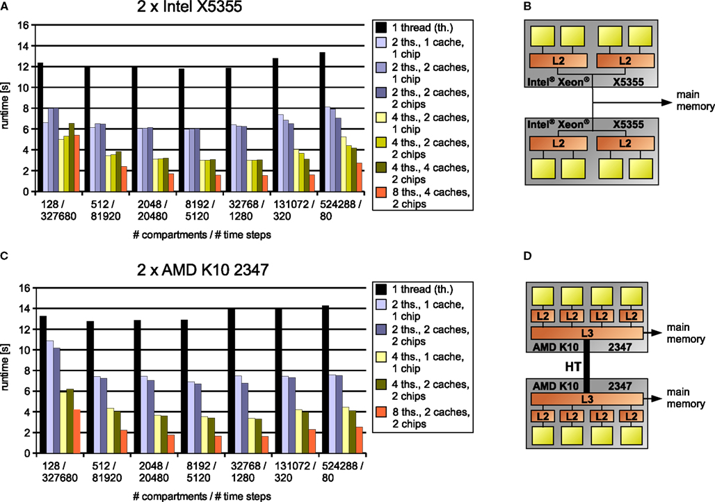
Figure 11. Results for simulations (A,C) on two test systems (B,D) of artificially generated models where computational complexity is held constant by varying both model size and number of time steps simultaneously, thus emphasizing the influence of inter-core communication and memory bandwidth. Legend right to the diagrams indicates number of threads, cache organization (number of L2 caches for Intel processor/number of L3 caches for the AMD processor) and whether the cores used are located on one or two chips. The connection between two chips on the AMD system (D) is illustrated by a thick line modeling the HyperTransport interconnect (HyperTransport Consortium, 2007
).
Influence of Cache Architecture and Model Complexity
The performance of algorithms and their implementations depends on many variables of both the input problem (the model) and the underlying architecture. To evaluate the influence of these parameters, we generated artificial models, each consisting of eight equally large neurons, each in turn modeled as eight connected cables, with a Hodgkin–Huxley mechanism on every compartment and one current injection mechanism per cell. This prevents cell splitting to influence the runtime. Between models, we varied the number of compartments and the number of simulated time steps while keeping the product of these two terms (and, thus, the computational work) at a constant value of 5 × 223. This allows us to emphasize the relative influence of architectural characteristics such as cache size and interconnection latency.
Panels A and C in Figure 11
depict the results obtained on our two test architectures; their structure, i.e. cores, caches and memory connection, are shown right to the results in Panels B and D. The model size, and thus the memory requirements, increase from left to right; the specific values for the number of compartments and the number of time steps are shown on the abscissa. For every model size, a number of bars are illustrated, each indicating the simulation runtime for a specific number of threads and what cores these threads were assigned to (i.e. cores with shared or separate caches, cores on the same or different chips etc.). Our aim is to show how runtime decreases with the number of threads and how this decrease depends on model size, cache size, cache architecture and memory requirements.
For the small 128-compartment model, the influence of inter-core communication for synchronizations is rather strong. Detailed benchmarks (not shown) indicate that when using two cores with separate caches on the Intel system, the two threads spend a total of about 20% of the overall runtime on waiting for other threads; on the AMD system, the cumulative synchronization time for two threads can be up to 40%. The reason for this big influence of synchronizations on the runtime is that their amount is proportional to the number of time steps and the number of cores. Accordingly, the cumulative time spent on synchronizations for the model with 512 compartments is approximately halved, thus having a much lower influence on the runtime. Even for 128 compartments, however, using two cores that share a cache on the Intel system gives a nearly linear speedup because of the low inter-core latency (the cumulative synchronization time is only 10% of the overall runtime).
We did not observe a similar effect on the AMD system; instead, we were surprised to see that using two cores with a shared L3 cache even leads to a lower runtime than using two cores with separate L3 caches on different chips, although in theory, communication should be slightly slower in the latter case. On the other hand, the AMD system exhibits better scaling for higher numbers of cores, even allowing for a speedup of 3.2; this means simulating 1 s of the 128 Hodgkin–Huxley compartments at a reasonable time step of 0.025 ms takes only about half a second.
For a wide range of model sizes, that is, from above 512 up to about 65.536 compartments (data for the latter not shown), we observe nearly linear and sometimes even superlinear speedups for two, four and eight threads. For this region of model sizes, the data fits largely into the cache(s) of the processor(s). The effect of the limited cache capacity can be seen clearly in the single-threaded case, where performance results are nearly constant up to a specific model size [16.384 (not shown) for the AMD, 32.768 for the Intel processor], reflecting the constant overall complexity. However, for larger models, the memory requirements significantly exceed the capacity of the core’s cache as estimated from the memory requirements per compartment (below 100 bytes). Thus, more data must be fetched from main memory, leading to a lower performance of the program. The same effect can be observed for two or more cores on the Intel system, depending on the cumulative cache size available to these cores – if two cores with their own caches are used, the cache size is effectively doubled, leading to a slightly better performance for these core combinations. This can be observed in Figure 11
for 131.072 compartments simulated on the Intel system; the effect is much less visible on the AMD system.
Another interesting observation is that on the Intel system, the bandwidth of the internal on-chip bus may be a limiting factor for large models. For the two largest models shown with 131.072 and 524.288 compartments, using combinations of two or four cores that lie on two chips gives better results than using the same number of cores located on one chip only, even if the cache size is the same.
The above results must be interpreted with the fact in mind that to rule out the effect of cell splitting, we used eight cells, thus avoiding the otherwise involved synchronization overhead. Also, the Hodgkin–Huxley mechanism was distributed homogeneously across the cell. In the next two sections, we will look at the influence of more heterogeneous mechanism placement and how iterative cell splitting helps for models with fewer cells.
Mechanism Computation
The measurements in Figure 11
did not take into account cell splitting nor multiple mechanisms and their heterogeneous distribution across a cell. Using artificial models again to test how well our sample implementation handles these challenges was not an option because the distribution of mechanism type complexities and mechanism instances is highly model specific.
Instead, we use a previously published hippocampal CA1 pyramidal cell model consisting of 600 compartments that was used in Migliore et al. (1999)
. In this work, distal dendritic compartments with a diameter lower than 0.5 μm or a distance larger than 500 μm from the soma were modeled with passive ion channels (and one with synapses), only. Other compartments, in contrast, are modeled using up to four different voltage-dependent ion channels, passive channels and current injections. Thereby, the overall mechanism complexity is distributed across the cell in a non-uniform manner, allowing to evaluate the performance of the dynamic load balancing technique introduced before. The automatic cell splitting algorithm split the CA1 model into two equally large pieces. In the single-threaded experiments, about 95% of the runtime were spent on mechanism setup.
Figure 12
shows the results for the two test systems and different numbers of threads. In the case of the rather small CA1 model, combinations of cores with rather low inter-core latency either yield slightly better (Intel X5355) or similar (AMD K10 2347) results; to keep Figure 12
simple, we only show the results obtained on the apparently best combination of cores for a fixed number of threads.
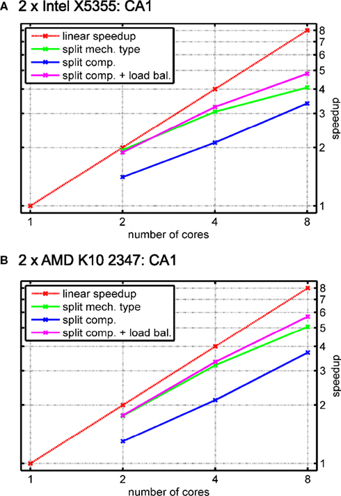
Figure 12. Simulation of a CA1 pyramidal cell with 600 compartments for 900 ms with a time step length of Δt = 0. 025 ms (see Migliore et al., 1999
). The cell is split into two equally large pieces; distal dendritic compartments do not use active channels, thus giving a heterogeneous mechanism distribution across the cell. (A) Speedup results on the Intel test system (see Figure 11
A). Red line: linear speedup; green: measured speedups of mechanism type level parallelization (Figure 5
); blue: compartment level parallelization (Figure 7
) without load-balancing for taking into account heterogeneous mechanism distribution across cell; magenta: compartment level parallelization with load-balancing. (B) Same as (A) on the AMD test system (Figure 11
C).
The figure shows a red line for the linear speedup along with speedups obtained with two, four and eight cores. Three kinds of mechanism computation strategies are illustrated; splitting up the list of instances for each mechanism type (green) and splitting up the number of compartments into equally large sets without (blue) and with subsequent load balancing (magenta). Due to the increase in synchronization overhead, splitting up mechanism types is either as good as or worse than splitting up compartments with load balancing. Another advantage of the compartment level parallelization method is less transmission of equations between cores as an equation is set up by one core, only. In contrast, for mechanism type level parallelization, different cores may actually compute mechanisms for the same compartment if mechanism placement is heterogeneous, leading to additional inter-core communication. The third method, splitting up compartments into equally large sets without load balancing, is depicted to illustrate the need for dynamically resizing the sets of compartments due to the heterogeneity in mechanism placement.
The general observation regarding dynamic load balancing is that virtually no overhead is induced by both measuring mechanism type complexities and resizing the sets of compartments. It is remarkable that the implementation gives proper speedups even for such small models when using the original model’s simulation time length of 90 ms – a runtime reduction from 1.55 s (1.81 s) to about 0.31 s (0.33 s) for eight cores is not only sufficient for most users that perform simulations in an interactive manner but also facilitates automatic optimizations that require several subsequent single simulation runs with adapted parameters.
Automatic Cell Splitting and Distribution
The remaining question is how well the cell splitting algorithm works. Again, it was not possible to use artificially generated models; the distribution of cell sizes and cell geometry is highly variable, and the number of compartments used for modeling a cell is user-defined. For instance, the above mentioned CA1 cell could be split into two equally large pieces, while other cells result in three or more subtrees of different sizes.
To give an intuition of how the algorithm works, we will use a sample model of the blowfly’s HS network, published in Borst and Haag (1996)
. The three cells (HSE, HSS and HSN) were reconstructed from cobalt-filled cells; they are comprised of 11497, 10824 and 9004 compartments, respectively. Every compartment was modeled with a mechanism for passive ion channels, only, and one current injection per cell; in the single-threaded experiments, about 43% of the runtime were spent on mechanism setup. Again, only the results for combinations of cores that gave the best results are shown.
Figure 13
shows performance results for the HS network and different numbers of cores for the cases when either (automatic) cell splitting is disabled (green line) or enabled (red line). In the case of two cells, the splitting algorithm stops after splitting only the largest of the three cells because a distribution of 15628 vs. 15696 compartments per core is achieved; in contrast, not using cell splitting gives a rather poor balance of 19828 vs. 11497 compartments, i.e. an imbalance of 29.8% of the overall number of compartments.
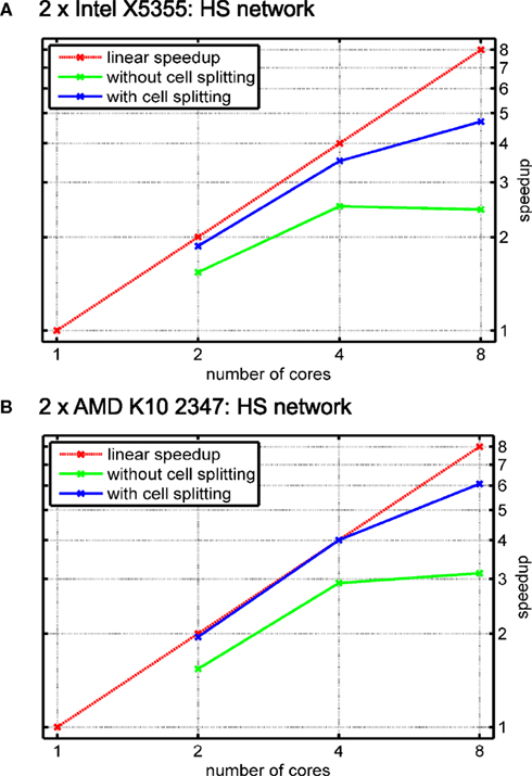
Figure 13. Simulation of the blowfly’s HS network with automatic cell splitting disabled and enabled. The model was simulated for 100 ms with a time step length of Δt = 0.025 ms. (A) Speedup results on the Intel test system (see Figure 11
A). Green line shows speedup measurements when the three cells were solved without splitting them; blue line shows results with cell splitting. The relative influence of cell splitting increases with increasing numbers of cores. (B) Same as (A) on the AMD test system.
The relative effect on runtime is even more significant for four cores when automatic cell splitting reduces imbalance from now 36.7% to 4.4%; on eight cores, the imbalance is reduced from 36.7% to 9.9%.
Figure 13
reflects the importance of cell splitting, especially for higher numbers of cores. The reason why the effect of cell splitting plays such a big role for the HS model is that it uses the computationally cheap mechanism for passive ion channels, only. Thus, the effect of the solver stage is much bigger than for models with more complex ion channel mechanisms. An additional effect of either not splitting cells at all, or having to few subtrees to assign to cores, is that an equation must be transferred from the core that sets it up and the core that solves it, and vice-versa once the resulting voltage has been computed. If these cores share a cache, or if the time spent on equation setup is large enough, this effect is very small, but it can play a role for computationally simple models or in cases where there are many more cores than cells/subtrees. Thus, the influence of cell splitting strongly depends on the number of cores. In general, when the number of cells is higher than the number of cores, whole-cell balancing is often sufficient. Also, a high mechanism complexity may strongly reduce the portion of time spent in solving the equations and therefore the influence of cell splitting.
In this paper, we presented algorithms and an implementation thereof for the parallel execution of biophysically realistic neural simulations using multithreading. To our knowledge, this is the first manuscript solely based on multithreading; our focus lies on both advantages and caveats of multi-core architectures. Our sample implementation is a lightweight simulator based on the numerical core of NEURON; it is freely available for studying, testing and extending the code. Our algorithms often scale linearly and sometimes superlinearly with the number of cores over a wide range of the common complexities of neuronal models.
Scalability is limited mainly in three cases. First, for smaller models (up to approximately 256 compartments), synchronizations between cores comprise a relatively large portion of a time step. The strength of this effect depends on the cache-architecture and the number of cores used. This observation is not specific to our algorithms or neural simulations but a general problem in parallel programming; rather, we would like to point out that even for such small models, multi-cores are able to decrease execution times significantly.
Second, once models do not fit into the cache any more, decreases in performance can be observed for both the single-threaded and the multi-threaded code, and speedups become sublinear to an extent depending on the number of threads and the architecture. In our measurements, this effect sets in at about 33.000/66.000 (AMD/Intel) Hodgkin–Huxley compartments for a single thread, depending on the cache-size used. For eight threads, this effect only sets in at 131.000/262.000 Hodgkin–Huxley compartments, an unusually big model size.
Third, our cell splitting and balancing algorithm may lead to increased inter-core communication if the number of cores is significantly higher than the number of cells. The strength of this effect depends on the number of cells, the cache-architecture and the ratio of time spent on solving.
It is not easy to predict how well the concepts will work on future multi-cores comprised of 32 or more chips, because inter-core latency already is an issue, and memory bandwidth is likely to become a limiting factor for bigger models if all cores use a common front side bus. One possible development is the shift towards NUMA (Non-Uniform Memory Architecture) multicore architectures where different memory controllers instead of one central memory controller are used. These architectures, already employed in multi-core systems with AMD processors, have the potential to solve the scalability issue; however, we observed rather high inter-core communication latencies on our AMD test system even for cores that have a common L3 cache.
The authors declare that the research was conducted in the absence of any commercial or financial relationships that could be construed as a potential conflict of interest.
This work was supported by the Max-Planck-Society. The authors would like to thank Michael Hines for fruitful discussions and comments on the paper and the LRR department at Technical University of Munich for providing us with the necessary computer systems.
- ^ This is not necessarily the case for programs that are interpreted by another program such as MATLAB or IDL code; here, the intermediate software layer may automatically identify workload distributions for simple operations such as matrix multiplications and execute them in parallel transparently for the original program (ITT Visual Information Solutions, 2007 ; Moler, 2007 ).
- ^ The only exceptions are the stack and Thread Local Storage.
- ^ Electrical synapses/gap junctions can be modeled in a manner similar to the axial terms; however, this prohibits the usage of a highly optimized Gaussian elimination method presented in the next section. Therefore, we assume gap junctions to be modeled as mechanisms with the respective approximation.
- ^ Examining our and NEURON’s assembler code produced by the compiler for the passive mechanism leads us to the hypothesis that a different order of floating point operations generated for effectively the same computations is responsible for these deviations.
- ^ Mechanism currents at the next time step are estimated based on known values from the current time step. This approximation, which is specific to implicit methods, is explained in Sections 4.3 and Appendix A in Eichner (2007) and pp. 168–169 in Carnevale and Hines (2006) .
- ^ Representing connections between cells with off-diagonal elements works only for currents linear in the voltage difference, i.e. Iij = g(Vj − Vi). This holds true for axial resistances and could be used for gap junctions as well but does not work for chemical synapses. Modeling gap junctions with off-diagonal entries prohibits the usage of the efficient solver algorithm presented in the section “Compartmental Modeling”, however, while not increasing accuracy significantly.
AMD, Inc. (2007b). AMD Opteron Processor Family. Available at: http://www.amd.com/opteron
.
Drepper, U., and Molnar, I. (2005). The Native POSIX Thread Library for Linux. Available at: http://people.redhat.com/drepper/nptl-design pdf
.
Eichner, H. (2007). Biophysically Realistic Simulations on Multi-Core Architectures. Available at: http://www.neuro.mpg.de/english/rd/scn/research/ModelFly_Project/downloads/Eichner_thesis.pdf
.
Intel Corp. (2006). Intel Core Microarchitecture. Available at: http://www.intel.com/technology/architecture-silicon/core/
.
ITT Visual Information Solutions (2007). Multi-Threading in IDL. Available at: http://www.ittvis.com/idl/pdfs/IDL_MultiThread.pdf
.
Korf, R. E. (1997). A Complete Anytime Algorithm for Number Partitioning. Available at: http://web.cecs.pdx.edu/bart/cs510cs/papers/korf-ckk.pdf
, section 2.5.