1
Washington University, Department of Biomedical Engineering, St Louis, MO, USA
2
Kyoto University, Human Brain Research Center, Kyoto, Japan
3
Washington University School of Medicine, St Louis, USA
4
Kyoto Prefectural University of Medicine, Department of Physiology, Kyoto, Japan
We used in vivo voltage-sensitive dye optical imaging to examine the cortical representation of interaural time difference (ITD), which is believed to be involved in sound source localization. We found that acoustic stimuli with dissimilar ITD activate various localized domains in the auditory cortex. The main loci of the activation pattern shift up to 1 mm during the first 40 ms of the response period. We suppose that some of the neurons in each pool are sensitive to the definite ITD and involved in the transduction of information about sound source localization, based on the ITD. This assumption gives a reasonable fit to the Jeffress model in which the neural network calculates the ITD to define the direction of the sound source. Such calculation forms the basis for the cortex’s ability to detect the azimuth of the sound source.
As is well known, one of the main structural principles of the auditory cortex is tonotopicity (Ehret, 1997
). In the auditory cortex of higher mammals, isofrequency areas appear in the form of elongated spots orthogonal to the rostro-caudal axis (Eggermont, 2006
; Ehret, 1997
; Sally and Kelly, 1988
). In a predator’s AI (primary auditory cortex), high-frequency representations are located in the rostral area and low-frequency representations in the caudal area. Primates demonstrate similar structure; low frequencies are represented anterolaterally, high frequencies posteromedially in AI. (Furukawa and Middlebrooks, 2002
; Hosokawa et al., 2004
; Tokioka et al., 2000
).
Voltage-sensitive dyes (VSD) fluoresce proportional to changes in transmembrane potential, and thus can be used to detect neural activity (Grinvald et al., 2001
). Using modern charge couple devices (CCD – cameras), functional mapping of the neocortex can achieve a very high spatial resolution (Grinvald et al., 2001
; Inyushin et al., 2001
). VSD imaging has been proven as a powerful tool for the investigation of the functional architecture of the auditory cortex (Grinvald et al., 2001
; Nishimura et al., 2006
; Song et al., 2006
) and cochlear nucleus (Kaltenbach and Zhang, 2004
).
In vivo VSD optical imaging allows us to make functional maps of the neocortex, and, in the case of imaging the auditory cortex, satisfy the question of where the neural pools responsible for sound source localization are located in the brain (Eggermont, 2006
; Jenkins and Merzenich, 1984
; Spitzer and Takahashi, 2006
; Tsytsarev and Tanaka, 2002
). In other words, the critical problem in neural network studies is how the computational ability of the neural network in the neocortex can be applied to define the location of sound sources.
Animals can usually localize sound clicks in the horizontal dimension. However, when two clicks presented to the left and right ears are separated by a short time delay, the animal can experience an illusion, failing to properly localize the sound (Figure 1
). In the present study, we demonstrate that the spatial distribution of sound sources is not only reflected by cortical activity but also creates patterns similar to a set of moving activated spots, each representing a specific azimuth angle toward the object.
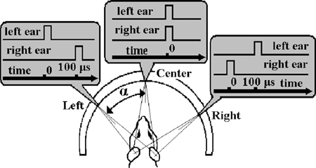
Figure 1. Binaural click produces the sensation of a sound source to the left, straight ahead, or to the right of the animal. The angle is determined by the Interaural Time Difference (ITD). It is important to note that the relationship between angle and duration of ITD is approximate since the shape, orientation, and movement of the animal’s head has an influence to some extent as well as the harmonics of the sound counter. Time scales and zero-markings are for each of the three different ITDs.
Imaging was performed in 12 adult rats (Sprague–Dawley, weight 250–300 g, age 2–3 months) that were anesthetized with a mixture of ketamine (90 mg/kg, i.p. Ketalar-50, Parke-Davis) and xylazine (12 mg/kg, i.p., Bayer Corp). Supplementary ketamine hydrochloride (40 mg/kg body weight, i.m.) was injected about 1 h later to maintain a constant level of anesthesia during the experiment (Tsytsarev and Tanaka, 2002
). The anesthesia level was determined based on the heart rate, which was continuously monitored using an electrocardiomonitor. At the end of each experiment, the animal was sacrificed using an overdose of Nembutal (200 mg/kg body weight, i.p., Bayer Corp.). All procedures were carried out according to the standards of the Animal Care Committee of Kyoto Prefecture University of Medicine.
A detailed description of the experimental technique can be found in cited references Bonhoeffer and Grinvald (1996) and Grinvald et al. (2001)
. The animal was fixed on the stereotaxic frame using ear bars with channels that allowed sound transduction into the middle ear (Tsytsarev et al., 2004
). The skin and muscles of the dorsolateral part of the head were surgically excised and the left lateral wall of the skull was exposed from the muscles. The cranium above the auditory cortex was removed using a dental drill, and a recording chamber made of dental wax (4–6 mm i.d., height 2–3 mm) was constructed above the hole in the skull (Bahar et al., 2006
; Ojima et al., 2005
). The dura mater over the auditory cortex was removed and the brain was covered with artificial cerebrospinal fluid (ACSF) at a temperature of 30–35°C (Mrsic-Flogel et al., 2005
; Takashima et al., 2005
; Versnel et al., 2002
). The VSD RH-795 (Molecular Probes, 0.6 mg/ml in ACSF), was applied to the exposed cortex for approximately 45 min. After staining, the cortex was washed with dye-free ACSF for approximately 15 min (Grinvald et al., 2001
). A CCD camera (MiCAM-01, Brain Vision Inc., 2002, Japan, http://www.scimedia.com
), (90 × 60 pixels, 0.7 ms/frame) then positioned above the chamber and directed such that its optical axis was perpendicular to the cortical surface.
The focusing plane was manipulated 400 μm below the cortical surface. The recording area of the cortex was illuminated with a 540 nm wavelength light via a cube-system with two optic filters and a dichroic mirror. At the start of each optical recording, a gray-scale image of the region of interest was obtained. Each stimulus consisted of a pair of 30 μs square-pulse binaural clicks with interaural time difference (ITD) 0 or 100 μs (Figure 1
). During recording, stimuli with different ITDs were presented in a quasi-random sequence starting at the tenth frame with a 4 s interval in between. Since heart rhythm produces sudden changes in fluorescence during a heart contraction, a light path shutter was synchronized with the electrocardiogram: the light shutter was opened only during the period between two consecutive heartbeats in order to minimize light exposure and prevent dye bleaching. We used a University constructed low-noise shutter and a special technique from our previous studies (Tsytsarev and Tanaka, 2002
; Tsytsarev et al., 2006
) for minimization of shutter noise. In short, after insertion of the earphones into the ears the auricles were filled with Vaseline and the ears were wrapped with tape. To prevent a sound advancing through the metal apparatus, a stereotaxic frame was placed on the foam-rubber plate. As was shown in previous electrophysiological studies, (Tsytsarev et al., 2006
) such an experimental set up prevents the shutter sound from confounding the results. To set an electrocardiogram threshold the shutter was controlled by a differential alternating current amplifier (model 1700, AM Systems Inc, WA, USA) with window discriminator (WD01, Scientific Ltd, UK). Thus, the sequence of the stimulation and recording of evoked optical signal was as follows: Heart beat, shutter opening, start of the optical signal recording, 10 ms pause, sound stimulation, end of recording trial (after a total recording time of 82 ms), shutter closing.
Four pilot experiments with pure tone binaural stimulation and wideband sound clicks were performed to test our method. The sound stimuli had frequencies of 1, 5, and 7 kHz and a duration of 40 ms. The linearly increasing onset and decreasing offset of stimulus envelopes were set at 5 ms. All stimuli were calibrated before optical recording and the sound pressure was set at 45 dB. As in the previously described method, (Nishimura et al., 2007
; Tsytsarev and Tanaka, 2002
) the images were combined to construct a frequency map (Figure 2
A). As expected, the tonotopic representation of sound frequencies in these experiments demonstrated that the location and direction of sound frequency arrangement closely agrees with previously obtained data (Kalatsky et al., 2005
; Nishimura et al., 2007
; Takahashi et al., 2004
; Tsytsarev et al., 2006
). On that ground, we concluded that our method was sufficiently reliable and proceeded to test the sound stimuli with various ITD.
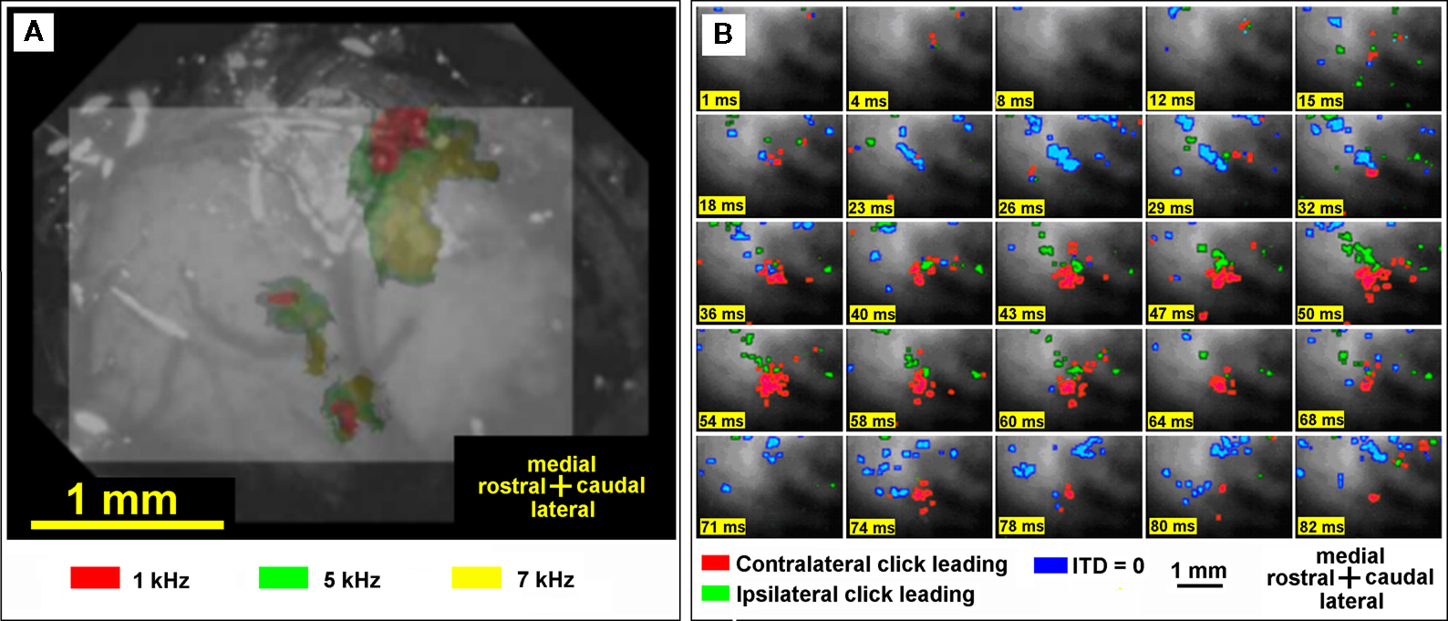
Figure 2. (A) Color-coded tonotopic map of sound frequencies showing the organization of subfields of the auditory cortex. Cortical domains significantly activated by presentation of three sound frequencies are indicated by different colors, as indicated in the key on the bottom of the figure. (B) Optical evoked activity maps with three different stimuli with interaural time difference (ITD) 100 ms. Click leading: red – contralateral, green – ipsilateral, blue – both clicks are presented simultaneously (ITD = 0). Number of trials 20, sound stimulus onset at 10 ms.
Analysis of the recorded image data was performed using Brain Vision Analyzer (©, Brain Vision Inc., Tokyo, Japan). Presentation of sound stimuli took place after the first 10 frames so data prior to frame 10 contains only random non-sound-evoked fluctuations. To extract the images reflecting neural activity in response to sound stimuli, we applied “first-frame analysis,” in which signals in the first 10 prestimulus frames (averaged from multiple trials) were subtracted from signals in the subsequent frames (Bonhoeffer and Grinvald, 1996
). In the simplest case of “first-frame analysis” the first prestimulus frame must be subtracted from each subsequent frame, but we used an averaged value of 10 prestimulus frames instead (Tsytsarev et al., 2004
). This procedure was applied to the recorded signals at each trial, which were then averaged. We then reconstructed optical signals elicited in response to each acoustic stimulus using the generalized indicator function method, which projects the optical imaging data onto a subspace of high signal-to-noise ratio (Bonhoeffer and Grinvald, 1996
).
The temporal changes of the fluorescence after the stimulus onset were examined in a small rectangular domain of 2 × 2 pixels. This domain was chosen in order to avoid intersecting any blood vessels. To eliminate fluctuation of the signal strength between individual rats we normalized the signals using the maximum ΔF/F in response to contralateral stimulation before the intertrial averaging procedure. The temporal changes of the optical signal are shown in Figure 2
B. To construct color-coded maps and determine the areas significantly activated by a particular ITD, the images of optical signals were thresholded by 50% of the maximum response inside the area of recording. Thus, we obtained maps of strongly activated areas that were color-coded according to the ITD of the stimuli.
Optical signals evoked by a binaural click stimulus at a sound pressure level of 45 dB were recorded in each rat. Figure 3
displays the time courses of optical images in rat auditory cortex as a result of optical evoked activity produced with three different stimuli: ipsi- and contralateral click leading with ITD of 100 μs, and simultaneous click in both ears. Figure 3
shows three separate experiments with three different rats tracing the dynamic patterns of the evoked activity. As expected, each stimulus induced activity in several small cortex areas. These areas do not have definite form and can change in just tens of milliseconds. Such patterns were observed in all experiments.
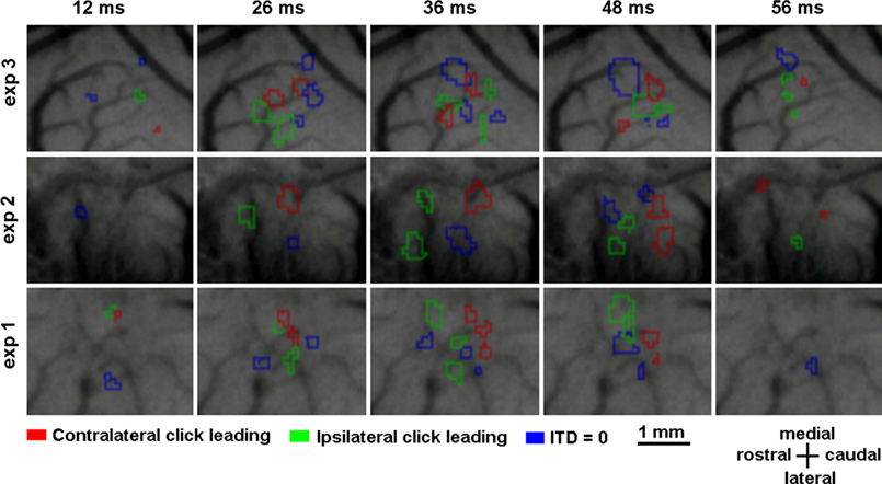
Figure 3. Optical evoked activity maps for three experiments with three different animals. Time after stimulus onset is specified at the top of each column. The data has been averaged over 20 trials.
Figure 4
shows the temporal evolution of the spatial pattern of optical signals evoked by one particular sound stimulus (ITD 100 μs, contralateral click leading). We can observe that the shape of the activated area changes over time following stimulus onset. For all stimuli, activated areas steadily increase from the 15th to 50th ms and then decrease; the activated domains appear as irregularly shaped spots.
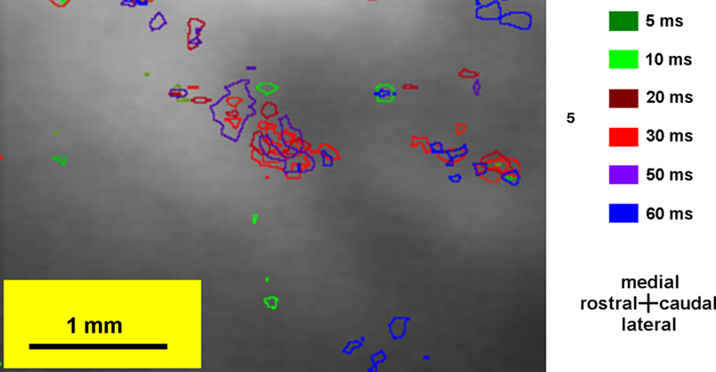
Figure 4. Optical evoked activity map. Interaural time difference is 100 ms, contralateral click leading. Color designates time delay from stimulus onset.
In all cases, we found that sound stimuli with different ITD led to different cortical activation patterns. But, in an experiment with a single animal, various sessions produced the same patterns with each separate ITD. One ITD typically activated two spatially disconnected regions (Figure 3
). The patterns were randomly distributed and had irregular shapes. The activated patterns moved around the cortex within 0.1–0.3 mm; there is no statistically significant difference between the movements of activations caused by different stimuli (P = 0.963). The mean velocity was 5.8 mm/s, which was found to be significantly differentially expressed [one way analysis of variance (ANOVA) P < 0.01]. The absolute displacement was close in all experiments with little statistical straggling. In all cases, the response reached its maximum value after 30–40 ms (Figures 5
A–C). At the same time, we did not find any systematic character in the latency period changes of each pattern with different ITD. The results obtained in different sessions (which took place one after another) with the same animal were practically identical. These results suggest that any complete explanation of the cortical representation of the ITD must incorporate the temporal characteristics of the neuronal response patterns.
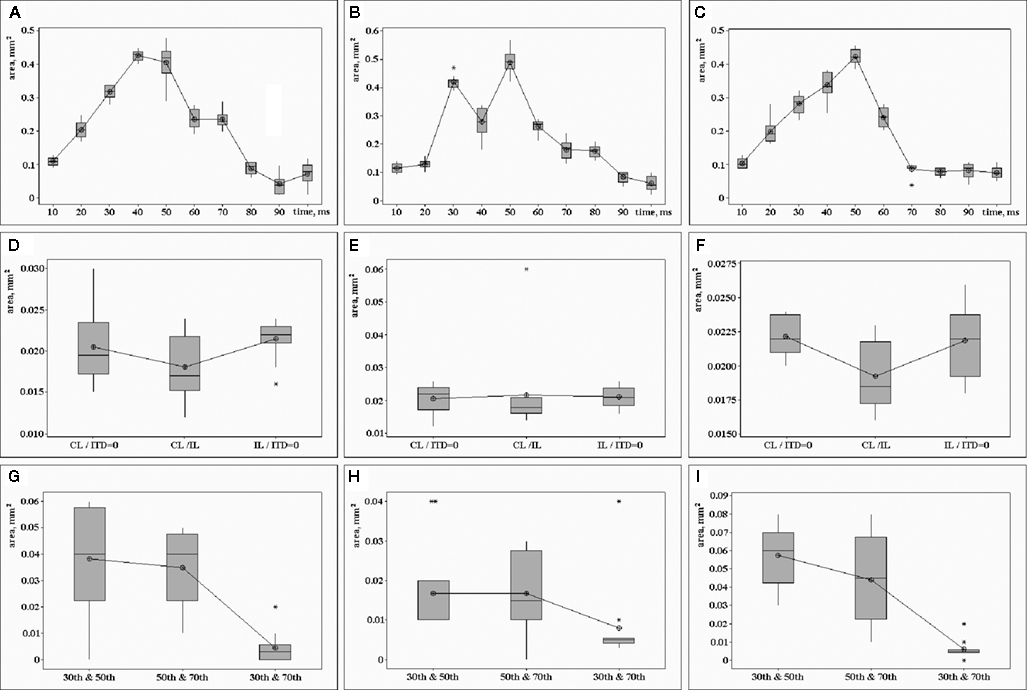
Figure 5. The area where the voltage-sensitive dye signal exceeds 50% of the maximum response within the area of recording. Top row: (A) contralateral click led (CL), (B) simultaneous contra- and ipsilateral clicks (ITD = 0), (C) ipsilateral click led (IL). Period of time from the sound stimulus onset (millisecond) is shown along the horizontal axis, size of the activated area (square millimeter) is shown along the vertical axis. Middle row: the size of the activated area subject to various pairs of clicks and the period of time after stimulus onset. Three types of pairs are shown along the horizontal axis: CL/ITD = 0 – contralateral click leaded (CL) and both clicks presented simultaneously (ITD = 0), CL/IL – contralateral click leaded (CL) and ipsilateral click leaded (L-100-R), IL/ITD = 0 – ipsilateral click leaded (IL) and both clicks presented simultaneously (ITD = 0). Three periods of time after stimuli onset: (D) 30 ms, (E) 50 ms, (F) 70 ms. The size of the superimposition of the cortical areas is shown along the vertical axis (square millimeter). Bottom row: the common area (size is shown along the vertical axis, mm) of the cortical parts, activated at the 30th and 50th, or 50th and 70th, or 30th and 70th ms after stimulus onset: (G) ipsilateral click led stimuli (IL), (H) both clicks presented simultaneously (ITD = 0), (I) contralateral click led stimuli (CL). Standard deviation for n = 12 is shown along the vertical axis in all frames.
We found that each ITD usually corresponded to a common pattern. From the time of origination until the disappearance of the pattern, its spatial extent approximately doubled and then decreased. At the maximum size, the patterns covered an area of 0.2–0.4 mm.
Comparative analysis of the areas activated by two different stimuli or by the same stimulus at different times after stimulus onset was completed. After setting the threshold at 50% (see Materials and Methods), the sizes of the superposed areas were calculated and averaged. Results of this analysis are presented in Figure 5
.
Figure 5
shows superimposition of the areas activated by different stimuli at the same time after a stimulus onset of 30 ms (Figure 5
D), 50 ms (Figure 5
E), and 70 ms (Figure 5
F). The sizes of the cortical parts activated by different stimuli are very similar (0.01–0.02 mm). They remain stable at the 30th, 50th, and 70th ms after stimulus onset. The common area of the cortical parts, activated at the 30th and 70th ms after stimulus onset is much smaller than areas activated at the 30th and 50th ms or the 50th and 70th ms (Figures 5
G–I). This regularity is significant for all stimuli, although the effect is smaller for stimuli with an ITD of 0 (ANOVA P < 0.01).
Topographical representation is a main feature of the sensory cortices of mammals. The primary somatosensory cortex contains a somatotopic map of the body, the primary visual cortex contains a retinotopic map of the visual field, and the primary auditory cortex (AI) contains a tonotopic map of sound frequency. Based on this principle, many scientists expect the presence of a spatial auditory map.
In 1950 this hypothesis was proposed by Jeffress and has been discussed by many authors during the last decade (King et al., 2001
; McAlpine and Grothe, 2003
; McAlpine et al., 2001
; Zador, 2001
). The features of the representation of auditory space in the brain have been observed in the superior colliculus (King et al., 2001
; Nelken et al., 2004
) for mammals and in the thalamus (Proctor and Konishi, 1997
) for avians. Nevertheless, spatial representation of sound source has not been demonstrated in the mammalian neocortex. It is hypothesized that ITD are calculated in the superior olivary nucleus of the brainstem (Tollin, 2003
), where neurons with various connecting axon lengths receive innervations from each ear.
Many authors (McAlpine and Grothe, 2003
; McAlpine et al., 2001
; Mrsic-Flogel et al., 2005
) suppose that if the Jeffress model is correct, the various cues of virtual auditory space might be integrated into a tonotopic map. Numerous scientists, however, have failed to find the auditory space map in the mammalian neocortex (Furukawa and Middlebrooks, 2002
; Mickey and Middlebrooks, 2005
). However, such a map being described in the owl’s thalamus has given hope to the prospect of finding one in mammals (Proctor and Konishi, 1997
). In spite of the fact that a representation of the sound source in the neocortex of mammals has not been found, work in recent decades has shown that separate neurons of the AI have the property of definite spatial selectivity (Doan and Saunders, 1999
; Furukawa and Middlebrooks, 2002
; Kelly and Phillips, 1991
; Mickey and Middlebrooks, 2005
; Mrsic-Flogel et al., 2005
).
Jeffress developed the first model for sound localization using a projective interference circuit (Mrsic-Flogel et al., 2005
; Nelken et al., 2004
), noise originating from an external source to the right which interferes with leftward excitation and visa versa. Malhotra et al. (2004)
used terms “what” and “where” to denote different processes of sound perception. It seems reasonable to say that the “what” and “where” processing in non-primary auditory cortex can be divided among the anterior and posterior auditory fields, as was demonstrated by Malhotra et al. (2004)
. It is therefore possible that the location of a sound source is inferentially represented by the tonotopically organized arrays of auditory neurons as a spatiotemporal population code.
Several lesion studies suggest that AI is required for sound source localization in carnivores (Kummierek et al., 2007
), primates, (Kummierek et al., 2007
) and martens (Smith et al., 2004
), but the question of how different fields of the rodent’s auditory cortex relate to each other in the sound localization process is still just beginning to be explored. Numerous studies using anesthetized animals have consistently found that many neurons of the auditory cortex are sensitive to sound source location, but topographical representation of space has not been demonstrated (Furukawa and Middlebrooks, 2002
; Kalatsky et al., 2005
; King et al., 2001
).
However, our experimental data implies that the ITD-receptive patterns originate from the interaction between the frequency and non-frequency sensitivity of cortical neurons. One could say the ITD-activated patterns shift in ways that are directly related to individual acoustic cue response differences between animals.
It has been reported that the auditory cortical neurons encode some sound parameters, such as duration, frequency preference, and ipsi-, contra-or bilateral preference (Barbour and Wang, 2002
; Ehret, 1997
). We suppose that some neurons might be organized into an ITD-preferred pool. In light of the present study, the cortical areas involved in spatial localization clearly contain more than one region of auditory cortex. It has been shown previously that the neuronal spike patterns in the auditory cortex represent information about the azimuth of the sound source (Furukawa and Middlebrooks, 2002
; Mickey and Middlebrooks, 2005
) and that these neurons are distributed widely throughout the auditory cortex.
Our results demonstrate that patterns of neural activity recorded in response to binaural click presentations can encode ITD. Based upon the data presented here, we conclude that some neurons in the auditory cortex receive information from several neural pools, each of which processes separate stimuli. The ITD information is then converted into neural code and passed to the auditory cortex.
A standout feature of these domains is their tendency to shift in space over time. Even though these movements can become relatively large, the regions never overlap by more than approximately 25% of their total size. Additionally, no two regions ever occupy the exact same spot, even at different time points. These facts help show that the areas remain spatially segregated despite their tendency to move.
In 2001, we showed that acoustic stimuli with distinct ITD activated various domains localized in AI (Tsytsarev and Tanaka, 2002
). It is important to note that the center of the activated domain shifted as the time difference was changed (Tsytsarev and Tanaka, 2002
). In our opinion, this fact, taken together with the idea that ITD plays an important role in sound source localization, suggests that AI is involved in information transformation from ITD to sound source location. Obtained results show that the cortical representation of sound sources is reflected by neural activity and creates a pattern like a “moving (floating?) mosaic”. The data presented here enable us – despite the fact that the virtual map of auditory space in rat auditory cortex does not exist – to suppose that the neurons which are selectively sensitive to different ITDs are structured in definite groups. Overall, the present study demonstrates the effectiveness of the neuronal ensemble coding of a range of different ITDs. Further studies will be necessary to identify details of information-bearing features and the neural mechanisms of ITD and its transduction into source localization. Further investigation with more modern VSD and CCD cameras may help discover more about how the spatial-temporal patterns of the auditory cortex convey information that can be related to sound source localization.
The authors declare that the research was conducted in the absence of any commercial or financial relationships that could be construed as a potential conflict of interest.
We want to express our undying gratitude to Dr. Sonya Bahar for her great help in preparing and editing the manuscript. We also thank Dr. Shuji Higashi and Dr. Hitoshi Inokawa (Division of Neurophysiology, Kyoto Prefecture University of Medicine) for valuable advice and technical support in all our experiments, Dr. Zador, Dr. Liberman and Dr. Hiken for their advice in writing the manuscript and Dr. Astafiev for his help in labor management.
Grinvald, A., Shoham, D., Shmuel, A., Glaser, D., Vanzetta, I., Shtoyerman, E., Slovin, H., Sterkin, A., Wijnbergen, C., Hildesheim, R., and Arieli, A. (2001). In Vivo Optical Imaging of Cortical Architecture and Dynamics. The Grodetsky Center for Research of Higher Brain Functions, the Weizman Institute of Science. Technical Report GC-AG/99-6.
Song, W. J., Kawaguchi, H., Totoki, S., Inoue, Y., Katura, T., Maeda, S., Inagaki, S., Shirasawa, H., and Nishimura, M. (2006). Cortical intrinsic circuits can support activity propagation through an isofrequency strip of the guinea pig primary auditory cortex. Cereb. Cortex 16, 718–729. doi:10.1093/cercor/bhj018.