Tied Free-Field boundaries to enhance numerical accuracy of earthquake simulations

Free-Field (FF) boundaries have previously been developed to replicate the (infinite) far-free-field domain in the simulation of earthquake loading problems. Although they can yield accurate results under certain conditions, it has been observed that significant problems can occur if the behaviour of the material near the boundaries is highly non-linear or incorporates cyclic attributes, or if the boundaries are located close to the domain of interest. To address the inaccuracies caused by the use of traditional FF boundaries, a novel technique is proposed: Tied Free-Fields. This technique combines the principles of both standard earthquake boundary conditions (that is, Tied-Degree (TD) and FF boundaries) to accommodate earthquake loading at the domain boundaries in a direct and economical fashion. The proposed solution has been tested using one and two-dimensional benchmarks and an advanced constitutive model. The results show a significant improvement in accuracy over traditional FF boundaries in the modelling of surface settlements and computed energy released, as well as a significant improvement in computational efficiency over TD boundaries in the modelling of asymmetric problem domains.

1 Introduction

In geotechnical engineering, earthquakes present significant hazards due to their destructive nature (Budimir et al., 2014). Hence, seismic numerical research has grown rapidly, encompassing areas such as liquefaction triggering (Ye and Wang, 2016; González Acosta et al., 2022), post-earthquake settlements (Ziotopoulou and Boulanger, 2013; Basu et al., 2022), and soil–structure interaction (Torabi and Rayhani, 2014; Luque and Bray, 2020). Nonetheless, in the analysis of dynamic problems, the implementation and use of appropriate boundary conditions are imperative to guarantee the realistic simulation and resolution of a problem. Several methods have been developed to address the problem of absorbing spurious dynamic waves at the domain boundary, demonstrating significant benefits for the analysis of dynamic geotechnical problems (Chapel, 1987; Davoodi et al., 2018; Do et al., 2022). In this field, the most well-known boundaries include the standard viscous boundary (Lysmer and Kuhlemeyer, 1969), the cone boundary (Kellezi, 1998), the superposition boundary (Smith, 1974), the boundary element method (Mansur, 1983), the perfectly matched layer (Basu and Chopra, 2003), and the infinite elements method (Bettess, 1977). Other less prevalent methods include, for example, paraxial boundaries (Clayton and Engquist, 1977; Modaressi and Benzenati, 1992; Xu et al., 2017), the incremental damping method (Semblat et al., 2010), and high-order absorbing boundaries (Hagstrom and Warburton, 2004). A comprehensive list of diverse absorbing boundaries implemented in numerical analysis can be found in Kontoe (2006), Hu et al. (2020), and Li et al. (2018).

However, despite the substantial number of boundaries developed to absorb radiation waves (i.e., excitations originating within the model and extending to the boundaries), few boundaries have been designed to simulate earthquake conditions (i.e., to replicate the infinite free-field response that induces inward lateral excitations as nodal dynamic loads). To date, some of the best-performing boundaries for handling earthquake-transmitted loading inwards are Tied-Degree (TD) and Free-Field (FF) boundaries [both elaborated in Zienkiewicz et al. (1989)], and the Domain Reduction Method (DRM) (Bielak et al., 2003), all of which have been implemented and compared in multiple studies (e.g., Li et al., 2018; Galavi et al., 2013; Kontoe et al., 2009; Bielak and Loukakis, 2025).

Among these three types of boundaries, Free-Field (FF) boundaries are generally the most advantageous, due to their easy implementation in combination with their ability to be integrated with a two-dimensional (2D) domain, even when the lateral boundaries are non-symmetric. However, when FF boundaries are employed, it is necessary to incorporate simpler linear or nonlinear elasto-plastic materials, such as Mohr–Coulomb and Hardening Soil Small (Benz, 2007), adjacent to the FF boundaries (Barrero et al., 2015; Galavi et al., 2013; Pretell et al., 2021; Paull et al., 2020). This procedure is essential to minimise the discrepancies that arise at the interface between the FF elements and the 2D boundary. These discrepancies, which are often not fully acknowledged in the literature, result from the different behaviours observed at the interface between FF one-dimensional (1D) and 2D elements. Whereas 1D elements cannot undergo vertical deformation (unless material compaction occurs) during an earthquake simulation, 2D elements can, causing a conflict between the behaviour of the different element types. When simplified linear or nonlinear elasto-plastic materials are accommodated adjacent to the FF boundaries, these discrepancies can be corrected (on the 2D domain) via the FF loads during the equilibrium iterations, and the lack of advanced features of the simpler linear and nonlinear elasto-plastic materials prevents the triggering of significant material degradation. However, when advanced nonlinear cyclic models (ANCMs) are employed, such as the bounding surface (Manzari and Dafalias, 2015; Liu et al., 2019; Seidalinov and Taiebat, 2014), hypoplastic with intergranular strain (Niemunis and Herle, 1997; Medicus et al., 2023), or multisurface kinematic (Prevost, 1985) models, these discrepancies can cause massive material deterioration (such as soil strength degradation and (plastic) strain accumulation), leading to highly inaccurate results at the 2D boundary. Although placing simplified linear and nonlinear elasto-plastic materials adjacent to the FF boundaries appears to improve the simulations, inaccuracies are still observed (Subasi et al., 2022; Seequent, 2023). Hence, further enhancements are necessary.

This paper uses an in-house code to evaluate FF boundary performance when used in combination with ANCMs. TD boundaries are incorporated into the study to analyse differences in performance with respect to FF boundaries, and an alternative solution, namely, Tied Free-Fields (TFF), is proposed to enhance numerical simulations. This proposed solution combines FF and TD formulations in order to simulate boundary–earthquake (far-field) loading for non-symmetric conditions without exhibiting the anomalies observed when traditional FF boundaries are used. Initially, the FF theoretical background is presented. Next, a standard 1D benchmark problem is introduced and gradually increased in complexity to illustrate the limitations of FF and the robustness of TFF boundaries when combined with ANCMs. The paper compares the TD, FF, and proposed TFF solutions in site response simulations of symmetric and asymmetric soil domains.

Note that the focus of this paper is on an improved solution for applying inward lateral excitation. As for standard TD boundaries, wave absorption is not a feature of this solution. Note also that, although the focus is on 2D analyses, the formulations are equally applicable to 3D problems. Finally, note that all material properties and data used in the benchmarks are based on idealised conditions for consistency and replicability.

2 Free-Field boundaries

To overcome the limitation of having a domain whose lateral boundaries are not symmetric or laterally periodic (in terms of geometry and material properties), FF boundaries were developed (Zienkiewicz et al., 1989). FF boundaries (Figure 1) incorporate, at both sides of the 2D domain, 1D columns of elements used to simulate the far-field behaviour. These 1D columns are not numerically attached to the 2D domain. Instead, the 2D domain is coupled with the 1D columns through equivalent dash-pots according to

${\vec{\mathrm{\tau }}}^{\text{FF}}=\rho {\mathbf{C}}_w\left(\frac{\partial {\vec{\mathbf{u}}}^{\text{FF}}}{\partial t}-\frac{\partial {\vec{\mathbf{u}}}^{2\text{D}}}{\partial t}\right)+{\mathbf{\sigma }}^{\text{FF}}\vec{\mathbf{n}}(1)$

where ${\vec{\mathrm{\tau }}}^{\text{FF}}$ is the FF vector of nodal tractions applied to the 2D domain boundary, $\rho$ is the material density, and ${\vec{\mathbf{u}}}^{\text{FF}}$ and ${\vec{\mathbf{u}}}^{2\text{D}}$ are the vectors of nodal horizontal and vertical displacements for the FF and the 2D domain, respectively. The term ${\mathbf{\sigma }}^{\text{FF}}\vec{\mathbf{n}}$ is defined in Equation 2 for vertical domain boundaries as

$\left[\begin{array}{cc}\hfill {\sigma }_x^{\text{FF}}\hfill & \hfill {\tau }_{xy}^{\text{FF}}\hfill \\ \hfill {\tau }_{xy}^{\text{FF}}\hfill & \hfill {\sigma }_x^{\text{FF}}\hfill \end{array}\right]\cdot \left[\begin{array}{c}\hfill \pm 1\hfill \\ \hfill 0\hfill \end{array}\right](2)$

where ${\sigma }_x^{\text{FF}}$ and ${\tau }_{xy}^{\text{FF}}$ govern the normal and shear tractions coming from the FF onto the 2D domain. The diagonal matrix ${\mathbf{C}}_w$ is defined in Equation 3 and holds the compression and shear wave velocities of the material (i.e., $c_p$ and $c_s$). It is computed as

${\mathbf{C}}_w=\left[\begin{array}{cc}\hfill c_p\hfill & \hfill 0\hfill \\ \hfill 0\hfill & \hfill c_s\hfill \end{array}\right]=\left[\begin{array}{cc}\hfill \sqrt{\frac{\lambda +2\mu }{\rho }}\hfill & \hfill 0\hfill \\ \hfill 0\hfill & \hfill \sqrt{\frac{\mu }{\rho }}\hfill \end{array}\right](3)$

where $\lambda$ and $\mu$ are the Lamé constants. In Equation 1, the term including the displacements of the nodes corresponds to the classical dashpot traction proposed by Lysmer and Kuhlemeyer (1969), and the second term, comprising the normal and shear stresses, corresponds to the combination of static and wave propagation stresses coming from the FF.

Figure 1

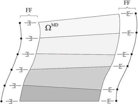
Figure 1. Traditional Free-Field (FF) boundaries and a two-dimensional (2D) main domain (MD) ${\mathrm{\Omega }}^{\text{MD}}$.

3 Finite element discretization

Considering the principle of virtual work (i.e., $\mathrm{\Pi }={\mathrm{W}}^{\text{int}}-{\mathrm{W}}^{\text{ext}}$), the implicit equilibrium equation is

$\begin{array}{cc}\hfill \mathrm{\Pi }=\frac{1}{2}{\int }_{\text{V}}\hfill & \hfill {\dot{\mathbf{ϵ}}}^{\text{T}}\mathbf{D}\mathbf{ϵ}\mathrm{d}\mathrm{V}-{\int }_{\text{V}}{\dot{\mathbf{u}}}^{\text{T}}\rho \left(\vec{\mathbf{b}}-\vec{\mathbf{a}}\right)\mathrm{d}\mathrm{V}\hfill \\ \hfill \hfill & \hfill -{\int }_{\mathrm{\Gamma }}{\dot{\mathbf{u}}}^{\text{T}}{\vec{\mathrm{\tau }}}^{\text{FF}}\mathrm{d}\mathrm{\Gamma }=0\hfill \end{array}(4)$

where $\mathbf{D}$ is the stiffness matrix, $\mathbf{ϵ}$ is the vector of incremental strains, $\mathbf{b}$ is the vector of body forces, $\mathbf{a}$ is the vector of accelerations, $\dot{\mathbf{u}}$ and $\dot{\mathbf{ϵ}}$ are the kinematically admissible continuous displacement and strain fields (i.e., virtual displacements and strains), and V and $\mathrm{\Gamma }$ are the body volume and boundary, respectively. Note that the FF term appears in the equilibrium equation as the body boundary traction. Then, by following standard finite element discretization procedures and considering $\mathrm{\Pi }=0$ (i.e., the sum of the internal, external, and inertial forces is equal to zero for any admissible virtual displacement), the equation of equilibrium can be written in matrix notation as

$\mathbf{M}\bar{\mathbf{a}}+\mathbf{C}\bar{\mathbf{v}}+\mathbf{K}\mathrm{\Delta }\bar{\mathbf{u}}={\mathbf{F}}^{\text{ext}}-{\mathbf{F}}^{\text{int}}-{\mathbf{F}}^{\text{FF}}(5)$

where $\mathbf{M}$, $\mathbf{C}$, and $\mathbf{K}$ are the mass, damping, and stiffness matrices, respectively; $\bar{\mathbf{a}}$, $\bar{\mathbf{v}}$, and $\bar{\mathbf{u}}$ are the acceleration, velocity, and displacement nodal vectors, respectively; and ${\mathbf{F}}^{\text{ext}}$, ${\mathbf{F}}^{\text{int}}$, and ${\mathbf{F}}^{\text{FF}}$ are the external, internal, and FF nodal force vectors, respectively. Note that: (1) the damping matrix $\mathbf{C}$ arises after including the velocity terms of Equation 1 in Equation 4; (2) by including the normal and shear tractions of Equation 1 in Equation 4, the corresponding local stiffness term must be added to the global stiffness matrix $\mathbf{K}$; (3) an extra load vector coming from the earthquake acceleration (i.e., ${\mathbf{F}}^{\text{eq}}=\mathbf{m}{\bar{\mathbf{a}}}^{\text{eq}}$, where eq denotes earthquake acceleration) can be added to Equation 5; (4) Equation 5 can be expressed as a function of time using a time integration scheme (e.g., Newmark, 1959); and (5) in Equation 5, $\bar{\mathbf{v}}$ at the boundary nodes is computed as

$\bar{\mathbf{v}}=\left(\frac{\partial {\bar{\mathbf{u}}}^{\text{FF}}}{\partial t}-\frac{\partial {\bar{\mathbf{u}}}^{2\text{D}}}{\partial t}\right)(6)$

in which Equation 6 is the difference in velocities between the corresponding boundary nodes of the 2D domain and the FF columns.

For the case in which an additional damping term is needed (e.g., Rayleigh damping), this must be added to Equation 5. The reader is directed to Nielsen (2006), Nielsen, (2014) for details of the terms concerning the FF formulation and their coupling with the 2D domain, and to Bathe (1996) and González Acosta (2020) for the FE matrix formulation and time stepping techniques.

4 Performance of dynamic boundaries

To evaluate the performance of standard dynamic boundaries, 1D columns, composed of both simple and ANCM materials, are used. These columns have dimensions of height h = 10 m and width w = 2 m, and are modelled using square, nine-noded plane strain elements. Each element has a side length of 1 m, resulting in columns comprising 10 by 2 elements, and each element uses $3\times 3$ Gauss integration points. It is important to note that, because these 1D columns are constructed using square elements, their behaviour is that of a 2D column (i.e., including rotational effects). Hence, special dynamic boundaries (either TD or FF) are required. The ANCM material is simulated using the material properties in Table 1, which are the properties of Hochstetten sand for a hypoplastic description with intergranular strains (Niemunis and Herle, 1997), as calibrated by Mašín (2019). In contrast, the simplified material is fully elastic, with the elastic properties being initialised via the hypoplastic model (that is, the initial elastic properties are computed using the hypoplastic model and are kept constant during the simulation). In the analysis of the column benchmarks in this section and Section 5, as well as the subsequent asymmetric benchmark in Section 6, a Rayleigh damping of $\zeta$ = 5% (corresponding to $\alpha$ = 0.4712 ${\text{s}}^{-1}$ and $\beta$ = 0.003978 s, where $\alpha$ and $\beta$ are the coefficients associated with the mass and stiffness matrices in $\mathbf{C}$ = $\alpha \mathbf{M}$ + $\beta \mathbf{K}$) has been implemented. Note that the Rayleigh damping coefficients are computed using $\alpha =2\zeta {\omega }_a{\omega }_b/({\omega }_a+{\omega }_b)$ and $\beta =2\zeta /({\omega }_a+{\omega }_b)$, where ${\omega }_a=6.28$ rad/s and ${\omega }_b=18.84$ rad/s. Furthermore, the material’s specific gravity, $G_s=2.65$, an initial void ratio, $e_0=0.75$, and a lateral earth pressure coefficient, $K_0=0.5$, are used to initialise the stresses (no pore water pressures are considered in this study). The earthquake is simulated using the 1999 Chi-Chi acceleration (component-0, station CWB CHY074 recorded at 29.3 km from the hypocentre), considering a 10-s time window between 10 and 20 s. Furthermore, it is assumed that the column is situated on a rigid bedrock, and the input earthquake loading has been amplified by a factor of 2, reaching a peak ground acceleration of 3.15 m/s², in order to exacerbate the detrimental boundary effects. Note that the input earthquake accelerations have not been subjected to a baseline correction, in order to enhance the replicability of results without introducing additional processing steps. Furthermore, it has been demonstrated that such a correction does not influence significantly the PGA values (Boore, 1999). Finally, in addition to the use of FF boundaries (the mathematical background of which was described in the previous section) for analysing the 1D column, TD boundaries have been incorporated into the series of analyses for comparative purposes. TD can be incorporated into the FEM formulation by duplicating the degrees of freedom of boundary nodes on one side of the domain (either left or right) with respect to the opposite side, thereby ensuring the (numerical) periodicity of the domain. A comprehensive description of this technique can be found in Cook et al. (1989).

Table 1

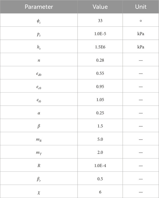
Table 1. Material properties for Hochstetten sand [after Mašín (2019)].

Figure 2 shows a sketch of the column deformed due to the applied earthquake load and indicates the locations at which the accelerations (surface) and stress paths (points A and B) were measured. Also, the ${\mathrm{V}}_{\mathrm{s}}$ profile (as initialised via the hypoplastic model) and the earthquake input (Center for Engineering Strong Motion Data, 1999) are depicted. Based on these initial data, the results corresponding to the fully elastic column in combination with TD and FF boundaries were obtained. Figures 3a, b show that the computed accelerations at the column surface, and their associated Fourier spectra, are nearly equal. Moreover, both computed results are close to reference (1D elastic) solution. This indicates that FF can simulate the (infinite) far-field via the application of lateral damping-loads, and any anomaly between the FF and the 2D domain can be corrected. Furthermore, the lack of advanced cyclic characteristics of the material prevents any (artificial) strength degradation and accumulation of (plastic) strains.

Figure 2

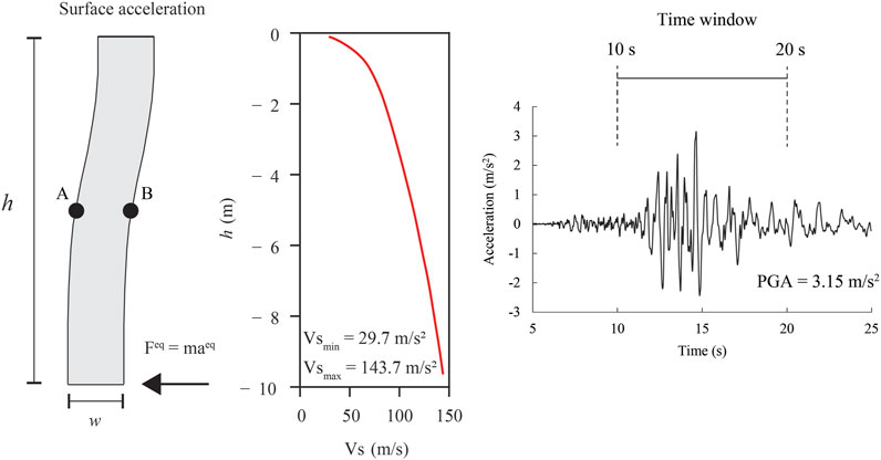
Figure 2. 1D elastic benchmark (left, not to scale), ${\mathrm{V}}_{\mathrm{s}}$ distribution (middle) and ground acceleration input (right). Acceleration data modified from Center for Engineering Strong Motion Data (1999).

Figure 3

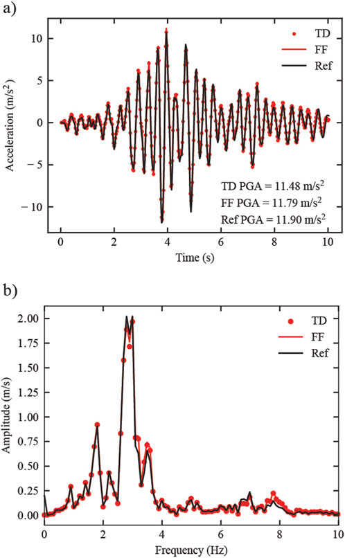
Figure 3. 1D elastic column (a) surface accelerations, and (b) Fourier spectra computed from the surface accelerations.

The anomaly between the FF and the 2D domain is demonstrated in Figure 4. Here, the 1D elastic column, at time t = 5 s (from the start of the time window in Figure 3a), undergoes a time-step increment, and hence an increment of load. At the end of the first equilibrium iteration (k = 1), unequal shear stresses are computed on either side of the column. Then, due to the FF loads, the column position is corrected through successive iterations (Figures 4a–e) until the shear stress distribution is approximately the same as in the FF. The stress correction as function of the iteration number is plotted in Figures 4f, g, in which the shear stresses at points A and B are shown, along with numbers (next to the data points) indicating the relative error $|{\tau }_k-{\tau }_{\text{final}}|/|{\tau }_{\text{final}}|$, where $\tau$ is the shear stress. Clearly, at the start of the first iteration (k = 0), the stresses at points A and B are opposite and far from the reference FF stress. Then, through the iterative process, the discrepancy is corrected. This obvious discrepancy is not a significant hindrance with elastic materials since no degradation occurs. However, when ANCMs are used, this discrepancy has a major effect on the results.

Figure 4

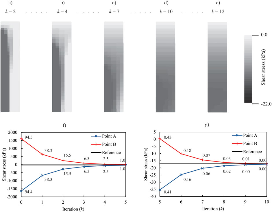
Figure 4. Shear stress distribution in the elastic column through successive iterations (k) of a typical time step: (a) k = 2, (b) k = 4, (c) k = 7, (d) k = 10, and (e) k = 12; and the shear stresses at points A and B throughout the iterative process, (f) k = 0 to k = 5, and (g) k = 5 to k = 10. Note that the contour range for shear stress refers only to the situation at k = 12.

Figure 5 shows the same benchmark with the results in terms of stresses, accelerations, Fourier spectra, and displacements when an ANCM is considered. Figure 5a shows the unevenly distributed vertical stresses in the 1D column next to the stresses of the FF columns at the end of the earthquake. This incongruous distribution of stresses is caused by the continuous adjustment between the soil column and the FF boundaries during the equilibrium iterations, triggering multiple artificial cyclic degradation mechanisms despite the symmetric arrangement of the benchmark. Note that the stress variation at a particular level in the column corresponds to the stress at each Gauss point, which in the case of two (laterally) connected square elements corresponds to 6 Gauss points in a row. Figures 5b, c respectively present the accelerations at the top of the column and their associated Fourier spectra, demonstrating that the TD and FF simulations produce highly comparable results. Nevertheless, it is observed that, when FF are used, the computed peak ground acceleration is 26% greater than that obtained using TD. As a consequence of this amplification, a similar response is observed in the Fourier spectrum, with a peak FF response 5.8% greater than that obtained using TD. Figure 5d shows the column settlement due to material compaction. With TD, the column deforms vertically by almost 0.13 m, whereas with FF boundaries the column is unable to deform. This is because FF loads fail to ensure a realistic idealisation of an infinite domain and are therefore unable to guarantee a realistic vertical movement of the 2D domain. Furthermore, Figures 6a, b illustrate the shear stress versus shear strain paths for points A and B throughout the earthquake. It is observed that, with TD, the shear waves propagate uniformly through the column, leading to identical outcomes at points A and B. Conversely, with the use of FF boundaries and considering an ANCM, the lateral support from FF proves insufficient for ensuring uniform shear wave transmission. Consequently, the performance of both boundaries varies significantly. Notably, points A and B diverge in their response paths, with point B exhibiting a substantial increase in strain magnitude, which accelerates the column’s degradation. This set of results shows that, although the ground accelerations obtained using FF are not that different from those obtained using TD, material degradation and continuous vertical deformation cannot be simulated accurately when FF are used. This is a significant limitation that impedes confidence in dynamic simulations when FF are used.

Figure 5

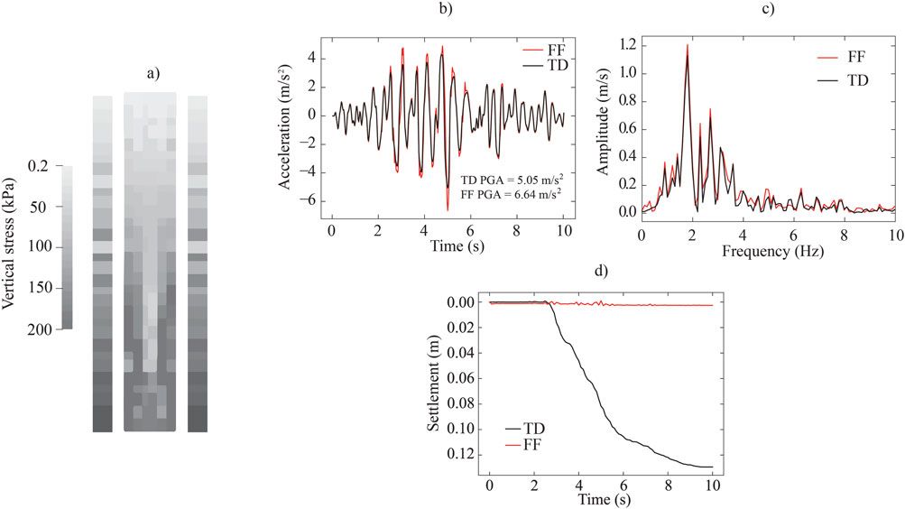
Figure 5. (a) Vertical stresses in the 1D column at the end of the earthquake considering FF and an ANCM, (b) accelerations at the column surface, (c) the respective Fourier spectra, and (d) column settlements.

Figure 6

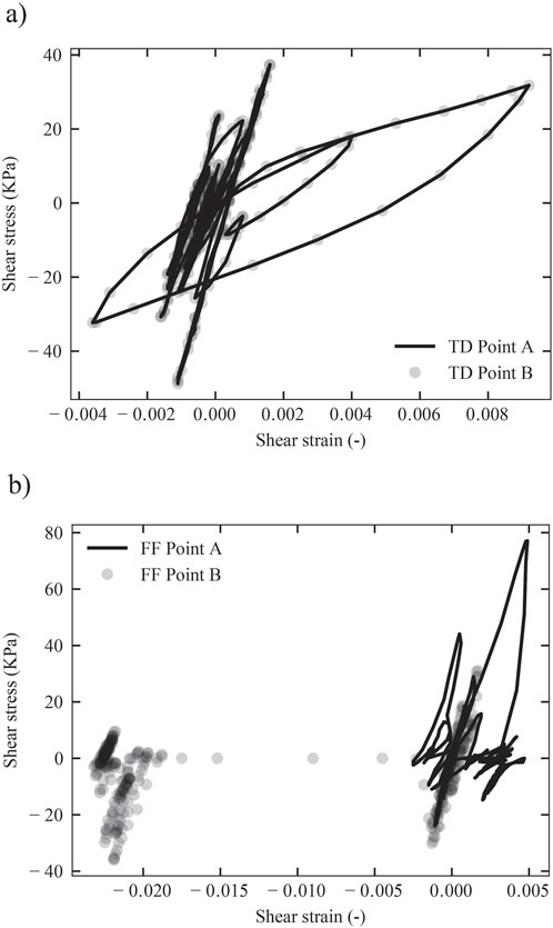
Figure 6. Stress–strain paths at points A and B in combination with an ANCM when (a) TD are used, and (b) FF are used.

5 Tied Free-Fields

The Tied Free-Field (TFF) concept combines the TD and FF methods by implementing traditional FF and tying the corresponding FF and 2D domain boundary nodes. Based on the premise that FF are numerically independent of the 2D domain, they can be solved in advance for each iteration of each time increment. After the nodal displacements of the FF are computed in the iteration step, these displacements are tied to the 2D domain boundary nodes by adding a large “penalty” term (Smith et al., 2013) to the relevant diagonal terms of the stiffness matrix of the 2D domain. Hence, each nodal displacement of the FF is associated with the corresponding boundary node in the 2D domain, thus prescribing FF displacement values to the 2D domain boundaries during the solution of Equation 5 (that is, Equation 5 is solved for the 2D domain considering the nodal displacements at the boundaries as boundary conditions). This technique guarantees an accurate transmission of the seismic waves from the FF to the 2D domain without anomalies. Figure 7 illustrates the steps followed when TFFs are implemented. Figure 7a shows the initial FEM setting, in which an external seismic load has been applied to the base of the FF column. Note that some nodes of the 2D domain boundary have been coloured in red, highlighting those nodes which are modified with the “penalty” term. Figure 7b shows the displacement (from $\mathrm{\Delta }{\mathrm{\delta }}_{\mathrm{a}}^{\mathrm{F}\mathrm{F}}$ to $\mathrm{\Delta }{\mathrm{\delta }}_{\mathrm{d}}^{\mathrm{F}\mathrm{F}}$) of the FF column due to the external load. Finally, Figure 7c shows the displacement of the 2D boundary nodes (from $\mathrm{\Delta }{\mathrm{\delta }}_{\mathrm{a}}^{\mathrm{2}\mathrm{D}}$ to $\mathrm{\Delta }{\mathrm{\delta }}_{\mathrm{d}}^{\mathrm{2}\mathrm{D}}$), and thus the displacement of the full 2D domain, as a result of the FF nodes being tied to the 2D boundary nodes. Note that, since FF are numerically independent of the 2D domain, asymmetric boundaries do not imply an additional complication and the solution procedure remains the same. Also, while this paper focuses on two-dimensional (2D) analyses due to their computational efficiency and widespread application in engineering practice, it is acknowledged that three-dimensional (3D) analyses offer a more comprehensive understanding of geotechnical behaviour under seismic loading. Although 3D implementations are not examined here, similar to the implementation of TD and FF boundaries in a 3D context, Tied Free-Fields can also be implemented by following the steps delineated in Figure 7. Finally, the benchmarks in this paper use a penalty value of $1.0\times 10^{10}$ kN/m. Note that this chosen value is based on the element stiffness; i.e., an appropriate penalty term is selected to ensure numerical stability. Background theory and examples on implementing the “penalty” strategy in FEM formulations can be found in Bathe (1996) and Smith et al. (2013).

Figure 7

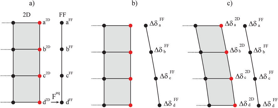
Figure 7. Steps followed in the TFF approach. (a) Application of the earthquake loading $({\mathrm{F}}^{\mathrm{e}\mathrm{q}})$ to the FF column, (b) deformation of the FF column, and (c) solution of Equation 5 considering the prescription of FF nodal displacements $(\mathrm{\Delta }{\mathrm{\delta }}^{\mathrm{F}\mathrm{F}})$ to the 2D domain boundary nodes $(\mathrm{\Delta }{\mathrm{\delta }}^{\mathrm{2}\mathrm{D}})$

To demonstrate the performance of TFF, the 1D column benchmark is tested again using the geometry and accelerations indicated in Figure 2 and the nonlinear material properties used in the Figure 5 benchmark. The settlements at the centre of the column (indicated by a red marker in Figures 8a–c) are recorded, while the width w is increased. Additionally, the computational time for each simulation, normalized by the time required for the TFF analysis (${\mathrm{t}}_n$), is included in the plots in Figure 8d to illustrate the relative computational cost. Figures 8b, c show that, when TD and TFF are used, the same final settlement is obtained despite considering a small width w. However, when FF are used (Figure 8a), the domain width must be substantially increased to reach a reasonable settlement at the centre of the domain. This is more evident in Figure 8d, where the increase of settlement with time is plotted. It is seen that TD and TFF give the same results even with w = 2 m. On the other hand, when FF are used, the column width must be increased to almost w = 20 m in order to reach a similar settlement (at the centre) as TD and TFF. Figure 9 shows the stress versus strain paths at points A and B when TFF are used. As observed, the results are virtually the same as those obtained when TD are used. The results shown in Figures 8, 9 again demonstrate the limitation of using FF boundaries and illustrate the advantages of using TFF for simple 1D seismic simulations.

Figure 8

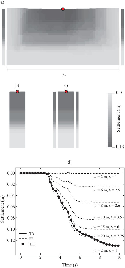
Figure 8. Settlements of the 2D domain using (a) FF, (b) TD, (c) TFF, and (d) comparison as a function of time and w.

Figure 9

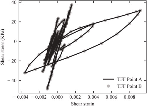
Figure 9. Stress–strain paths at points A and B when TFF are used in combination with an ANCM.

6 Asymmetric validation

To examine further the accuracy of TFF, the asymmetric problem in Figure 10 is analysed. It comprises a two-layer domain of h = 10 m and w = 30 m, with the lower layer being a linear elastic material and the upper layer being a sandy material modelled with the ANCM introduced above. Points A, B, and C were chosen to compare the results obtained using the different boundary conditions. Point A is located at the centre of the domain and points B and C are located 1 m away from each of the domain’s vertical boundaries. Since TD should only be applied when the boundaries of the domain are identical, a mirroring procedure has been imposed (dotted lines in Figure 10) to ensure equal properties at the lateral boundaries, thereby permitting the implementation of TD. The properties of the sandy material are the same as in the benchmark of Figure 5, and the properties of the elastic material are a Young’s modulus of $E=2.5\times \mathrm{1}{\mathrm{0}}^{\mathrm{5}}$ kPa and a Poisson’s ratio of $\nu =\mathrm{0.28}$. In contrast to the analysis in Section 5, the energy release at the ground surface is computed in addition to settlements. The energy release is analysed in terms of the ground response spectrum, which is the collection of a range of oscillating single-degree-of-freedom systems, each with a specific period $T$, in which the maximum acceleration is depicted as the spectral acceleration $(S_a)$. The response spectrum plots have been generated assuming a 5% damping ratio. Furthermore, they have been normalised by the maximum ground acceleration $(a_{\mathit{max}})$ obtained at the respective analysed locations.

Figure 10

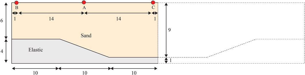
Figure 10. Asymmetric benchmark (not to scale and dimensions in meters).

Figure 11 shows the spatial distribution of settlements at the end of the earthquake. It is observed that the settlements are similar when TD and TFF boundaries are used. On the other hand, analogous to the results obtained in the 2D benchmark of Figure 8, the settlement profile does not describe the desired vertical deformation at the boundaries when using FF. Although the true settlement profile is difficult (if not impossible) to know via simulations, the consistent settlement distribution (with respect to the geometry of the elastic part of the domain), computed using TFF, indicates that the performance of this boundary condition is comparable to TD (after adjustment of the domain size) and superior to FF boundaries. Figure 12 shows the detailed behaviour at point A. Figures 12a, b show similar behaviour in terms of settlements, and almost identical behaviour in terms of energy released, when FF and TFF are used. This demonstrates again that TFF can yield similar results to traditional FF when the measurement location is far from the boundaries. In contrast, when TD are used, the settlements and energy released are noticeably reduced, indicating that replacement of the FF columns (those along the left and right edges of the domain in Figures 11b, c) by a larger domain employing tied boundaries can lead to a reduced flow of energy to the centre of the domain.

Figure 11

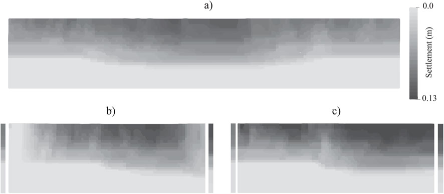
Figure 11. Settlements obtained at the end of the earthquake using (a) TD, (b) FF, and (c) TFF.

Figure 12

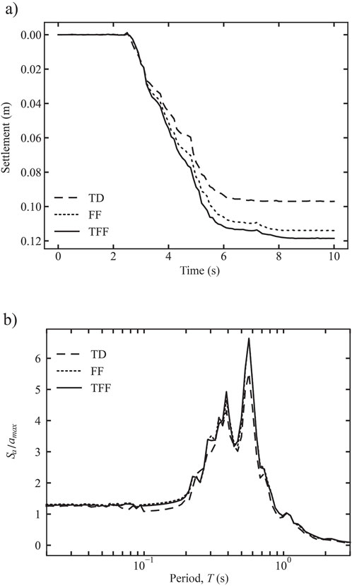
Figure 12. (a) Settlements during the earthquake, and (b) response spectra computed using the ground accelerations at point A.

Figures 13, 14 show the results obtained at the edges of the TD, FF and TFF domains. These sets of results are of high relevance since at these points (i.e., points B and C) the effect of the boundary is significant, hence providing evidence about the effectiveness of one approach over another. Furthermore, the responses of 1D isolated columns using the material distributions at each vertical boundary, which represent the far-field responses at the left and right edges of the domain, have been included in the plots and are designated as the “reference solution”. In terms of settlements, Figure 13a shows that FF boundaries fail to reproduce the compaction of the material due to earthquake loading, whereas TFF predicts significant settlements and TD yields results closer to the reference solution. With respect to energy release, Figure 13b shows that, at the points of higher response amplitude ($\approx$ 0.3 s and 0.5 s), the TD and the FF results under- and over-estimate the reference solution, respectively. In contrast, the TFF results remain relatively close to the reference solution.

Figure 13

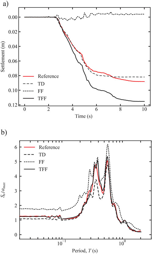
Figure 13. (a) Settlements during the earthquake, and (b) response spectra computed using the ground accelerations at point B.

Figure 14

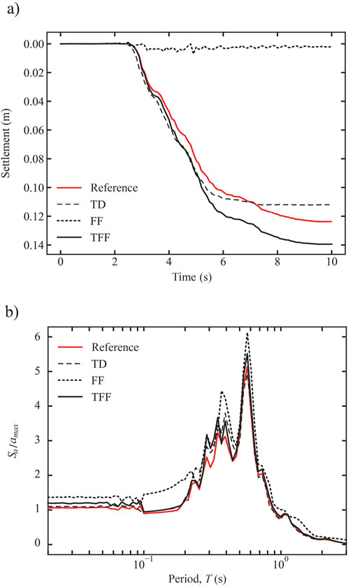
Figure 14. (a) Settlements during the earthquake, and (b) response spectra computed using the ground accelerations at point C.

Finally, Figure 14 shows the results at the centre of the domain when TD are used and at the right edge of the domain when FF and TFF boundaries are used. As with all results computed at the domain edges, the FF boundaries fail to predict an adequate vertical deformation, whereas the TD and TFF boundaries produce results closer to the reference solution (Figure 14a). Additionally, traditional FF boundaries again produce an upper bound to the energy released, while TD and TFF yield results similar to those obtained from the reference solution (Figure 14b). In conclusion, when ANCM are used, TFF and TD boundaries offer a reasonable approximation to the reference solution, in comparison to FF. However, it is important to remember that essential adjustments are needed for TD, such as the mirroring procedure used in this asymmetric benchmark. The improved results obtained when using TFF, which are particularly evident in the behavior of points B and C in comparison to the reference solution, serve as a robust testament to the effectiveness of this approach in simulating boundary behavior in earthquake-related problems.

7 Discussion

Throughout this paper, the effectiveness of the proposed method, Tied Free-Fields, has been demonstrated through various benchmarks. However, it is acknowledged that a more comprehensive investigation, exploring a wider range of material properties, mesh sizes, damping ratios, and domain variations under diverse conditions, would further strengthen the assessment of the method’s accuracy and applicability. In particular, the following aspects may be explored:

• Constitutive laws: While the method has been tested with the hypoplastic model incorporating intergranular strain, a wide range of constitutive laws is used in practice. To fully demonstrate its capabilities, the method should be tested with the most commonly used constitutive laws.

• Saturation effects: The method has been tested under dry conditions. Extending the method to account for excess pore water pressures is an important step for future development.

8 Conclusion

This paper has proposed a new boundary condition for the application of earthquake loading, namely, Tied Free-Fields (TFF), with the aim of improving the accuracy and efficiency of seismic simulations. The results of earthquake simulations under elastic conditions indicate that TFF boundaries are capable of producing results comparable with those obtained with TD and FF boundaries. In contrast, when symmetric and non-symmetric conditions are considered in combination with advanced non-linear cyclic models (ANCMs), TFF boundaries are capable of producing results comparable with, and at times superior to, those obtained with Tied-Degree boundaries, and far superior to those obtained with Free-Field boundaries. It was found that TFF does not suffer from the significant boundary inaccuracies typically associated with traditional Free-Fields (FF). Moreover, the precision of TFF reduces the need for extended 2D (or 3D) domains to mitigate boundary effects, as is necessary with standard dynamic boundaries, leading to a more efficient use of computational resources. This suggests that the application of TFF in seismic simulations could substantially enhance both material behaviour analysis and energy release predictions.

Data availability statement

The raw data supporting the conclusions of this article will be made available by the authors, without undue reservation.

Author contributions

JG: Conceptualization, Formal Analysis, Investigation, Methodology, Validation, Visualization, Writing–original draft. AV: Supervision, Writing–review and editing. MH: Funding acquisition, Project administration, Supervision, Writing–review and editing.

Funding

The author(s) declare that financial support was received for the research and/or publication of this article. The results presented in the paper are part of the research programme DeepNL/SOFTTOP with project number DEEP.NL.2018.006, financed by the Netherlands Organisation for Scientific Research (NWO).

Conflict of interest

The authors declare that the research was conducted in the absence of any commercial or financial relationships that could be construed as a potential conflict of interest.

Generative AI statement

The author(s) declare that no Generative AI was used in the creation of this manuscript.

Publisher’s note

All claims expressed in this article are solely those of the authors and do not necessarily represent those of their affiliated organizations, or those of the publisher, the editors and the reviewers. Any product that may be evaluated in this article, or claim that may be made by its manufacturer, is not guaranteed or endorsed by the publisher.

References

Barrero, A. R., Taiebat, M., and Lizcano, A. (2015). “Application of an advanced constitutive model in nonlinear dynamic analysis of tailings dam,” in GEOQuebec (Quebec), 20–23.

Google Scholar

Basu, D., Montgomery, J., and Stuedlein, A. W. (2022). Observations and challenges in simulating post-liquefaction settlements from centrifuge and shake table tests. Soil Dyn. Earthq. Eng. 153, 107089. doi:10.1016/j.soildyn.2021.107089

CrossRef Full Text | Google Scholar

Basu, U., and Chopra, A. K. (2003). Perfectly matched layers for time-harmonic elastodynamics of unbounded domains: theory and finite-element implementation. Comput. Methods Appl. Mech. Eng. 192, 1337–1375. doi:10.1016/s0045-7825(02)00642-4

CrossRef Full Text | Google Scholar

Bathe, K. J. (1996). Finite element procedures. New Jersey: Prentice Hall.

Google Scholar

Benz, T. (2007). Small-strain stiffness of soils and its numerical consequences. Germany: University of Stuttgart. Ph.D. thesis.

Google Scholar

Bettess, P. (1977). Infinite elements. Int. J. Numer. Methods Eng. 11, 53–64. doi:10.1002/nme.1620110107

CrossRef Full Text | Google Scholar

Bielak, J., and Loukakis, K. (2025). A note on the implementation of the effective seismic input for the domain reduction method. Bull. Seismol. Soc. Am. doi:10.1785/0120240171

CrossRef Full Text | Google Scholar

Bielak, J., Loukakis, K., Hisada, Y., and Yoshimura, C. (2003). Domain reduction method for three-dimensional earthquake modeling in localized regions, Part I: Theory. Bull. Seismol. Soc. Am. 93, 817–824. doi:10.1785/0120010251

CrossRef Full Text | Google Scholar

Boore, D. M. (1999). Effect of baseline corrections on response spectra for two recordings of the 1999 Chi-Chi, Taiwan, earthquake (Open-File Report 99-545, Version 1.0). US Geological Survey.

Google Scholar

Budimir, M. E. A., Atkinson, P. M., and Lewis, H. G. (2014). Earthquake-and-landslide events are associated with more fatalities than earthquakes alone. Nat. Hazards 72, 895–914. doi:10.1007/s11069-014-1044-4

CrossRef Full Text | Google Scholar

Center for Engineering Strong Motion Data (1999). Available online at: https://www.strongmotioncenter.org/vdc/scripts/stnpage.plx?stations=2327 (Accessed June, 2023).

Google Scholar

Chapel, F. (1987). Boundary element method applied to linear soil–structure interaction on a heterogeneous soil. Earthq. Eng. Struct. Dyn. 15, 815–829. doi:10.1002/eqe.4290150703

CrossRef Full Text | Google Scholar

Clayton, R., and Engquist, B. (1977). Absorbing boundary conditions for acoustic and elastic wave equations. Bull. Seismol. Soc. Am. 67, 1529–1540. doi:10.1785/bssa0670061529

CrossRef Full Text | Google Scholar

Cook, R. D., Malkus, D. S., and Plesha, M. E. (1989). Concepts and applications of finite element analysis. New York: John Wiley and Sons.

Google Scholar

Davoodi, M., Pourdeilami, A., Jahankhah, H., and Jafari, M. K. (2018). Application of perfectly matched layer to soil-foundation interaction analysis. J. Rock Mech. Geotech. Eng. 10, 753–768. doi:10.1016/j.jrmge.2018.02.003

CrossRef Full Text | Google Scholar

Do, P. C., Vardon, J. P., González Acosta, J. L., and Hicks, M. A. (2022). “Implementing dynamic boundary conditions with the material point method,” in 16th IACMAG (Torino), 221–228.

Google Scholar

Galavi, V., Petalas, A., and Brinkgreve, R. B. J. (2013). Finite element modelling of seismic liquefaction in soils. Geotech. Eng. J. SEAGS and AGSSEA 44, 55–64. doi:10.14456/seagj.22013.21

CrossRef Full Text | Google Scholar

González Acosta, J. L. (2020). Investigation of MPM inaccuracies, contact simulation and robust implementation for geotechnical problems. Netherlands: Delft University of Technology. Ph.D. thesis.

Google Scholar

González Acosta, J. L., van den Eijnden, A. P., and Hicks, M. A. (2022). “Liquefaction assessment and soil spatial variation,” in 16th IACMAG (Torino), 283–290.

Google Scholar

Hagstrom, T., and Warburton, T. (2004). A new auxiliary variable formulation of high-order local radiation boundary conditions: corner compatibility conditions and extensions to first-order systems. Wave Motion 39, 327–338. doi:10.1016/j.wavemoti.2003.12.007

CrossRef Full Text | Google Scholar

Hu, D., Li, F., Zhang, L., and Zhang, K. (2020). An advanced absorbing boundary for wave propagation analysis in saturated porous media. Soil Dyn. Earthq. Eng. 136, 106204. doi:10.1016/j.soildyn.2020.106204

CrossRef Full Text | Google Scholar

Kellezi, L. (1998). Dynamic soil-structure interaction transmitting boundary for transient analysis. Denmark: Technical University of Denmark. Ph.D. thesis.

Google Scholar

Kontoe, S. (2006). Development of time integration schemes and advanced boundary conditions for dynamic geotechnical analysis. United Kingdom: Imperial College London. Ph.D. thesis.

Google Scholar

Kontoe, S., Zdravkovic, L., and Potts, D. (2009). An assessment of the domain reduction method as an advanced boundary condition and some pitfalls in the use of conventional absorbing boundaries. Int. J. Numer. Anal. Methods Geomech. 33, 309–330. doi:10.1002/nag.713

CrossRef Full Text | Google Scholar

Li, Y., Zhao, M., Xu, C., Du, X., and Li, Z. (2018). Earthquake input for finite element analysis of soil-structure interaction on rigid bedrock. Tunn. Undergr. Space Technol. 79, 250–262. doi:10.1016/j.tust.2018.05.008

CrossRef Full Text | Google Scholar

Liu, H., Abell, J. A., Diambra, C., and Pisanò, F. (2019). Modelling the cyclic ratcheting of sands through memory-enhanced bounding surface plasticity. Géotechnique 69, 783–800. doi:10.1680/jgeot.17.p.307

CrossRef Full Text | Google Scholar

Luque, R., and Bray, J. D. (2020). Dynamic soil-structure interaction analyses of two important structures affected by liquefaction during the Canterbury earthquake sequence. Soil Dyn. Earthq. Eng. 133, 106026. doi:10.1016/j.soildyn.2019.106026

CrossRef Full Text | Google Scholar

Lysmer, J., and Kuhlemeyer, R. L. (1969). Finite dynamic model for infinite media. J. Eng. Mech. Div. (ASCE) 95, 859–877. doi:10.1061/jmcea3.0001144

CrossRef Full Text | Google Scholar

Mansur, W. J. (1983). A time stepping technique to solve wave propagation problems using the boundary element method. United Kingdom: University of Southampton. Ph.D. thesis

Google Scholar

Manzari, M. T., and Dafalias, Y. F. (2015). A critical state two-surface plasticity model for sands. Géotechnique 47, 255–272. doi:10.1680/geot.1997.47.2.255

CrossRef Full Text | Google Scholar

Mašín, D. (2019). Modelling of soil behaviour with hypoplasticity: Another approach to soil constitutive modelling. AG Switzerland: Springer Cham.

Google Scholar

Medicus, G., Tafili, M., Bode, M., Fellin, W., and Wichtmann, T. (2023). Clay hypoplasticity coupled with small-strain approaches for complex cyclic loading. Acta Geotech. 19, 631–650. doi:10.1007/s11440-023-02087-w

PubMed Abstract | CrossRef Full Text | Google Scholar

Modaressi, H., and Benzenati, I. (1992). “An absorbing boundary element for dynamic analysis of two-phase media,” in 10th world conf. Earthq. Eng, 1157–1163.

Google Scholar

Newmark, N. M. (1959). A method of computation for structural dynamics. J. Eng. Mech. Div. (ASCE) 85, 67–94. doi:10.1061/jmcea3.0000098

CrossRef Full Text | Google Scholar

Nielsen, A. H. (2006). “Absorbing boundary conditions for seismic analysis in ABAQUS,” in ABAQUS users’ conference (Boston), 359–376.

Google Scholar

Nielsen, A. H. (2014). Towards a complete framework for seismic analysis in ABAQUS. Proc. Inst. Civ. Eng. - Eng. Comput. Mech. 167, 3–12. doi:10.1680/eacm.12.00004

CrossRef Full Text | Google Scholar

Niemunis, A., and Herle, I. (1997). Hypoplastic model for cohesionless soils with elastic strain range. Mech. Cohes.-Frictional Mater. 2, 279–299. doi:10.1002/(sici)1099-1484(199710)2:4<279::aid-cfm29>3.0.co;2-8

CrossRef Full Text | Google Scholar

Paull, N., Boulanger, R. W., and DeJong, J. T. (2020). Accounting for spatial variability in nonlinear dynamic analyses of embankment dams on liquefiable deposits. J. Geotech. Geoenviron. Eng. (ASCE) 146, 04020124. doi:10.1061/(asce)gt.1943-5606.0002372

CrossRef Full Text | Google Scholar

Pretell, R., Ziotopoulou, K., and Davis, C. A. (2021). Liquefaction and cyclic softening at Balboa Boulevard during the 1994 Northridge earthquake. J. Geotech. Geoenviron. Eng. (ASCE) 147, 05020014. doi:10.1061/(asce)gt.1943-5606.0002417

CrossRef Full Text | Google Scholar

Prevost, J. H. (1985). A simple plasticity theory for frictional cohesionless soils. Int. J. Soil Dyn. Earthq. Eng. 4, 9–17. doi:10.1016/0261-7277(85)90030-0

CrossRef Full Text | Google Scholar

Seequent (2023). PLAXIS: free field boundary conditions for PLAXIS 2D: new improvements and recommendations for practical use. (Technical Report). Seequent, The Bentley Subsurface Company.

Google Scholar

Seidalinov, G., and Taiebat, M. (2014). Bounding surface SANICLAY plasticity model for cyclic clay behavior. Int. J. Numer. Anal. Methods Geomech. 38, 702–724. doi:10.1002/nag.2229

CrossRef Full Text | Google Scholar

Semblat, J. F., Gandomzadeh, A., and Lenti, L. (2010). A simple numerical absorbing layer method in elastodynamics. C. R. Mécanique 338, 24–32. doi:10.1016/j.crme.2009.12.004

CrossRef Full Text | Google Scholar

Smith, I. M., Griffiths, D. V., and Margetts, L. (2013). Programming the finite element method. New Jersey: John Wiley and Sons.

Google Scholar

Smith, W. D. (1974). A nonreflecting plane boundary for wave propagation problems. J. Comput. Phys. 15, 492–503. doi:10.1016/0021-9991(74)90075-8

CrossRef Full Text | Google Scholar

Subasi, O., Koltuk, S., and Iyisan, R. (2022). A numerical study on the estimation of liquefaction-induced free-field settlements by using PM4Sand model. KSCE J. Civ. Eng. 26, 673–684. doi:10.1007/s12205-021-0719-0

CrossRef Full Text | Google Scholar

Torabi, H., and Rayhani, M. H. T. (2014). Three dimensional finite element modeling of seismic soil-structure interaction in soft soil. Comput. Geotech. 60, 9–19. doi:10.1016/j.compgeo.2014.03.014

CrossRef Full Text | Google Scholar

Xu, C., Song, J., Du, X., and Zhao, M. (2017). A local artificial-boundary condition for simulating transient wave radiation in fluid-saturated porous media of infinite domains. Int. J. Numer. Methods Eng. 112, 529–552. doi:10.1002/nme.5525

CrossRef Full Text | Google Scholar

Ye, J., and Wang, G. (2016). Numerical simulation of the seismic liquefaction mechanism in an offshore loosely deposited seabed. Bull. Eng. Geol. Environ. 75, 1183–1197. doi:10.1007/s10064-015-0803-0

CrossRef Full Text | Google Scholar

Zienkiewicz, O. C., Bicanic, N., and Shen, F. Q. (1989). “Earthquake input definition and the transmitting boundary conditions,” in Adv. Comput. Nonlinear Mech. (Springer-Verlag), 1183–1197.

Google Scholar

Ziotopoulou, K., and Boulanger, R. W. (2013). “Numerical modeling issues in predicting post-liquefaction reconsolidation strains and settlements,” in 10th CUEE (Tokyo), 469–475.

Google Scholar