Development of a site and motion proxy-based site amplification model for shallow bedrock profiles using machine learning

Accurate prediction of site amplification is crucial for seismic hazard assessment, particularly at shallow bedrock sites where limited data can constrain modeling efforts. Traditional regression-based models often fail to capture complex nonlinear interactions inherent in seismic ground response. This study aims to develop proxy-based linear and nonlinear site amplification models that provide reliable predictions using machine learning (ML) techniques, enabling practical applications in regional ground motion modeling. The outputs of a series of one-dimensional site response analyses were used for training. Three ML algorithms were used: random forest (RF), extreme gradient boosting (XGB), and deep neural network (DNN). The models incorporated four site proxies and two motion proxies to predict site amplification, and their performance was evaluated against both a conventional regression-based model and a rigorous ML model utilizing full shear-wave velocity profiles and input motion spectra. When identical proxies were used, the differences between the regression and ML-based models were not pronounced. However, when the ML model was trained simultaneously with the site and motion proxies for both linear and nonlinear components, the prediction performance was significantly enhanced. This revealed that the traditional two-track approach of the site-proxy-dependent linear component and motion-proxy-conditioned nonlinear component is ineffective. A pairing scheme for site and motion proxies is recommended to achieve the most accurate predictions. Among the three ML methods, the RF algorithm exhibited the weakest performance. The XGB and DNN algorithms’ prediction accuracies were superior to the RF algorithm. The XGB and DNN outperformed each other when predicting the linear and nonlinear components, respectively. The proposed ML models achieved coefficient of determination (R²) values up to 0.97 with root mean square error (RMSE) as low as 0.04 for linear components, and R² up to 0.92 with RMSE as low as 0.06 for nonlinear components, demonstrating significant improvements over conventional regression-based models. Compared with a rigorous ML model, the proxy-based models exhibited agreeable predictions with far less information, illustrating the benefit of adopting the ML algorithms for improved adaptability and predictive capability. The constraint imposed on the site type, considering only profiles with a bedrock depth of less than 30 m, may have resulted in the strong performance of the proxy-based model.

1 Introduction

Predicting earthquake hazards is essential to enhancing the resilience of urban societies. Various forms of ground motion models (GMMs) have been developed to estimate the ground motion intensity. The site amplification term is an important component of a GMM, developed from recorded data in regions where available (Choi and Stewart, 2005; Chiou and Youngs, 2008; Walling et al., 2008). In areas where recordings are lacking, site amplification is determined using one-dimensional (1D) site response analysis (SRA) (Harmon et al., 2019; Hashash et al., 2021). Various site proxies (SPs) are used in site amplification models. The time-averaged shear wave velocity (V_S) of the upper 30 m (V_S30) is the most important and widely used SP in GMM. Borcherdt (1994) introduced V_S30 as a key parameter for seismic site classification. Boore et al. (1997) quantified its influence on predicting ground motion amplitudes. Choi and Stewart (2005) highlighted regional variability in V_S30 values and its impact on GMMs. Walling et al. (2008) and Seyhan and Stewart (2014) further refined site amplification models incorporating V_S30. Sandıkkaya and Dinsever (2018) investigated the combined use of V_S30 with the depth at V_S reaches 1 km/s or greater (Z_1.0) for better site characterization. Harmon et al. (2019) emphasized the integration of multiple site proxies, including V_S30, site period (T_G), and depth to the bedrock (H) to enhance modeling accuracy. Aaqib et al. (2021) focused specifically on developing models for shallow bedrock conditions, confirming the central role of V_S30 in site amplification prediction. However, using only V_S30 is insufficient to capture site-specific amplification, as highlighted by several studies. Mucciarelli and Gallipoli (2006) emphasized that V_S30 alone may not adequately reflect the resonance characteristics of soft soil sites. Assimaki et al. (2008) demonstrated that local soil heterogeneities can significantly influence site response, which V_S30 cannot fully represent. Castellaro et al. (2008) argued for including additional proxies, such as T_G, to improve the prediction of site amplification. Kokusho and Sato (2008) reported discrepancies between measured and predicted amplifications when relying solely on V_S30. Lee and Trifunac (2010) pointed out that V_S30 does not effectively capture nonlinear site effects under strong ground motions. The H (Harmon et al., 2019), Z_1.0, (Chiou and Youngs, 2014; Sandıkkaya and Dinsever, 2018), and T_G (Harmon et al., 2019; Aaqib et al., 2021) have been utilized with V_S30 for improved predictions. The fundamental resonance frequency (f₀) and corresponding amplitude (A₀) of the horizontal-to-vertical spectral ratio (HVSR) have also been employed to predict site amplification (Héloïse et al., 2012).

Regression analyses were conducted to develop site amplification models using both SPs and motion proxies (MPs). While SPs and MPs have been widely used to characterize site amplification, regression-based models possess inherent limitations. These models are easy to implement but can only provide averaged or representative values, lacking the ability to capture complex site-specific variability. To overcome these limitations, researchers have increasingly adopted conventional machine learning (ML) algorithms as data-driven alternatives to improve predictive performance. Although such ML models have addressed some shortcomings of regression approaches, their predictive accuracy remains limited, particularly in modeling the complex, nonlinear interactions present in seismic data (Cheng and Ziotopoulou, 2023). These models, such as random forest (RF) and gradient boosting rely on hand-crafted features and often struggle to capture the complex, high-dimensional relationships inherent in seismic data. Wang et al. (2023) have successfully employed RF and XGB models to predict site amplification based on SPs and MPs. Similarly, Kim et al. (2020) applied ML algorithms including RF and XGB to develop ground motion amplification models for Japan, highlighting their applicability and limitations in capturing regional site effects. In contrast, advanced ML models, especially deep learning, have demonstrated a remarkable ability to automatically extract hierarchical features from recorded seismic signals, making them well-suited for modeling complex ground motion phenomena (Mousavi and Beroza, 2023). Several recent studies have successfully applied these methods to real-world scenarios. For example, Mousavi et al. (2020) proposed the Earthquake Transformer, a deep learning model capable of simultaneous event detection and phase picking, while Ma et al. (2024) demonstrated high-resolution seismic imaging using convolutional and transformer-based neural networks (NNs). Similarly, Zhang and Zhang (2024) developed a universal deep learning model for real-time earthquake early warning, trained on data from diverse tectonic environments. Agata et al. (2025) integrated physical constraints into NNs to quantify uncertainty in seismic velocity structure and hypocenter estimation. Building on these advancements, hybrid frameworks that combine conventional ML models with deep learning architectures have also emerged, aiming to leverage the strengths of both model types (Mousavi et al., 2024). These developments underscore the growing need to incorporate advanced ML models into site amplification prediction, where the inherent complexity and variability of seismic site conditions demand more flexible and powerful predictive tools.

Many studies have used ML models to predict site amplification using SPs and MPs. Derras et al. (2017) investigated the effect of SPs on the estimation of nonlinear site amplification using the Kiban–Kyoshin Network (KiK-net) database. An artificial neural network (ANN) structure was used to predict the peak motion intensities. The SPs used were V_S30, topographical slope, fundamental resonance frequency f₀, and the depth beyond which V_S exceeded 800 m/s (H₈₀₀). The results showed that the V_S30 and H₈₀₀ pairs were the most effective over short periods, whereas the f₀ and H₈₀₀ pairs performed most favorably over long periods. Stambouli et al. (2017) assessed the influence of SPs on the Fourier amplification factor (FAF) using outputs from 1D linear SRAs. A generalized regression NN was used to train and predict the FAFs. A case in which all SPs were used exhibited the lowest standard deviation, but the V_S30 and f₀ pairs were recommended for practical applications. Ilhan et al. (2019) predicted both linear and nonlinear site amplifications in Central and Eastern North America. The ANN model was trained using proxies identical to those used in a regression-based site amplification model (Harmon et al., 2019): V_S30, T_G, depth to weathered rock (Z_Soil), and peak ground acceleration (PGA). Derras et al. (2020) estimated the effects of soil nonlinearity on site responses using five SPs and seven MPs. They trained an ANN using 2,927 sets of recordings from the KiK-net database. Sensitivity analyses were performed using various combinations of SPs and MPs. The combination of the peak ground velocity (PGV)/V_S30, V_S30, and f₀ determined from the HVSR of surface earthquake recordings (f_0HV) provided the most favorable predictions. Only a single MP was used in each pairing, and the effect of training with multiple MPs was not considered. Furthermore, only the nonlinear component of site amplification was developed. Bergamo et al. (2021) used univariate regression and a NN to predict Fourier amplitudes based on Swiss and Japan databases. Sensitivity analyses were performed using different SP combinations. The application of quarter-wavelength velocity and impedance contrast pairing outperformed other combinations at all frequencies, whereas the use of V_S30 showed an acceptable match in the medium-frequency range.

Thus, the use of ML is gaining wide popularity for the development of site amplification models. Although one of the primary strengths of ML lies in its ability to operate with multiple proxies with different characteristics, previous studies followed the classical framework of using only SPs for linear amplification predictions. Improvement in performance using additional SPs relative to regression-based approaches has been a focus of interest. The effect of utilizing SPs and MPs for the prediction of both the linear and nonlinear components of site amplification has not been fully explored.

Additionally, research on the application of ML, specifically for the prediction of site amplification for shallow bedrock profiles, is still limited. Lee et al. (2023) used deep neural network (DNN) and RF algorithms to predict site amplification. Because the objective of the study was to evaluate whether the ML-based model could achieve sufficient accuracy to eventually replace a numerical model, inputs similar to those required in a 1D SRA were used for training. The inputs included the entire V_S profile and response spectrum of the input motion. Both the DNN and RF models produced an exceptional fit to the calculated responses. However, using this model in a GMM is difficult because the V_S profile must be specified as an input.

In this study, ML-based models were developed to predict shallow bedrock site amplification using only SPs and MPs. Because the objective was to develop a proxy-based model for application in a regional GMM, easily obtainable proxies were used as input data. Various pairings of SPs and MPs were tried to select the optimum combinations for both the linear and nonlinear site amplification components. We used several ML algorithms to evaluate which method yielded the most accurate predictions. The performances of the ML models were extensively compared with that of the regression-based model of Aaqib et al. (2021) The proxy-based ML models were also compared against the DNN model of Lee et al. (2023) trained with a full V_S profile and response spectrum.

2 Site response analysis database and regression-based site amplification model

2.1 Presentation of data

The outputs of linear and nonlinear SRAs reported by Aaqib et al. (2021) were used in this study. Aaqib et al. (2021) selected 40 measured Vs profiles as baseline soil columns. Because the objective of this study was to develop a site amplification model that can potentially be used in practice, conservative estimates of amplification were intended. Therefore, only profiles without stiffness reversal were selected because they could produce deamplification. Owing to the insufficient number of measured profiles, the baseline Vs profiles were randomized using the procedure proposed in Toro (1995), resulting in 840 V_S profiles. In performing the site response analyses, we used 51 recorded ground motions. The motions included recordings from regional earthquakes (2016 Gyeongju and 2017 Pohang events) as well as rock outcrop ground motions from the NGA-West2 database and the Nuclear Regulatory Guide (NUREG-6729). PGAs of the motion ranged from 0.01g to 0.5g.

Site response analyses were performed using the 1D SRA program DEEPSOIL v7 (DEEPSOIL, 2024). The shear modulus reduction and damping curves proposed by Darendeli (2001) were used as the reference nonlinear curves. The General Quadratic/Hyperbolic constitutive model of Groholski et al. (2016) and modulus reduction and damping curve-fitting procedures were applied. The target shear strength was calculated following the Mohr–Coulomb failure criterion. A total of 42,840 linear and nonlinear analyses were conducted with full combinations of 840 V_S profiles and 51 motions.

2.2 Reference regression-based site amplification model

A regression-based site amplification model was proposed by Aaqib et al. (2021) based on the outputs of SRAs. The amplification outputs comprise two components, defined as Equation 1:

$Amp\left(T\right)=F_{LIN}\left(T\right)+F_{NL}\left(T\right)(1)$

where T is the spectral period, Amp(T) is the total amplification, F_LIN(T) is the linear component, and F_NL(T) is the nonlinear component. In the following, the symbol T is omitted for simplicity. F_LIN was calculated by dividing the spectral acceleration (SA) at the surface by SA at the rock outcrop using the 1D linear SRA results. Amp was calculated by dividing SA at the surface by SA at the bedrock using the 1D nonlinear SRA results, whereas F_NL was calculated by subtracting F_LIN from Amp. Based on the outputs, predictive equations for F_LIN and F_NL were developed. For F_LIN, a predictive equation dependent on V_S30 was developed, denoted as (F_LIN)_Vs30. It can be used with an additive term conditioned on T_G to account for the effect of site resonance. This linear component is denoted as (F_LIN)_VS30+TG.

The F_NL equation is dependent on the motion proxy, PGA_rock, defined as Equation 2:

$F_{NL}=f_2\ln \left(\frac{{PGA}_{rock}+f_1}{f_1}\right)(2)$

where f₁ = 0.1 g and f₂ is a coefficient of the model. f₂ is conditioned on both T and V_S30 bins to account for the effect of site profile. This indirect procedure was used for F_NL due to difficulties in incorporating both site and motion proxies in a regression. These site amplification functional forms are hereafter referred to as the AEA21 model.

2.3 Reference ML-based site amplification model

DNN and RF-based site amplification models were developed by Lee et al. (2023) based on the identical outputs of SRAs, which is hereafter referred to as the LEA23 model. The LEA23 model used extensive set of information for training including 113 spectral accelerations of the input ground motion and the entire V_S profile (up to 29 layers) for training. The purpose for the development of the LEA23 model was to evaluate the possibility of reproducing the results of a 1D SRA, and hence similar resolution of input information was used. It can thus be considered as the rigorous model.

3 Machine learning models

Two tree-based algorithms, RF and extreme gradient boosting (XGB), and a DNN algorithm were used to predict site amplification. The basic principles of these algorithms are presented in the following, which is followed by details on the train procedure for each ML model.

3.1 Preprocessing for training and test set

To train the 3 ML models, we used six proxies for the input features. Because the input features have different scales and units, some features may dominate others in determining the split, potentially resulting in a bias in the model. Standardizing the input features ensures that all the features are on the same scale and have an equal influence on the final prediction. Additionally, standardization can accelerate the training process by ensuring that the algorithm converges faster. MinMaxScaler, provided by the Scikit-learn package (Pedregosa et al., 2011), was used for preprocessing of the dataset.

3.2 Random forest (RF)

RF is an ML algorithm widely used in regression tasks. It is an ensemble of decision trees in which each tree is built using a randomly sampled subset of the training data and features. During training, each tree in the forest is grown independently by selecting the best split at each node based on a random subset of available features. Bootstrap aggregation (bagging) is a technique used in RF to reduce the variance of a model by averaging the predictions of multiple decision trees. During bagging, multiple subsets of training data are randomly sampled with replacement, and a decision tree is grown on each subset. These trees are then combined by averaging their predictions. By using subsets of data and features, the decision trees in the RF become less correlated with each other, which reduces the variance and overfitting of the model. The loss function used is the mean squared error (MSE), which measures the average squared difference between the predicted and actual values of the training data. To minimize the MSE, decision trees are grown iteratively on randomly selected subsets of the training data and features.

To build the RF model, we used GridSearchCV from the Scikit-learn package (Pedregosa et al., 2011) to tune the hyperparameters. Although the optimal hyperparameters differed for each period, we selected the most frequently used set as the representative value and applied it uniformly to all periods. We employed MultiOutputRegressor to build the model, with RandomForestRegressor as the estimator for simultaneous training in all periods. Details of the optimized hyperparameters are summarized in Table 1.

Table 1

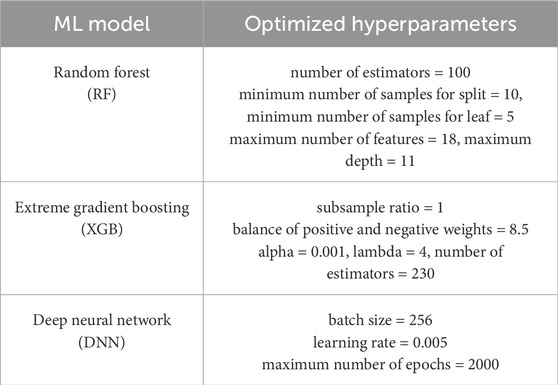
Table 1. Optimized hyperparameters for the ML models.

3.3 Extreme gradient boosting (XGB)

XGB is an advanced implementation of a gradient-boosting algorithm that aims to improve the performance and speed of traditional methods. It was designed to handle large datasets and has become popular in data science competitions. The XGB algorithm operates by building a series of decision trees and iteratively improving them by adjusting their weights based on errors made in the previous iteration. It uses regularization techniques to prevent overfitting and handles missing values in the data. XGB has many hyperparameters that can be tuned to achieve the best performance.

We used a gradient-boosted regression tree that calculates the gradient of the loss function and updates the model parameters in a step-by-step manner. Bagging was also used in XGB to improve the stability and accuracy of the model. In bagging, multiple models are trained on different subsets of training data, and their predictions are combined to obtain a final prediction. This reduces the impact of outliers and overfitting. XGB uses a variant of bagging called stochastic gradient boosting, in which each tree is trained on random subsets of data and features. This further reduces the correlation between trees and improves the generalization performance of the model. GridSearchCV and MultiOutputRegressor were used to tune the hyperparameters and build the model with XGBRegressor. The root mean squared error (RMSE) was used as the loss function. The optimized hyperparameters for the XGB model are listed in Table 1.

3.4 Deep neural network (DNN)

DNN is a neural network composed of several layers of fully connected nodes that perform complex computations. DNNs are trained using a process called backpropagation, in which the model learns to adjust the weights of the connections between nodes in response to the input data. The layers of a DNN typically include the input, hidden, and output layers, with each layer performing a specific data transformation. The depth and complexity of a DNN can be customized to the specific task at hand, with deeper networks typically able to learn more abstract features from the data. However, DNN training can be computationally expensive and requires a large amount of data to prevent overfitting.

Figure 1 show the architecture of the proposed DNN model. In the first group, four fully connected (FC) hidden layers were created to extract features from the input parameters. Increasing the number of units enabled the model to capture low-level features. Subsequently, the second group, consisting of three FC hidden layers, was created to encode high-level features by reducing the number of units. In all the hidden layers without an output layer, a rectified linear unit (ReLU) (Nair and Hinton, 2010) was applied as the activation function. After all activation functions, batch normalization (BN) was used to reduce the internal covariate shift and achieve a stable distribution during training (Ioffe and Szegedy, 2015). The weights were initialized using a Glorot uniform initializer (Glorot and Bengio, 2010) and the biases were set to zero before training. The Adam optimizer (Kingma and Ba, 2015) was used to adjust the weights of the FC hidden layers. The output layer was connected to the last hidden layer by applying a linear activation function. The loss of the DNN model was calculated using the MSE and mean absolute error (MAE). The optimized hyperparameters for the DNN model are summarized in Table 1.

Figure 1

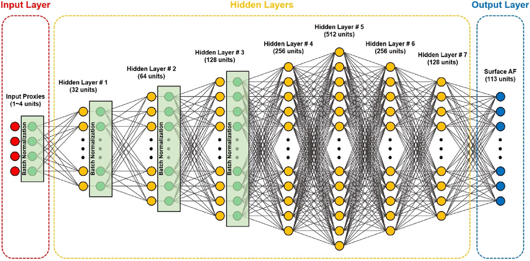
Figure 1. Architecture of DNN model.

4 ML model training

In this section, we present the input proxies and pairings used for training. We considered four SPs: H, T_G, V_S30, and V_S,soil (time-averaged V_S of the soil profile). As discussed in the previous section, VS30 is the most widely used SP in site amplification models. Its adoption was first popularized through foundational studies linking site classification to amplification (Borcherdt, 1994, Boore et al., 1997). Subsequent empirical GMMs (Choi and Stewart, 2005, Walling et al., 2008) further confirmed its utility, while more recent studies have refined its predictive capability and limitations (Seyhan and Stewart, 2014, Sandıkkaya and Dinsever, 2018, Harmon et al., 2019; Aaqib et al., 2021). Studies suggest that the amplification prediction can be improved by using T_G in addition to V_S30 (Harmon et al., 2019; Aaqib et al., 2021). H and V_S,Soil are the parameters used for site classification in the seismic design code of Korea (MOLIT, 2016). We used two MPs to represent the intensity and frequency characteristics of the input ground motions: PGA and S_S. S_S is defined as the averaged SA from 0.1 to 0.5 s, which is the range used to determine the short-period site amplification factor (F_a) in Korea (MOLIT, 2016). We used S_S because the short-period SA is estimated to have a significant influence on the amplification characteristics of shallow bedrock sites.

Table 2 summarizes the combinations used for the training. For Cases 1–4, only single SPs were used, whereas two pairs of SPs were used in Cases 5 and 6. Cases 1–6 were used to evaluate the performance of the SPs in predicting only linear amplification. For Case 7, one SP and one MP were used, respectively, which were V_S30 and PGA. Note that V_S30 and PGA were the inputs for the F_NL of the AEA21 model. Case 7 was only used to train the nonlinear amplification component for comparison with the AEA21 model’s F_NL. In Cases 8–11, two SPs and one MP were paired. Two SPs and two MPs were paired in Cases 12 and 13, respectively. Cases 8–13 were trained to predict both linear and nonlinear components.

Table 2

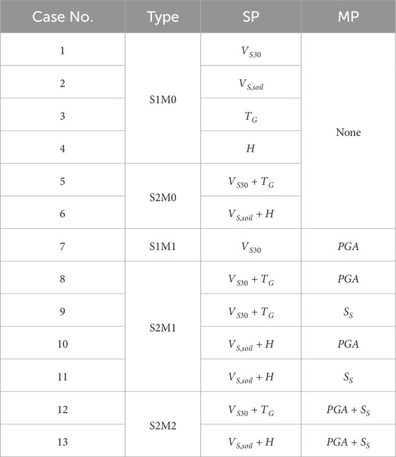
Table 2. Selected combinations using SPs and MPs.

To train the ML models, we randomly selected 80% of the linear and nonlinear SRA outputs as the training set and evaluated their performance using the remaining 20% as the test set. Additionally, we performed 5-fold cross-validation to check whether the trained models were overfitted. We compared the results between each fold and used the fold with the smallest loss because no significant differences were observed. The ML models were trained on a Windows-based operating system with a 64 GB NVIDIA RTX A6000 GPU and 32 GB of RAM.

5 Prediction of amplification using machine learning models

Linear and nonlinear amplifications were predicted using the proposed RF, XGB, and DNN models. The coefficient of determination (R²) and standard deviation (SD) were calculated to compare the results of the ML models. We show the sensitivity of the proxy pairing to the predictions, the results of which are presented in detail in the following section.

5.1 Effect of proxy pairing

In this section, the effect of the pairs of input proxies used to train the linear and nonlinear components of the amplification model on the performance of the ML model is presented. Only the results of the DNN model are presented to focus solely on the influence of the input proxies.

Figures 2, 3 compare the calculated and predicted linear amplification components of SA at T = 0.01 and 0.2 s, respectively, for all combinations of input proxies. For T = 0.01 s (Figure 2), Cases 1–3 had similar R² values to (F_LIN)_Vs30, but Case 4 had a lower R² value. For T = 0.2 s (Figure 3), Cases 1 and 3 produced slightly higher or similar R² values compared with (F_LIN)_Vs30, whereas Cases 2 and 4 had significantly lower R² values than (F_LIN)_Vs30. The comparisons confirmed that the two SPs used in the AEA21 model, V_S30 and T_G, are critical proxies that strongly correlate with linear amplification. This finding is supported by previous studies as well as the results of this study, where the combination of V_S30 and T_G led to improved prediction accuracy. The DNN model cannot significantly improve the prediction accuracy relative to the regression-based model for single-proxy cases. For direct comparisons of the performances of AEA21 and DNN models, predictions using the same inputs should be analyzed. Cases 1 and 5 produced 9.9% and 19.2% increases in R² compared with (F_LIN)_Vs30 and (F_LIN)_Vs30+TG, respectively. Thus, increments in prediction accuracy using the ML algorithm were not pronounced when applying identical inputs, although the degree of outperformance was higher for the two proxy cases.

Figure 2

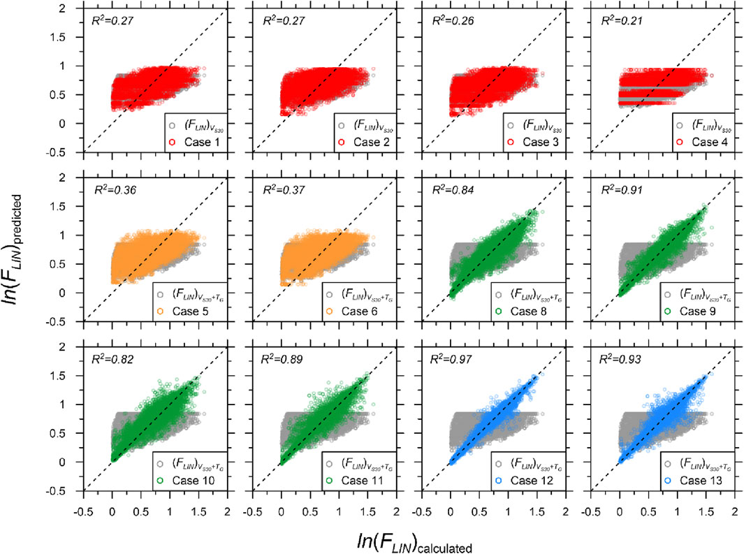
Figure 2. Comparison of calculated and predicted linear amplifications using AEA21 (gray) and DNN-based models at T = 0.01 s for selected pairings: S1M0 (red), S2M0 (orange), S2M1 (green), and S2M2 (blue). R² values of both (F_LIN)_VS30 and (F_LIN)_VS30+TG are 0.24.

Figure 3

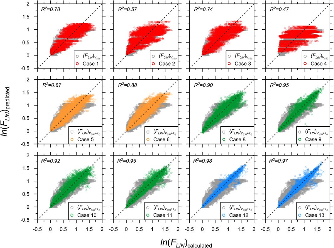
Figure 3. Comparison of calculated and predicted linear amplifications using AEA21 (gray) and DNN-based models at T = 0.2 s for selected pairings: S1M0 (red), S2M0 (orange), S2M1 (green), and S2M2 (blue). R² values of both (F_LIN)_VS30 and (F_LIN)_VS30+TG are 0.71 and 0.73, respectively.

The accuracy significantly improved relative to that of (F_LIN)_Vs30+TG when an MP was added (Cases 8–11). This improvement in accuracy completely contrasted the case in which an SP was added, which produced a marginal performance enhancement. S_S was observed to result in a higher prediction accuracy compared with PGA, most likely because it contained both intensity and frequency content information across a short period range, which is particularly relevant for the amplification of shallow bedrock sites. The use of two MPs along with two SPs resulted in a significantly higher accuracy. Although the differences between Cases 12 and 13 were marginal, the combination of V_S30 + T_G and the two MPs produced the most favorable predictions.

To further evaluate the influence of input proxy pairs on model performance, the R² values were visualized, as shown in Figure 4. The R² values for the AEA21 and LEA23 models alongside Cases 1 through 13 of the DNN-based models for F_LIN and F_NL. A clear improvement in model performance is observed as the number of proxies increase, particularly in Cases 8–13, where the addition of MPs led to consistently higher R² values. Notably, Case 12, which used V_S30 + T_G and two MPs, produced the highest R² values for both linear and nonlinear components. These results further support the conclusion that the DNN model benefits from well-paired proxy inputs.

Figure 4

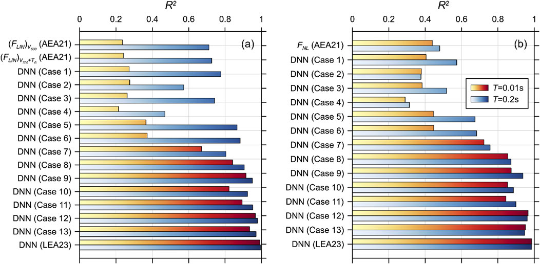
Figure 4. Comparison of R² for DNN-based models with AEA21 and LEA23 models across all proxy combinations at T = 0.01 and 0.2 s: (a) F_LIN, (b) F_NL.

Figure 5 shows the SDs of the residuals between the predicted and calculated amplifications plotted against V_S30. Among the single SP models, V_S30-based Case 1 produced the smallest SD for the entire V_S30 range, closely followed by T_G-based Case 3. H- and V_S,Soil-based models yielded significantly higher SDs. This was not surprising as they are designed to be used as pairs. Note that Cases 1 and 3 produced similar SDs compared to (F_LIN)_Vs30, indicating that ML is not much better than regression when using a single parameter.

Figure 5

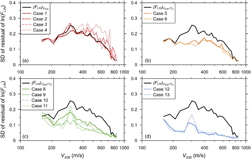
Figure 5. Comparison of SDs of residuals of F_LIN of simulated spectral accelerations at T = 0.2 s and predictions by DNN-based models for all pairings: (a) S1M0, (b) S2M0, (c) S2M1, (d) S2M2.

For Cases 5 and 6, the use of the two SPs noticeably decreased the SDs. An important characteristic of using the two SPs is their differences from the AEA21 model. The DNN model clearly improved the prediction compared with the regression-based model, indicating that the ML model becomes more effective when using multiple proxies. Similar to the R² comparisons, the use of MPs significantly improved the performance, yielding significant reductions in SDs. Overall, S_S was demonstrated to be more effective than PGA. The SD increased sharply near 300 m/s for Cases 8–11, which employed a single MP, except for Case 9, which used V_S30 + T_G as well as S_S. The large scatter near the resonance period of the stiff profiles was significantly reduced when trained with S_S.

Cases 12 and 13 revealed that the use of multiple MPs reduced the SDs in all periods. An abrupt spike in the SD near 300 m/s was again visible in both cases. Although using double MPs was not as effective for sites with V_S30 of approximately 300 m/s, the SDs were nevertheless lower compared with the single MP predictions. Case 12 exhibited the smallest SD among all the cases, highlighting that V_S30 + T_G paired with two MPs was the best combination among all the cases simulated in this study.

Figure 6 compares the predicted F_NL for T = 0.2 s calculated using the AEA21 and DNN models with the calculated amplifications. Case 7, which used identical inputs to F_NL, produced a 65% increase in R² compared with the AEA21 model. This was because F_NL only accounted for V_S30 indirectly. Using multiple SPs produced an excellent fit, particularly when paired with S_S, achieving an R² = 0.94. This demonstrated that S_S is a better proxy than PGA for estimating the nonlinear component, as was also demonstrated for the linear component. When both MPs were used for training, the predictions improved marginally. Comparisons of the nonlinear component predictions revealed that it is important to pair SPs with MPs. Note that the nonlinear component of the AEA21 model had a lower accuracy than the linear component. However, the accuracy of the nonlinear DNN model was similar to that of the linear model. Therefore, we strongly recommend that both SPs be included in the training of nonlinear components.

Figure 6

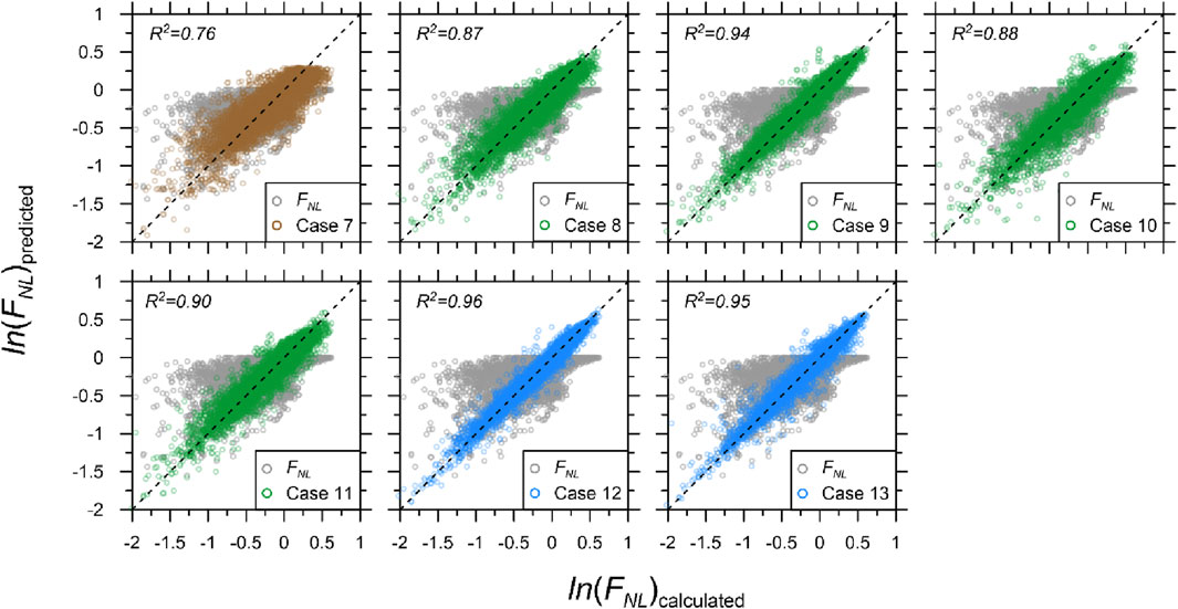
Figure 6. Comparison of calculated and predicted nonlinear amplifications using AEA21 (gray) and DNN-based models at T = 0.2 s for selected pairings: S1M1 (brown), S2M1 (green), and S2M2 (blue). R² of F_NL is 0.46.

Figure 7 plots the SDs of the residuals for comparison purposes. As expected, the SD decreased as the number of input parameters increased. Cases 9, 12, and 13 produced similar performances in terms of SD. The difference in the calculated SD between the DNN and regression models was significant, indicating that ML is considerably effective in reducing the scatter across the entire V_S30 range.

Figure 7

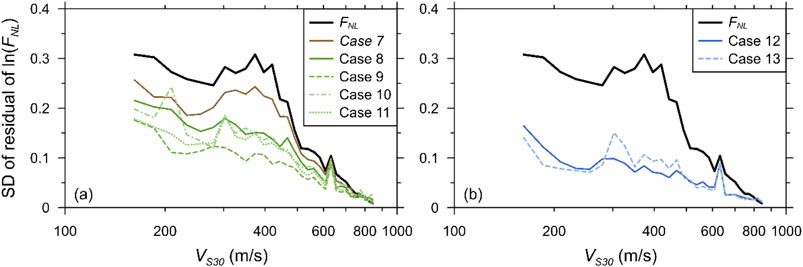
Figure 7. Comparison of SDs of residuals of F_NL of simulated spectral accelerations and predictions using DNN-based models for all combinations at T = 0.2 s: (a) S1M1 and S2M1, (b) S2M2.

5.2 Performance of ML algorithm

In this section, the performance of the 3 ML algorithms is evaluated. Only Cases 9 and 12, which produced more accurate predictions than other methods, were compared. Figure 8 compares the R² of 3 ML models for the two cases. The performance of the ML model was observed to depend on the parameters used for training. In Case 9 shown in Figure 8, the XGB model produced the best fit for the calculated outputs, followed by the DNN and RF models. The predictions of the XGB and DNN models were similar at periods shorter than 0.1 s, but the DNN model produced pronounced misfits from 1.0 to 2.0 s. For Case 12, the DNN model yielded the most agreeable predictions at all periods. Noticeable increases in the prediction accuracy at low periods were observed in the DNN model. Additionally, the bump from 1.0 to 2.0 s was removed.

Figure 8

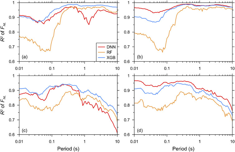
Figure 8. Comparison of R² of linear amplification component predicted using RF-based, XGB-based, and DNN-based models: (a) F_LIN of Case 9, (b) F_LIN of Case 12, (c) F_NL of Case 9, (d) F_NL of Case 12.

The SDs of the residuals for F_LIN and F_NL using the 3 ML models at four selected spectral periods (0.01, 0.1, 0.2, and 0.5 s) are plotted against V_S30 in Figures 9, 10, respectively. The performance of the ML models was revealed to depend on T. For T = 0.01 s, the DNN model produced the smallest SD for the wide range of V_S30 followed by the XGB and RF models. The differences between the models were clearly visible. For the DNN model, the SD of the residuals was not significantly affected by V_S30 except for a pronounced increase in the SD at the lowest V_S30 below 180 m/s. Both the XGB and RF models exhibited higher fluctuations with respect to V_S30. For longer periods, the XGB model displayed a performance similar to that of the DNN model. However, the RF model exhibited the highest SD, demonstrating the poorest performance.

Figure 9

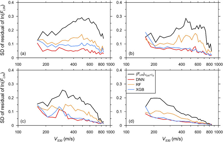
Figure 9. Comparison of SDs of residuals of F_LIN predicted by AEA21, DNN-based, RF-based, and XGB-based models against V_S30 for Case 12: (a) T = 0.01 s, (b) T = 0.1 s, (c) T = 0.2 s, (d) T = 0.5 s.

Figure 10

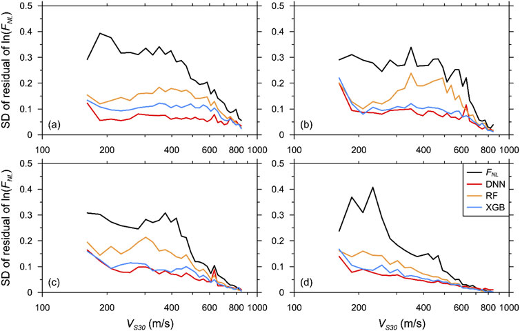
Figure 10. Comparison of SDs of residuals of F_NL predicted by AEA21, DNN-based, RF-based and XGB-based models against V_S30 for Case 12: (a) T = 0.01 s, (b) T = 0.1 s, (c) T = 0.2 s, (d) T = 0.5 s.

5.3 Effect of proxies in predicting site amplification

To enhance the interpretability of ML models, we analyzed feature importance using Shapley Additive Explanations (SHAP) and Partial Dependence (PD) methods. These methods are widely employed to explain how input features influence the predictions of complex, “black-box” models (Nandi and Das, 2025).

SHAP values quantify the contribution of each feature to the model’s prediction by considering the average marginal contribution of that feature across all possible combinations of features. Mathematically, the contribution of the ith proxy in terms of SHAP values is defined by Equation 3:

${\mathit{SHAP}}_{\mathit{i}}\left(\mathit{x}\right)={\displaystyle \sum _{\mathit{S}\subseteq \mathit{P}\{\left.\mathit{i}\right\}}}\frac{\left|\mathit{S}\right|!\left(\left|\mathit{P}\right|-\left|\mathit{S}\right|-1\right)!}{\left|\mathit{P}\right|!}\left[{\mathit{y}}_{\mathit{S}\cup \left\{\mathit{i}\right\}}\left({\mathit{x}}_{\mathit{S}\cup \left\{\mathit{i}\right\}}\right)-{\mathit{y}}_{\mathit{S}}\left({\mathit{x}}_{\mathit{S}}\right)\right](3)$

where P is the set of all proxies, S is a subset of proxies not containing ith proxy, and |P| and |S| are the number of proxies in P and S, respectively. f_x denotes the model prediction when only proxies in S are included. y_S∪{i} and y_S are model outputs with and without the ith proxy, respectively. This ensures that SHAP fairly distributes the prediction among features based on their cooperative contributions.

Partial dependence (PD) illustrates how the model’s prediction changes as a single proxy varies, while marginalizing over the other proxies. The PD function for jth proxy is given by Equation 4:

${PD}_j\left(x_j\right)=\frac{1}{n}{\displaystyle \sum _{i=1}^n}f\left(x_j,x_{i,-j}\right)(4)$

where x_i,−j represents all features except j, and n is the number of proxies. PD thus reflects the global trend of how a feature influences the predicted output, averaged across the data distribution.

Figure 11 shows the mean absolute SHAP values summed across 14 selected periods, reflecting the overall importance of each proxy. For F_LIN, V_S30 emerges as the most influential proxy, followed by T_G, PGA, and S_S. For F_NL, V_S30 remains dominant, though the contributions of T_G and S_S increase relative to F_LIN. Notably, T_G shows the largest proportional increase in influence, rising by a factor of approximately 1.7, followed by PGA and V_S30, which increase by factors of 1.5 and 1.3, respectively. These trends indicate that as nonlinearity becomes more pronounced, the predictive contributions of individual proxies also increase. Moreover, the heightened contribution of T_G may be attributed to period lengthening caused by modulus degradation effects, while the increased importance of PGA aligns with its established role as a key parameter in conventional nonlinear amplification models. This suggests that site stiffness, represented by V_S30, is consistently the most critical factor in site amplification, with T_G and S_S assuming more significant roles under nonlinear conditions. While motion intensity proxies are theoretically central to nonlinear response, our data-driven models capture the coupled nature of site and motion effects, leading to an observable importance of site proxies in predicting F_NL.

Figure 11

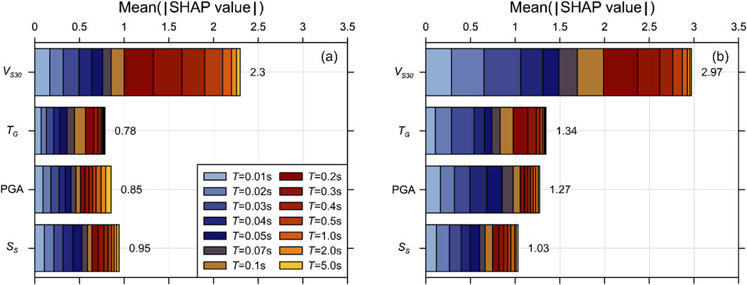
Figure 11. Proxy importance by SHAP values for Case 12 using XGB-based model: (a) F_LIN and (b) F_NL.

Figures 12, 13 present SHAP and PD analyses for Case 12 at T = 0.2 s, using the XGB-based model to predict F_LIN and F_NL, respectively. For F_LIN, the SHAP scatter plots show considerable variability, with V_S30 contributing strongly and positively up to approximately 400 m/s, beyond which its influence reverses. The PD curves reflect this trend, exhibiting patterns similar to upper-bound behavior for V_S30 and T_G. T_G demonstrates moderate positive influence, while PGA and S_S show relatively smaller contributions, suggesting limited sensitivity for F_LIN at this period. In the case of F_NL, V_S30 displays a clear transition from negative to positive contributions between approximately 200 and 500 m/s, indicating changes in nonlinear site behavior depending on soil stiffness. T_G again shows moderate positive influence, particularly at periods between 0.3 and 0.5 s, and exhibits patterns similar to lower-bound of the SHAP values. PGA and S_S contribute less significantly, with subtle effects captured in the PD curves. Notably, the magnitude of SHAP values for F_NL is overall higher than for F_LIN, indicating stronger nonlinear interactions. The flat or abrupt PD patterns for PGA and SS were found to coincide with sparsely populated regions in the dataset, particularly above 0.5 g and near 1.0 g, respectively. This sparsity affects the stability of the average marginal predictions in those regions. Although the PD curves may appear unexpectedly flat, this is consistent with model behavior trained on imbalanced feature distributions.

Figure 12

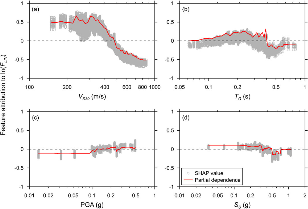
Figure 12. Feature attribution for predicting linear amplifications at T = 0.2 s for Case 12 using XGB-based model, for proxies: (a) V_S30, (b) T_G, (c) PGA, and (d) S_S.

Figure 13

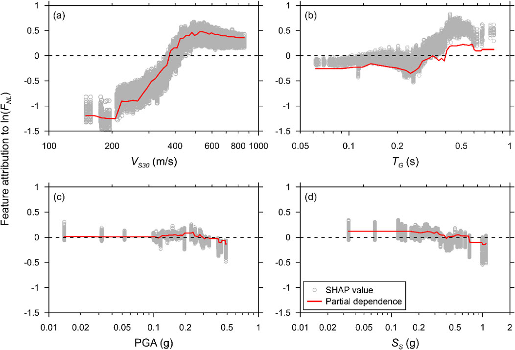
Figure 13. Feature attribution for predicting nonlinear amplifications at T = 0.2 s for Case 12 using XGB-based model, for proxies (a) V_S30, (b) T_G, (c) PGA, and (d) S_S.

SHAP and PD analyses confirm that V_S30 is the dominant predictor for both F_LIN and F_NL, while T_G provides meaningful additional predictive power. PGA and S_S contribute less prominently. These findings may also reflect limitations inherent in this study. Only a relatively small number of high-intensity ground motions were used, and the analysis focused solely on the perfectly correlated V_S profiles that increase with confining pressure. As a result, pronounced nonlinear soil behavior may not have fully manifested in the data. This limitation likely contributed to the relatively lower importance observed for PGA and S_S, compared to the SPs.

5.4 Comparison with the rigorous ML model

In this section, we compare the developed model with the rigorous LEA23 model. Figure 14 shows the R² and MSE of both F_LIN and F_NL as functions of the period. As expected, the array-input-based LEA23 model produced more accurate predictions than the proxy-based DNN model. For F_LIN, the LEA23 model produced an excellent fit with the simulation outputs, resulting in an R² higher than 0.96 in all periods. Case 12 model also produced excellent predictions, with an R² ranging from 0.93 to 0.99. Case nine model using only a single MP resulted in a relatively much lower R², but still yielded R² higher than 0.9 except at a low period range shorter than 0.1 s and around 1.0 s. Similar trends were observed when plotting the MSE of F_LIN.

Figure 14

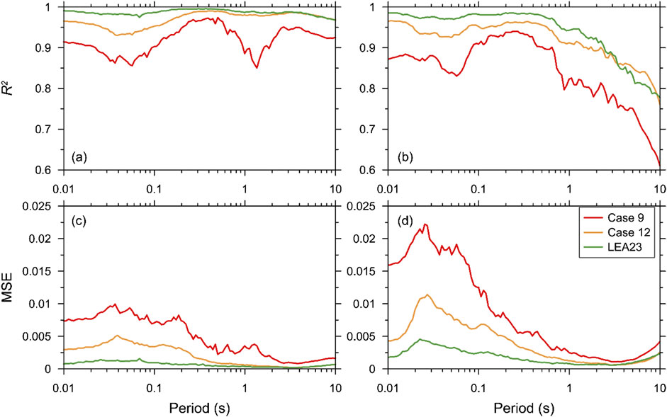
Figure 14. Comparison of R² and MSE of DNN-based and LEA23 models: (a) R² of F_LIN, (b) R² of F_NL, (c) MSE of F_LIN, (d) MSE of F_NL.

For F_NL, the LEA23 model again produced excellent predictions at T < 0.1 s, but rapidly decayed in R² at longer periods. This demonstrated that even the rigorous model is not as successful in predicting the nonlinear components over long periods and that additional training is required. Again, Case 12 produced a slightly lower R² but performed similarly over all periods. Case 9 performed poorly at all periods, falling below 0.8 at T > 1.0 s.

Figure 15 plots the SDs of residuals for F_LIN and F_NL using the LEA23 and DNN models at two selected spectral periods (0.01 and 0.2 s) against V_S30. The differences between the models were clearly visible. The rigorous model exhibited the lowest SD for all V_S30 compared with the DNN models. However, the DNN model using four proxies (Case 12) again produced stable SDs across all V_S30 except for a few scattered bumps when predicting both the linear and nonlinear components.

Figure 15

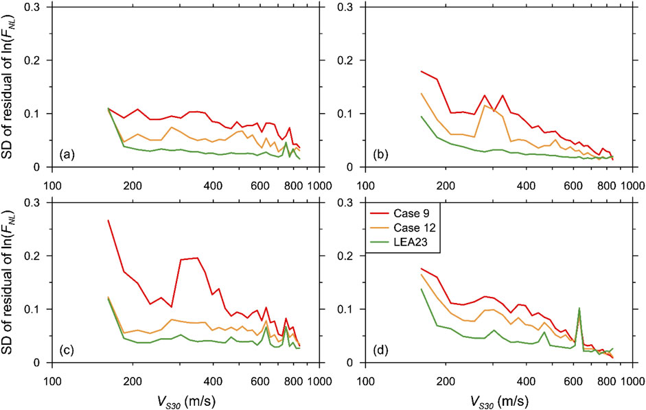
Figure 15. Comparison of SDs of residuals of both linear and nonlinear amplification components predicted using DNN-based and LEA23 models against V_S30 (Cases 9 and 12): (a) F_LIN at T = 0.01 s, (b) F_LIN at T = 0.2 s, (c) F_NL at T = 0.01 s, (d) F_NL at T = 0.2 s. Comparison of SD of the residuals of linear amplification component predicted using the AEA21, DNN-based, RF-based, and XGB-based models against V_S30 at T = 0.01, 0.1, 0.2, and 0.5 s (Case 12).

Surprisingly, despite the discrepancy in the training data, the differences in the performances of the four proxy and rigorous DNN models were not significant. The limited variability in the soil profiles of the shallow bedrock sites considered in this study probably resulted in the exceptional performance of the proxy-based ML model. Further studies are required to evaluate whether this trend is valid only for shallow bedrock sites with strong V_S reversals or applies to other types of sites.

To provide a comprehensive comparison, Table 3 summarizes the performance of the models developed in this study alongside existing models (AEA21 and the rigorous LEA23 model. Widely used performance metrics (R², MSE, RMSE, and MAE) as well as correlation coefficient (CC) were selected for this comparison. Among all models, the regression-based AEA21 model exhibited the lowest predictive performance across both F_LIN and F_NL, whereas the LEA23 model achieved the highest accuracy due to its detailed input features. Notably, our proxy-based model (Case 12), relying on only four proxies, demonstrated performance metrics comparable to the LEA23 model, underscoring the practicality and efficiency of the proposed approach. These findings confirm that proxy-based ML models can achieve predictive capabilities similar to more complex models, highlighting their potential for practical application in regional GMM and seismic hazard analysis.

Table 3

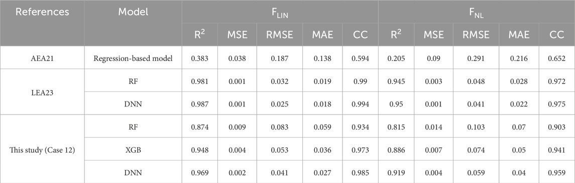
Table 3. Performance metrics of Case 12 compared to existing site amplification models.

6 Summary and conclusion

The objective of this study was to develop proxy-based linear and nonlinear site amplification models for shallow bedrock sites using ML for possible applications in a regional GMM. Four SPs were tested: H, T_G, V_S30, and V_S,Soil. We used two MPs to represent the intensity and frequency characteristics of the input ground motions: PGA and S_S. The outputs of the 1D linear and nonlinear SRAs performed for shallow bedrock sites with H < 30 m were used for the training. We explored the effects of SP and MP pairings on the performance of the ML models. We used 3 ML algorithms to evaluate the method that produced the most favorable predictions: RF, XGB, and DNN.

We compared the predictions of the ML models with those of the reference regression-based model proposed by Aaqib et al. (2021), referred to as the AEA21 model. Two linear models were proposed by Aaqib et al. (2021) One was conditioned only on V_S30, whereas the other was dependent on the two SPs (V_S30 and T_G). The nonlinear component depends on PGA and is indirectly conditioned on V_S30. For the linear component, the performance of the ML models did not improve significantly when using SPs. However, the prediction accuracy significantly improved when using MPs in addition to SPs for training the linear model. Using S_S yielded a greater improvement in the predictions because it contains information on both the intensity and frequency. The use of two SPs (V_S30 and T_G) and two MPs (PGA and S_S) produced excellent predictions of linear amplification.

Similar trends were observed for the nonlinear components. A case that used V_S30 and PGA, identical to the AEA21 model, produced a significant increase in prediction accuracy. This was because AEA21 accounts for V_S30 only indirectly. Using multiple SPs produced even better fits when paired with either S_S or MPs. Comparisons of the nonlinear component predictions revealed that both SPs should be considered in addition to MP. Note that the nonlinear component of the AEA21 model exhibited a lower accuracy than the linear component. However, the accuracy of the nonlinear DNN model was similar to that of the linear model. Therefore, we strongly recommend including SPs directly in the training of the nonlinear components.

The performance of the 3 ML algorithms considered in this study was tested by applying the recommended combination of SP and MP. The RF algorithm exhibited the poorest performance, displaying lower prediction accuracies across the entire range of analyses. The XGB model produced the best predictions for the linear component, whereas the DNN model outperformed the nonlinear component.

The proxy-based DNN model was also compared with the rigorous ML model of Lee et al. (2023), which was trained with larger input data, including the full V_S profile and input motion response spectrum. Although the proxy-based model was trained using only four parameters, it surprisingly produced agreeable predictions. This may have been because the constraint enforced on the site type, utilizing only profiles with bedrock less than 30 m without stiffness reversal, resulted in good prediction accuracy. Generalization of this feature should be applied with caution to other types of sites. Future studies should be conducted on various types of sites to investigate the capability of the proxy-based site amplification ML model.

To enhance interpretability and transparency of the ML models, this study employed SHAP and PD methods. These analyses confirmed that V_S30 remains the dominant predictor for both linear and nonlinear amplification components, highlighting the critical role of site stiffness in seismic response. T_G demonstrated meaningful contributions, especially under nonlinear conditions, likely related to period lengthening effects from modulus degradation. Although PGA and S_S had less influence overall, their importance increased under stronger nonlinear conditions, aligning with their roles in conventional amplification models. These analyses revealed the coupled behavior of SP and MP, providing essential insights into the model’s internal decision-making processes. While our findings are robust, they may be influenced by the limited number of high-intensity ground motions used and the specific V_S profiles examined, which may have reduced the manifestation of pronounced nonlinear soil behavior.

The findings of this study demonstrate that advanced ML models offer significant potential for improving the accuracy and adaptability of site amplification predictions at shallow bedrock sites. These improvements can play a critical role in seismic risk mapping, performance-based design, and urban land-use planning in earthquake-prone regions. By enabling more precise, site-specific hazard estimations, AI-integrated models support safer zoning decisions, targeted retrofitting of vulnerable structures, and the prioritization of critical infrastructure investments.

Looking forward, the application of emerging AI techniques, including transformers, physics-informed neural networks, and generative models, holds great promise for capturing the complex, nonlinear behaviors of seismic ground response and for integrating multi-source urban data into hazard assessments. We advocate for close interdisciplinary collaboration between geotechnical engineers, AI researchers, and urban planners to develop predictive models that are both technically robust and practically transformative, ultimately contributing to safer and more resilient urban environments.

Although this study does not explicitly address land subsidence, previous research indicates that subsidence can alter shear-wave velocity profiles and affect site amplification characteristics (Mayoral et al., 2017; Mayoral et al., 2019). These changes may shift the predominant period and modify the amplitude of seismic waves. Future studies should consider the influence of subsidence, particularly in regions experiencing significant ground deformation.

Data availability statement

The raw data supporting the conclusions of this article will be made available by the authors, without undue reservation.

Author contributions

Y-GL: Data curation, Methodology, Writing – review and editing, Conceptualization, Validation, Supervision, Software, Formal Analysis, Writing – original draft, Visualization. DP: Conceptualization, Supervision, Writing – review and editing. O-SK: Writing – review and editing, Supervision, Conceptualization.

Funding

The author(s) declare that financial support was received for the research and/or publication of this article. This work was supported by the National Research Foundation of Korea (NRF) grant funded by the Korean Government (MSIT) (NRF-2022R1A2C3003245).

Conflict of interest

The authors declare that the research was conducted in the absence of any commercial or financial relationships that could be construed as a potential conflict of interest.

Generative AI statement

The author(s) declare that no Generative AI was used in the creation of this manuscript.

Publisher’s note

All claims expressed in this article are solely those of the authors and do not necessarily represent those of their affiliated organizations, or those of the publisher, the editors and the reviewers. Any product that may be evaluated in this article, or claim that may be made by its manufacturer, is not guaranteed or endorsed by the publisher.

References

Aaqib, M., Park, D., Adeel, M. B., Hashash, Y. M. A., and Ilhan, O. (2021). Simulation-based site amplification model for shallow bedrock sites in Korea. Earthq. Spectra 37 (3), 1900–1930. doi:10.1177/8755293020981984

CrossRef Full Text | Google Scholar

Agata, R., Shiraishi, K., and Fujie, G. (2025). Physics-informed deep learning quantifies propagated uncertainty in seismic structure and hypocenter determination. Sci. Rep. 15 (1), 1846. doi:10.1038/s41598-024-84995-9

PubMed Abstract | CrossRef Full Text | Google Scholar

Assimaki, D., Li, W., Steidl, J. H., and Tsuda, K. (2008). Site amplification and attenuation via downhole array seismogram inversion: a comparative study of the 2003 miyagi-oki aftershock sequence. Bull. Seismol. Soc. Am. 98 (1), 301–330. doi:10.1785/0120070030

CrossRef Full Text | Google Scholar

Bergamo, P., Hammer, C., and Fäh, D. (2021). On the relation between empirical amplification and proxies measured at Swiss and Japanese stations: systematic regression analysis and neural network prediction of amplification. Bull. Seismol. Soc. Am. 111 (1), 101–120. doi:10.1785/0120200228

CrossRef Full Text | Google Scholar

Boore, D. M., Joyner, W. B., and Fumal, T. E. (1997). Equations for estimating horizontal response spectra and peak acceleration from Western North American earthquakes: a summary of recent work. Seismol. Res. Lett. 68 (1), 128–153. doi:10.1785/gssrl.68.1.128

CrossRef Full Text | Google Scholar

Borcherdt, R. D. (1994). Estimates of site-dependent response spectra for design (methodology and justification). Earthq. Spectra 10 (4), 617–653. doi:10.1193/1.1585791

CrossRef Full Text | Google Scholar

Castellaro, S., Mulargia, F., and Rossi, P. L. (2008). VS30: proxy for seismic amplification? Seismol. Res. Lett. 79 (4), 540–543. doi:10.1785/gssrl.79.4.540

CrossRef Full Text | Google Scholar

Cheng, K., and Ziotopoulou, K. (2023). Machine learning applications in geotechnical earthquake engineering: progress, gaps, and opportunities. Geo-Congress 2023, 493–505. doi:10.1061/9780784484692.050

CrossRef Full Text | Google Scholar

Chiou, B.-J., and Youngs, R. R. (2008). An NGA model for the average horizontal component of peak ground motion and response spectra. Earthq. Spectra 24 (1), 173–215. doi:10.1193/1.2894832

CrossRef Full Text | Google Scholar

Chiou, B.S.-J., and Youngs, R. R. (2014). Update of the chiou and youngs NGA model for the average horizontal component of peak ground motion and response spectra. Earthq. Spectra 30 (3), 1117–1153. doi:10.1193/072813EQS219M

CrossRef Full Text | Google Scholar

Choi, Y., and Stewart, J. P. (2005). Nonlinear site amplification as function of 30 m shear wave velocity. Earthq. Spectra 21 (1), 1–30. doi:10.1193/1.1856535

CrossRef Full Text | Google Scholar

Darendeli, M. (2001). “Development of a new family of normalized modulus reduction and material damping curves,” in Ph. D. Dissertation. Austin: University of Texas.

Google Scholar

Deepsoil, M. (2024). “A nonlinear and equivalent linear seismic site response of 1-D soil columns, user manual,” in V7.0. board of trustees of university of Illinois at urbana-champaign. Urbana, IL.

Google Scholar

Derras, B., Bard, P.-Y., and Cotton, F. (2017). VS30, slope, H800 and f0: performance of various site-condition proxies in reducing ground-motion aleatory variability and predicting nonlinear site response. Earth, Planets Space 69 (1), 133–21. doi:10.1186/s40623-017-0718-z

CrossRef Full Text | Google Scholar

Derras, B., Bard, P.-Y., Régnier, J., and Cadet, H. (2020). Non-linear modulation of site response: sensitivity to various surface ground-motion intensity measures and site-condition proxies using a neural network approach. Eng. Geol. 269, 105500. doi:10.1016/j.enggeo.2020.105500

CrossRef Full Text | Google Scholar

Glorot, X., and Bengio, Y. (2010). “Understanding the difficulty of training deep feedforward neural networks,” in Proceedings of the thirteenth international conference on artificial intelligence and statistics, 249–256.

Google Scholar

Groholski, D. R., Hashash, Y. M., Kim, B., Musgrove, M., Harmon, J., and Stewart, J. P. (2016). Simplified model for small-strain nonlinearity and strength in 1D seismic site response analysis. J. Geotech. GeoEnviron. Eng. 142 (9), 04016042. doi:10.1061/(ASCE)GT.1943-5606.0001496

CrossRef Full Text | Google Scholar

Harmon, J., Hashash, Y. M., Stewart, J. P., Rathje, E. M., Campbell, K. W., Silva, W. J., et al. (2019). Site amplification functions for central and eastern north america–part II: modular simulation-based models. Earthq. Spectra 35 (2), 815–847. doi:10.1193/091117EQS179M

CrossRef Full Text | Google Scholar

Hashash, Y. M., Ilhan, O., Uysal, H., Stewart, J. P., Nikolaou, S., Rathje, E. M., et al. (2021). Application of empirical and simulation-based site amplification models for central and eastern North America to selected sites. Earthq. Spectra 37, 1516–1533. doi:10.1177/87552930211020770

CrossRef Full Text | Google Scholar

Héloïse, C., Bard, P.-Y., Duval, A.-M., and Bertrand, E. (2012). Site effect assessment using KiK-net data: part 2—site amplification prediction equation based on f 0 and vsz. Bull. Earthq. Eng. 10, 451–489. doi:10.1007/s10518-011-9298-7

CrossRef Full Text | Google Scholar

Ilhan, O., Harmon, J. A., Numanoglu, O. A., and Hashash, Y. M. (2019). Deep learning-based site amplification models for central and eastern North America. London: CRC Press, 2980–2987.

Google Scholar

Ioffe, S., and Szegedy, C. (2015). Batch normalization: accelerating deep network training by reducing internal covariate shift International conference on machine learning, 448–456.

Google Scholar

Kim, S., Hwang, Y., Seo, H., and Kim, B. (2020). Ground motion amplification models for Japan using machine learning techniques. Soil Dyn. Earth. Eng. 132, 106095. doi:10.1016/j.soildyn.2020.106095

CrossRef Full Text | Google Scholar

Kingma, D. P., and Ba, J. (2015). “Adam: a method for stochastic optimization,” in 3rd international conference on learning representations, ICLR, 2015. San Diego, CA, USA.

Google Scholar

Kokusho, T., and Sato, K. (2008). Surface-to-base amplification evaluated from KiK-net vertical array strong motion records. Soil Dyn. earth. Eng. 28 (9), 707–716. doi:10.1016/j.soildyn.2007.10.016

CrossRef Full Text | Google Scholar

Lee, V. W., and Trifunac, M. D. (2010). Should average shear-wave velocity in the top 30 m of soil be used to describe seismic amplification? Soil Dyn. earth. Eng. 30 (11), 1250–1258. doi:10.1016/j.soildyn.2010.05.007

CrossRef Full Text | Google Scholar

Lee, Y.-G., Kim, S.-J., Achmet, Z., Kwon, O.-S., Park, D., and Di Sarno, L. (2023). Site amplification prediction model of shallow bedrock sites based on machine learning models. Soil Dyn. earth. Eng. 166, 107772. doi:10.1016/j.soildyn.2023.107772

CrossRef Full Text | Google Scholar

Ma, L., Han, L., and Feng, Q. (2024). Deep learning for high-resolution seismic imaging. Sci. Rep. 14 (1), 10319. doi:10.1038/s41598-024-61251-8

PubMed Abstract | CrossRef Full Text | Google Scholar

Mayoral, J., Tepalcapa, S., Roman-de La Sancha, A., El Mohtar, C., and Rivas, R. (2019). Ground subsidence and its implication on building seismic performance. Soil Dyn. Earth. Eng. 126, 105766. doi:10.1016/j.soildyn.2019.105766

CrossRef Full Text | Google Scholar

Mayoral, J. M., Castañon, E., and Albarran, J. (2017). Regional subsidence effects on seismic soil-structure interaction in soft clay. Soil Dyn. Earth. Eng. 103, 123–140. doi:10.1016/j.soildyn.2017.09.014

CrossRef Full Text | Google Scholar

MOLIT (2016). Korean building code 2016. Ministry Land, Infrastructure, Transp. South Korea.

Google Scholar

Mousavi, S. M., and Beroza, G. C. (2023). Machine learning in earthquake seismology. Annu. Rev. Earth Planet. Sci. 51 (1), 105–129. doi:10.1146/annurev-earth-071822-100323

CrossRef Full Text | Google Scholar

Mousavi, S. M., Ellsworth, W. L., Zhu, W., Chuang, L. Y., and Beroza, G. C. (2020). Earthquake Transformer—An attentive deep-learning model for simultaneous earthquake detection and phase picking. Nat. Commun. 11 (1), 3952. doi:10.1038/s41467-020-17591-w

PubMed Abstract | CrossRef Full Text | Google Scholar

Mousavi, S. M., Beroza, G. C., Mukerji, T., and Rasht-Behesht, M. (2024). Applications of deep neural networks in exploration seismology: a technical survey. Geophysics 89 (1), WA95–WA115. doi:10.1190/geo2023-0063.1

CrossRef Full Text | Google Scholar

Mucciarelli, M., and Gallipoli, M. R. (2006). “Comparison between VS30 and other estimates of site amplification in Italy,” in First European conference on earthquake engineering and seismology. Geneva, Switzerland.

Google Scholar

Nair, V., and Hinton, G. E. (2010). “Rectified linear units improve restricted boltzmann machines,” in 27th international conference on machine learning, Haifa, Israel.

Google Scholar

Nandi, B., and Das, S. (2025). Predicting max scour depths near two-pier groups using ensemble machine-learning models and visualizing feature importance with partial dependence plots and SHAP. J. Comput. Civ. Eng. 39 (2), 04025007. doi:10.1061/jccee5.cpeng-6150

CrossRef Full Text | Google Scholar

Pedregosa, F., Varoquaux, G., Gramfort, A., Michel, V., Thirion, B., Grisel, O., et al. (2011). Scikit-learn: machine learning in python. J. Mach. Learn. Res. 12, 2825–2830.

Google Scholar

Sandıkkaya, M. A., and Dinsever, L. D. (2018). A site amplification model for crustal earthquakes. Geosciences 8 (7), 264. doi:10.3390/geosciences8070264

CrossRef Full Text | Google Scholar

Seyhan, E., and Stewart, J. P. (2014). Semi-empirical nonlinear site amplification from NGA-West2 data and simulations. Earthq. Spectra 30 (3), 1241–1256. doi:10.1193/063013eqs181m

CrossRef Full Text | Google Scholar

Stambouli, A. B., Zendagui, D., Bard, P.-Y., and Derras, B. (2017). Deriving amplification factors from simple site parameters using generalized regression neural networks: implications for relevant site proxies. Earth, Planets Space 69 (1), 1–26. doi:10.1186/s40623-017-0686-3

CrossRef Full Text | Google Scholar

Toro, G. (1995). Probabilistic models of site velocity profiles for generic and site-specific ground-motion amplification studies.

Google Scholar

Walling, M., Silva, W., and Abrahamson, N. (2008). Nonlinear site amplification factors for constraining the NGA models. Earthq. Spectra 24 (1), 243–255. doi:10.1193/1.2934350

CrossRef Full Text | Google Scholar

Wang, X., Wang, Z., Wang, J., Miao, P., Dang, H., and Li, Z. (2023). Machine learning based ground motion site amplification prediction. Front. Earth Sci. 11, 1053085. doi:10.3389/feart.2023.1053085

CrossRef Full Text | Google Scholar

Zhang, X., and Zhang, M. (2024). Universal neural networks for real-time earthquake early warning trained with generalized earthquakes. Commun. Earth & Environ. 5 (1), 528. doi:10.1038/s43247-024-01718-8

PubMed Abstract | CrossRef Full Text | Google Scholar