Operation optimization of water-cooled central chilling system in a commercial office building based on the gray wolf optimization algorithm

In this study, the gray wolf algorithm was applied to optimize the water-cooled central chilling system operation in a commercial office building. The optimization objective was to maximize the system’s energy efficiency ratio by seeking the optimal number and load distribution of activated chillers, the number and approximate degree of activated cooling towers, and the number and frequency of activated chilled water pumps and activated cooling water pumps. The results show that by using the grey wolf optimization algorithm, the energy efficiency ratio of the refrigeration plant room in the design day increased from 5.03 to 5.51, yielding an increase of 9.67%. The annual comprehensive energy efficiency ratio increased from 5.50 to 6.15, or 11.82%.

1 Introduction

The energy consumption of buildings occupies approximately 70% of a city’s primary energy (Chen et al., 2019). It is crucial to improve building-energy efficiency for socially sustainable development (Hong et al., 2020). Central air conditioning systems consume more than two-thirds of a building’s total energy consumption (Ali et al., 2013). Thus, it is essential to improve the energy efficiency of central air conditioning systems to conserve building energy. Central chilling systems yield over 50% of total central air conditioning systems’ energy consumption (Luis et al., 2008). Therefore, the optimization of central chilling operations is key to central air conditioning system energy conservation.

Numerous recent studies have been conducted on the operational optimization of water-cooled central chilling systems (Jia et al., 2021). The control strategy of this subsystem and its disadvantages are summarized in Table 1. Sen Huang optimized both load distribution and operating chiller numbers based on chiller sequencing control (Huang et al., 2016). Sequencing control did not fully consider the performance differences of each chiller, making it impossible to optimize the load distribution and operating chiller numbers, thus preventing the optimal efficiency of energy systems. The operational parameter optimization of chiller plants has been conducted by particle swarm optimization (Karami and Wang, 2018; Chan et al., 2022; Deng et al., 2022; Gao et al., 2022). However, particle swarm optimization has several disadvantages, such as premature convergence to a local rather than global optimum, parameter sensitivity, and restricted performance in constrained optimization problems. Chaoqun Zhuang proposed a risk-based robust optimal chiller sequencing control strategy to improve chiller operational energy efficiency and robustness (Zhuang et al., 2020). This approach also has several disadvantages and challenges, such as high computational complexity, model dependency, and conservatism. Chen et al. (2020) compared three sequencing control strategies, with their results indicating that the hourly control of chiller plants is optimal. Liu et al. (2023) studied the time limit of optimal calculation and the output of the optimal control strategy, with the result indicating that it not only has good optimization effect but also that confidence is increased considerably. Hu et al. (2024) recommended an improved flower pollination algorithm to optimize multi-chiller loading for higher robustness with a slightly reduced convergence rate. However, this also has several disadvantages and limitations, such as being prone to local optima, slow convergence in later stages, and insufficient accuracy.

Table 1

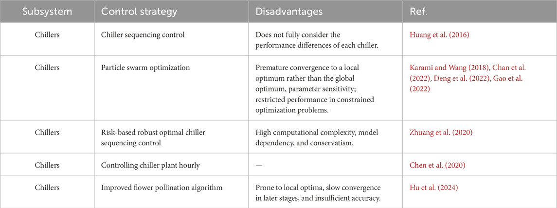
Table 1. Water-cooled central chilling system control strategy and its disadvantages.

The above research mainly focused on the optimization of chillers. Water-cooled central chilling systems consist of chillers, chilled water pumps, cooling water pumps, and cooling towers, which interact and influence each other. Therefore, although chillers consume a considerable amount of energy, the goal of water-cooled central chilling system optimization is not to minimize the energy consumption of chillers or any other individual device but to minimize the total power consumption of the system. Thus, this study aims to minimize the total power consumption of a water-cooled central chilling system.

Among emerging swarm intelligent algorithms, the gray wolf algorithm has the advantages of fewer set parameters, better robustness, and higher convergence speed and accuracy than with the swarm and genetic algorithms (Mirjalili et al., 2014). The gray wolf optimization algorithm has been applied in fields such as power (Harish Kumar and Mageshvaran, 2022) and medicine (Rajakumar et al., 2023). It is supposed to optimize the operation of water-cooled central chilling systems to improve their energy efficiency utilization. In this study, the gray wolf algorithm is implemented on a water-cooled central chilling system to improve its energy efficiency so as to provide a new efficient algorithm for water-cooled central chilling system energy conservation.

2 Central chilling system and its energy consumption model

2.1 Central chilling system description

This project investigated a commercial office building in Guangzhou with a construction area of approximately 12,000 m². The building’s main function is office space, with some commercial supporting functions. As depicted in Figure 1, the water-cooled central chilling system of this building consists of three chillers, three chilled water pumps, three cooling water pumps, and three cooling towers. The main parameters of the equipment are shown in Table 2. The operating parameters of its equipment, such as inlet and outlet water temperature, water flow, heat flux, operating frequency, and output power, are collected and monitored by a data monitoring platform.

Figure 1

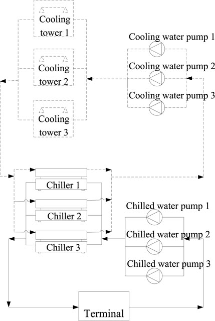
Figure 1. Water-cooled central chilling system.

Table 2

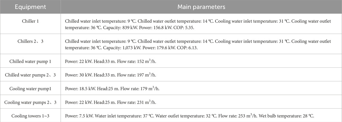
Table 2. Main parameters of equipment.

2.2 Water-cooled central chilling system energy consumption model

The energy consumption model of water-cooled chillers includes Gordon-NG (Gordon and NG, 1995), a Lee model (Lee and Lu, 2010), BQ model (Yik and Lam, 1998), and an MP model (Reddy and Andersen, 2002). An MP model is employed in this paper. Based on the sample parameters provided by the chiller manufacturer, the water-cooled chiller energy consumption model was obtained as Equation 1 by using the MATLAB multiple linear regression tool.

$\begin{array}{l}{W}_{ch}=W_{chr}\times f\left(PLR\right)\times f\left(T_{eo},T_{ci}\right)\\ =W_{chr}\times \left(a_1+a_{2}PLR+a_{3}PL{R}^2\right)\\ \times \left(a_4+a_5{T}_{eo}+a_6{T}_{eo}^2+a_7{T}_{ci}+a_8{T}_{ci}^2+a_9{T}_{eo}{T}_{ci}\right)\end{array}(1)$

where W_chr is the rated energy consumption of the chiller, PLR is the part-load ratio of the chiller, T_eo is the chilled water outlet temperature, T_ci is the cooling water inlet temperature, and a₀∼a₉ are regression coefficients.

Based on the actual operating data of the variable frequency water pump, it was found that the energy consumption and flow rate of the variable frequency water pump are in a quadratic polynomial relationship (Luan et al., 2008). Thus, based on the sample parameters provided by the water pump manufacturer, the chilled or cooling water pump energy consumption model was obtained as Equation 2 by a MATLAB multiple linear regression tool:

$W_p=b_0+b_{1}Q+b_2{Q}^2(2)$

where Q is the water pump flow rate, and b₀∼b₂ are the regression coefficients.

The Braun model is a semi-empirical model used for cooling tower performance; it can predict the heat dissipation and performance of cooling towers by combining thermodynamic equilibrium and empirical parameters (China Electronic Energy Conservation Technology Association, 2024). Thus, based on the sample parameters provided by the cooling tower manufacturer, the cooling tower’s fan energy consumption was calculated by Equations 3, 4.

$P_{fan}=\left(P_{fan,design}\right)\left(Fa{n}_{PLR}\right){\left(FRair\right)}^3(3)$

$m_a=Q_{tower}/{\epsilon }_a\left(h_{a,w,i-}{h}_{a,w,o}\right)(4)$

where P_{fan, design} is fan-rated energy consumption, Fan_PLR is the partial air volume power correction factor, FR_air is the ratio of the air volume to the rated air volume, m_a is the cooling tower’s air volume, Q_tower is the cooling tower’s heat dissipation, ε_a is air-side heat transfer efficiency, h_a,w,i is the cooling tower’s inlet air enthalpy, and h_a,w,o is the cooling tower’s outlet air enthalpy.

3 Optimization objective, variables, and control constraints

For the existing building’s water-cooled central chilling system, the objective was to obtain its optimal energy efficiency so as to maximize the energy efficiency ratio of the system.

The “energy efficiency ratio” is defined as the ratio of a water-cooled central cooling system’s total cooling capacity and its energy consumption. It can be calculated by Equation 5.

$EER=\frac{Q_{c,total}}{W_{ch}+W_p+P_{fan}}(5)$

where Q_c,total is the central cooling system’s total cooling capacity, and W_ch、W_p、and P_fan are the energy consumption of the chillers, water pumps, and cooling towers, respectively.

Thus, the optimization objective is described as the following Equation 6.

$\max EER=\max \left(\frac{Q_{c,total}}{W_{ch}+W_p+P_{fan}}\right)(6)$

The optimization variables of this project include the on/off status and operating parameters of each piece of equipment. For the chillers, these variables include number and load distribution of the activated chillers. For the cooling towers, the optimization variables include the approximation degree and the number of activated cooling towers. For the chilled and cooling water pumps, the optimization variables include the number and the frequency of the activated water pumps. The optimization variables are thus divided into two categories: continuous variables and discrete variables. Discrete variables include the on/off status of the chillers, water pumps, and cooling towers, where 0 and 1 represent the off and on status of the equipment, respectively. Continuous variables include the load distribution of the chillers, the frequency of the water pumps, and approximation degree of the cooling towers.

The optimization variables should comply with multiple physical and operational constraints, where the on/off status and operating parameters of each piece of equipment should meet its designed capability scope and practical operational requirements. The constraint conditions are described as the following Equation 7.

$\left\{\begin{array}{l}{T}_{approach,\min }<\Delta T_{approach}\\ f_{ct,\min }<f_{ct}<f_{ct,\max }\\ f_{chiller,\min }<f_{chiller}<f_{chiller,\max }\\ f_{chw\_pump,\min }<f_{chw\_pump}<f_{chw\_pump,\max }\\ f_{cw\_pump,\min }<f_{cw\_pump}<f_{cw\_pump,\max }\\ 0\le N_{ct}\le N_{ct,\max },N_{ct}\in \mathrm{{\rm Z}}\\ 0\le N_{chiller}\le N_{chiller,\max },N_{chiller}\in \mathrm{{\rm Z}}\\ 0\le N_{chw\_pump}\le N_{cw\_pump,\max },N_{chw\_pump}\in \mathrm{{\rm Z}}\\ 0\le N_{cw\_pump}\le N_{cw\_pump,\max },N_{cw\_pump}\in \mathrm{{\rm Z}}\end{array}\right.(7)$

where $∆{\mathrm{T}}_{\text{approac}\mathrm{h}}$ is the approximation degree of a cooling tower, ${\mathrm{f}}_{\text{ct}}$ is the flow rate distribution of the cooling tower, ${\mathrm{f}}_{\text{ciller}}$ is the load distribution of the chillers, ${\mathrm{f}}_{\text{chw}\_\text{pump}}$ is the chilled water pump frequency, and ${\mathrm{f}}_{\text{cw}\_\text{pump}}$ is the cooling water pump frequency. ${\mathrm{N}}_{\text{ct}}$, ${\mathrm{N}}_{\text{chiller}}$, ${\mathrm{N}}_{\text{chw}\_\text{pump}}$, and ${\mathrm{N}}_{\text{cw}\_\text{pump}}$ are the activated unit number of the cooling tower, chiller, chilled water pump, and cooling water pump, respectively. Z is a set of integers.

4 Algorithm design and application

4.1 Gray wolf optimization algorithm and mathematical models

The gray wolf optimization algorithm (GWO) simulates the behavior of gray wolves hunting prey (Mirjalili et al., 2014). As a social animal, they have a very obvious pyramid-like hierarchical system. Wolf α occupies the highest position and is responsible for decision-making and dominating the entire pack. Wolf β is located at the second highest level of the pyramid and is responsible for assisting the lead wolf αand conveying its instructions to subordinates. Wolf δ is located on the third level of the pyramid and is mainly responsible for reconnaissance, surveillance, hunting, and guarding the wolf pack. The bottom wolf layer accounts for the largest proportion of the gray wolf population and is responsible for hunting prey.

4.1.1 Encircling prey

Grey wolves encircle prey during the hunt. The mathematically model of encircling behavior is described as the following Equations 8, 9.

$\vec{D}=\left|\vec{C}·{\vec{X}}_p\left(t\right)-\vec{X}\left(t\right)\right|(8)$

$\vec{X}\left(t+1\right)={\vec{X}}_p\left(t\right)-\vec{A}·\vec{D}(9)$

where t indicates current iteration, $\vec{A}$ and $\vec{C}$ are coefficient vectors, ${\vec{X}}_p$ is the position vector of the prey, and $\vec{X}$ indicates the position vector of a gray wolf.

$\vec{A}$ and $\vec{C}$ are calculated by Equations 10, 11:

$\vec{A}=2\vec{a}·{\vec{r}}_1-\vec{a}(10)$

$\vec{C}=2·{\vec{r}}_2(11)$

where components of $\vec{a}$ are linearly decreased from 2 to 0 over the course of iterations, and ${\vec{r}}_1$ and ${\vec{r}}_2$ are random vectors in [0,1].

4.1.2 Hunting

It is supposed that α, β, and δ have better knowledge about the potential location of prey. Thus, we save the first three best solutions obtained so far and oblige the other search agents to update their positions according to Equations 12–14 according to the position of the best search agent.

$\vec{X}\left(t+1\right)=\frac{{\vec{X}}_1+{\vec{X}}_2+{\vec{X}}_3}{3}(12)$

${\vec{X}}_1={\vec{X}}_{\alpha }-{\vec{A}}_1·\left({\vec{D}}_{\alpha }\right),{\vec{X}}_2={\vec{X}}_{\beta }-{\vec{A}}_2·\left({\vec{D}}_{\beta }\right),{\vec{X}}_3={\vec{X}}_{\delta }-{\vec{A}}_3·\left({\vec{D}}_{\delta }\right)(13)$

${\vec{D}}_{\alpha }=\left|{\vec{C}}_1·{\vec{X}}_{\alpha }-\vec{X}\right|,{\vec{D}}_{\beta }=\left|{\vec{C}}_2·{\vec{X}}_{\beta }-\vec{X}\right|,{\vec{D}}_{\delta }=\left|{\vec{C}}_3·{\vec{X}}_{\delta }-\vec{X}\right|(14)$

As depicted in Figure 2, the gray wolf optimization algorithm is implemented as follows. First, the gray wolf population is initialized by generating n individuals and setting the initial values of a, A, and C. Next, the fitness of each individual is calculated, and the position of the lead wolves (X_α, X_β, and X_δ) are initialized. The algorithm then compares each individual’s fitness with that of X_α, X_β, and X_δ to determine the current optimal (X_α), second-best (X_β), and third-best (X_δ) solutions. Subsequently, the values of a, A, and C are recalculated, and each individual’s position is updated. The process repeats from the fitness evaluation step until the maximum iteration count is reached, at which point the algorithm terminates.

Figure 2

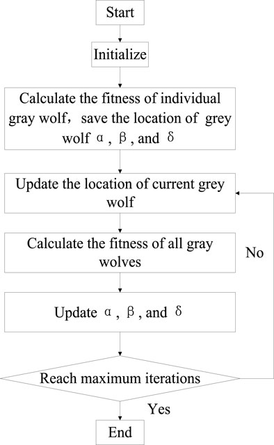
Figure 2. Gray wolf optimization algorithm flow chart.

4.2 GWO application

As for the load distribution of chillers, initialization generates a random value based on the minimum and maximum load limits of each chiller. If the initial total load is not zero, we adjust its load to the total cooling load through scaling. For the approximation degree of the cooling tower, initialization is implemented by randomly generating initial values between the minimum approximation degree and the maximum value 8 °C. Table 3 presents the detailed parameter boundary of each unit.

Table 3

Table 3. Parameter boundary of each unit.

If the solution violates these constraints during the update process, the following methods can be used to handle this problem. If the chiller load solution is lower than its minimum value or exceeds its maximum capacity, it will be brought back within the feasible range through a proportional adjustment function. In the process of updating the solution, if the approximation degree of the cooling tower exceeds its range, the program will truncate it within the feasible range by an adjustment function.

During the optimization process, discrete variables are adjusted by checking the values of continuous variables. Discrete variables are handled using the “threshold truncation” strategy. When the discrete variable approaches zero, the device shuts down; when the discrete variable exceeds a certain threshold, the device is turned on. If non-integer situations occur during the update process, the discrete variable can be rounded or truncated using a threshold to maintain its integer state.

5 Optimization result analysis

5.1 Building cooling load characteristic

The building cooling load characteristics were calculated using DeST software. Building envelope thermophysics parameters, indoor heat capacity, and indoor air temperature and humidity were set according to GB 50189-2015 (Design Standard for Energy Efficiency of Public Buildings). The building’s indoor air temperature was set to 25 °C. Monthly weighted average dry bulb and wet bulb temperature characteristic are presented in Figures 3, 4, respectively. As depicted in Figure 5, monthly weighted average cooling load characteristics were obtained using DeST software calculation results.

Figure 3

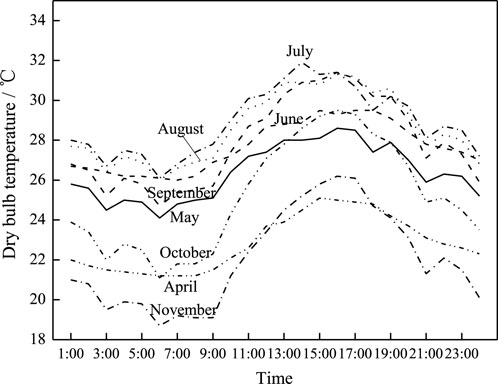
Figure 3. Monthly weighted average dry bulb temperature characteristic.

Figure 4

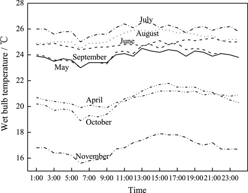
Figure 4. Monthly weighted average wet bulb temperature characteristic.

Figure 5

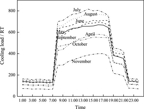
Figure 5. Building monthly weighted average cooling load characteristic.

As is evident from Figure 2, the cooling load of July is highest in the whole year, and the cooling load of November is the lowest. The cooling load curve of April is similar to that of October; the cooling load curve of May is similar to that of September.

5.2 Simulation results validation

Based on the system model and algorithm design, Python was used for programming calculation. Based on the water-cooled central chilling system energy consumption model and its current sequential control logic, nine typical operation conditions were selected to validate the accuracy of the simulation results. The water-cooled central chilling system refrigeration capacity of the nine typical operation conditions were 20%, 30%, 40%, 50%, 60%, 70%, 80%, 90%, and 100% of air conditioning design load, respectively. The 10% air conditioning design load condition did not exist in the field test data, so it was not included in typical operational conditions. The part-load ratio (PLR) is defined as the ratio of the water-cooled central chilling system refrigeration capacity to the air conditioning design load. As depicted in Figure 6, the deviation between the simulated and field test values of the water-cooled central chilling system total energy consumption with sequential control is less than 6.5%. The simulated results show fine precision.

Figure 6

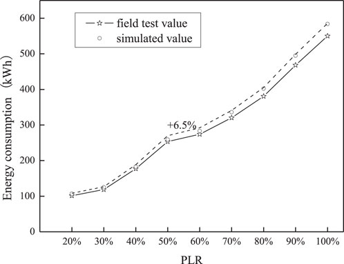
Figure 6. Deviation between simulated and field test values of system total energy consumption.

The refrigeration plant room with the gray wolf optimization algorithm requires the adjustment of operating parameters or hardware, which may affect normal production and make it difficult for enterprises to bear the risk of shutdown or failure. Therefore, owners do not generally allow such adjustment. The difference between sequential control and the gray wolf optimization algorithm is the difference in equipment operating parameters. Total energy consumption simulated results under the above nine typical operation conditions demonstrated fine precision, so the system’s total energy consumption simulated results with the gray wolf optimization algorithm should also show fine precision. The following optimization results analysis is reliable.

5.3 Optimization results analysis

By the programming calculation, the energy consumption and energy efficiency ratio characteristics of the water-cooled central chilling system before and after optimization on the design day are shown in Figure 7. The design day energy consumption of the water-cooled central chilling system was reduced by 8.81% by optimization, and the design day comprehensive energy efficiency ratio was increased from 5.03 to 5.51, yielding an increase of 9.67%. As shown in Figure 8, after optimization, the design day energy consumption of chillers, chilled water pumps, and cooling water pumps were reduced by 508 kWh (8.13%), 104 kWh (12.22%), and 225 kWh (36.95%), respectively, while the energy consumption of the cooling towers increased by 135 kWh (53.15%).

Figure 7

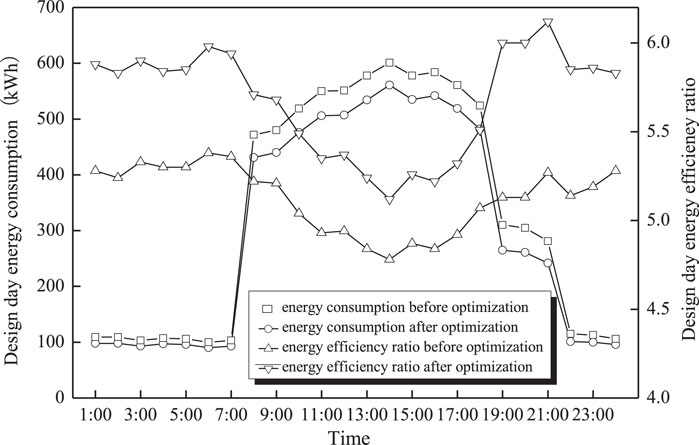
Figure 7. Water-cooled central chilling system energy consumption and energy efficiency comparison between before and after optimization in design day.

Figure 8

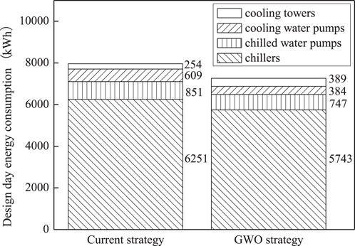
Figure 8. Equipment energy consumption comparison between current and GWO strategy in design day.

As shown in Figure 7, the energy efficiency ratio of the water-cooled central chilling system improved the most by optimization at 19:00, and the energy efficiency ratio improved the least at 06:00. The comparison of energy consumption of each equipment before and after optimization under 06:00 and 19:00 operating conditions on the design day are shown in Figures 9, 10, respectively. The corresponding operating parameters of each piece of equipment before and after optimization are shown in Tables 4 and 5, respectively. It can be seen that the cooling load at 06:00 is very small (Figure 5). At 06:00, the number of devices turned on before optimization is the same as after optimization (Table 4), while the capacity of activated devices after optimization is different from before optimization. Therefore, the energy consumption savings of the water-cooled central chilling system by optimization are not significant (only 3.26%), and the energy efficiency ratio improvement is relatively small (only 3.42%) at 06:00. Similarly, when the cooling load is large, the number of devices turned on before optimization is the same as after optimization, and only the capacity of activated devices can be optimized. At 19:00, the cooling load is relatively moderate, and both the amount and capacity of activated equipment can be optimized (Table 5). Therefore, both energy saving (14.29%) and efficiency improvement (16.79%) are significant through optimization at 19:00.

Figure 9

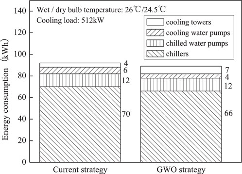
Figure 9. Equipment energy consumption comparison between before and after optimization on design day 06:00.

Figure 10

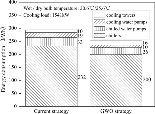
Figure 10. Equipment energy consumption comparison between before and after optimization on design day 19:00.

Table 4

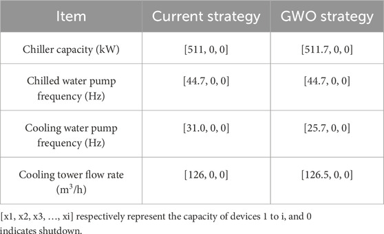
Table 4. Design day 06:00 operating parameters before and after optimization.

Table 5

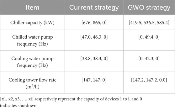
Table 5. Design day 19:00 operating parameters before and after optimization.

As shown in Figure 11, the monthly weighted average energy consumption of the water-cooled central chilling system decreased by 8.47%–16.34% after optimization, and the monthly weighted average energy efficiency ratio increased by 9.25%–19.54%. Of these, as shown in Figure 3, the average weighted cooling load in June, July, and August was relatively high, and the energy-saving space by optimization was very small. The monthly weighted average energy efficiency ratio’s improvement was relatively low. The average weighted cooling load in April was relatively moderate, and energy saving room was large through optimization. The monthly weighted average energy efficiency ratio of April increased the most, reaching 19.54%.

Figure 11

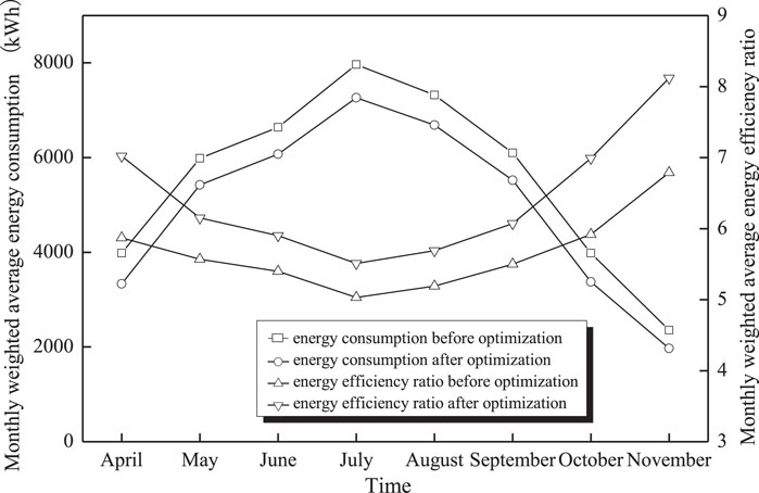
Figure 11. Refrigeration plant room monthly energy consumption and energy efficiency comparison between current and GWO strategy.

The annual energy consumption comparison of each piece of equipment in the water-cooled central chilling system between the current and GWO strategies is shown in Figure 12. The results indicate that the annual total energy consumption of the water-cooled central chilling system decreased by 10.57% by optimization. The energy consumption of chillers, chilled water pumps, and cooling water pumps was saved by 10.35%, 15.51%, and 39.5%, respectively, while the energy consumption of the cooling towers increased by 52.67% after optimization. The comprehensive energy efficiency ratio for the whole year increased from 5.50 to 6.15, an increase of 11.82%. Therefore, the proposed operational optimization strategy for a water-cooled central chilling system based on the grey wolf algorithm is effective.

Figure 12

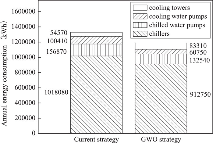
Figure 12. Equipment annual energy consumption comparison between current and GWO strategy.

6 Conclusion

This paper conducted operational optimization research on a water-cooled central chilling system of a commercial office building in Guangzhou based on the grey wolf algorithm. The optimization objective was to maximize the energy efficiency ratio by seeking the optimal number and load distribution of activated chillers, the number and approximation degree of activated cooling towers, and the number and frequency of activated chilled water pumps and activated cooling water pumps. The main finding of this study is that the proposed operational optimization strategy for a water-cooled central chilling system based on the grey wolf algorithm is effective. After optimization, the design day energy efficiency ratio of the water-cooled central chilling system increased from 5.03 to 5.51, an increase of 9.67%, and the annual comprehensive energy efficiency ratio increased from 5.50 to 6.15, an increase of 11.82%.

6.1 Limitation

The limitations of the study is that there is a lack of grey wolf optimization algorithm simulation results verification. Refrigeration plant room with grey wolf optimization algorithm requires adjustment of operating parameters or hardware, which may affect normal production and make it difficult for enterprises to bear the risk of shutdown or failure. So generally, owners do not allow such adjustment. In the future, we will conduct wolf optimization algorithm experiment of the actual water-cooled central chilling system in small building in its spare time.

Data availability statement

The original contributions presented in the study are included in the article/supplementary material; further inquiries can be directed to the corresponding authors.

Author contributions

JY: Data curation, Formal Analysis, Funding acquisition, Investigation, Writing – original draft. DZ: Funding acquisition, Investigation, Methodology, Supervision, Writing – review and editing. AX: Data curation, Investigation, Resources, Writing – review and editing. LG: Project administration, Resources, Writing – review and editing. WZ: Methodology, Software, Validation, Writing – review and editing. YC: Investigation, Methodology, Supervision, Writing – review and editing.

Funding

The author(s) declare that financial support was received for the research and/or publication of this article. The authors gratefully acknowledge the support provided by the Scientific Research Fund of Guangzhou Maritime University under grant no. K42022108 and K42024047.

Conflict of interest

Author AX was employed by Engineering Company Public Office, Nanjing Fiberglass Research & Design Institute Co., Ltd. Author LG was employed by Guangzhou Shijie Energy Saving Technology Co., Ltd.

The remaining authors declare that the research was conducted in the absence of any commercial or financial relationships that could be construed as a potential conflict of interest.

Generative AI statement

The author(s) declare that no Generative AI was used in the creation of this manuscript.

Any alternative text (alt text) provided alongside figures in this article has been generated by Frontiers with the support of artificial intelligence and reasonable efforts have been made to ensure accuracy, including review by the authors wherever possible. If you identify any issues, please contact us.

Publisher’s note

All claims expressed in this article are solely those of the authors and do not necessarily represent those of their affiliated organizations, or those of the publisher, the editors and the reviewers. Any product that may be evaluated in this article, or claim that may be made by its manufacturer, is not guaranteed or endorsed by the publisher.

References

Ali, M., Vukovic, V., Sahir, M. H., and Fontanella, G. (2013). Energy analysis of chilled water system configurations using simulation-based optimization. Energy Build. 59, 111–122. doi:10.1016/j.enbuild.2012.12.011

CrossRef Full Text | Google Scholar

Chan, K. C., Wong, V. T. T., Yow, A. K. F., Yuen, P. L., and Chao, C. Y. H. (2022). Development and performance evaluation of a chiller plant predictive operational control strategy by artificial intelligence. Energy Build. 262, 112017. doi:10.1016/j.enbuild.2022.112017

CrossRef Full Text | Google Scholar

Chen, Y., Hong, T., Luo, X., and Hooper, B. (2019). Development of city buildings data set for urban building energy modeling. Energy Build. 183, 252–265. doi:10.1016/j.enbuild.2018.11.008

CrossRef Full Text | Google Scholar

Chen, Y., Yang, C., Pan, X., and Yan, D. (2020). Design and operation optimization of multi-chiller plants based on energy performance simulation. Energy Build. 222, 110100. doi:10.1016/j.enbuild.2020.110100

CrossRef Full Text | Google Scholar

China Electronic Energy Conservation Technology Association (2024). Technical specification for energy efficiency simulation and optimization control of efficient centralized air conditioning plant room. Beijing: China Electronic Energy Conservation Technology Association.

Google Scholar

Deng, Q., Xu, L., Zhao, T., Hong, X., Shan, X., and Ren, Z. (2022). Cooperative optimization of A refrigeration system with A water-cooled chiller and air-cooled heat pump by coupling BPNN and PSO. Energies 15, 7077. doi:10.3390/en15197077

CrossRef Full Text | Google Scholar

Gao, Z., Yu, J., Zhao, A., Hu, Q., and Yang, S. (2022). Optimal chiller loading by improved parallel particle swarm optimization algorithm for reducing energy consumption. Int. J. Refrig. 136, 61–70. doi:10.1016/j.ijrefrig.2022.01.014

CrossRef Full Text | Google Scholar

Gordon, J. M., and Ng, K. C. (1995). A general thermodynamic model for absorption chillers:Theory and experiment. Heat. Recovery Systems Chp 15 (1), 73–83. doi:10.1016/0890-4332(95)90038-1

CrossRef Full Text | Google Scholar

Harish Kumar, P., and Mageshvaran, R. (2022). Grey wolf optimisation algorithm for solving distribution network reconfiguration considering distributed generators simultaneously. Int. J. Sustain. Energy 41 (11), 2121–2149. doi:10.1080/14786451.2022.2134383

CrossRef Full Text | Google Scholar

Hong, T., Chen, Y., Luo, X., Luo, N., and Lee, S. H. (2020). Ten questions on urban building energy modeling. Build. Environ. 168, 106508. doi:10.1016/j.buildenv.2019.106508

CrossRef Full Text | Google Scholar

Hu, Y., Qin, L., Li, S., Li, X., Li, Y., and Sheng, W. (2024). Optimal chiller loading based on flower pollination algorithm for energy saving. J. Build. Eng. 93, 109884. doi:10.1016/j.jobe.2024.109884

CrossRef Full Text | Google Scholar

Huang, S., Zuo, W., and Sohn, M. D. (2016). Amelioration of the cooling load based chiller sequencing control. Appl. Energy 168, 204–215. doi:10.1016/j.apenergy.2016.01.035

CrossRef Full Text | Google Scholar

Jia, L., Shen, W., and Liu, J. (2021). A review of optimization approaches for controlling water-cooled central cooling systems. Build. Environ. 203, 108100. doi:10.1016/j.buildenv.2021.108100

CrossRef Full Text | Google Scholar

Karami, M., and Wang, L. (2018). Particle Swarm optimization for control operation of an allvariable speed water-cooled chiller plant. Appl. Therm. Eng. 130, 962–978. doi:10.1016/j.applthermaleng.2017.11.037

CrossRef Full Text | Google Scholar

Lee, T. S., and Lu, W. C. (2010). An evaluation of empirically-based models for predicting energy performance of vapor-compression water chillers. Appl. Energy 87 (11), 3486–3493. doi:10.1016/j.apenergy.2010.05.005

CrossRef Full Text | Google Scholar

Liu, X., Huang, B., and Zheng, Y. (2023). Control strategy for dynamic operation of multiple chillers under random load constraints. Energy 270, 126932. doi:10.1016/j.energy.2023.126932

CrossRef Full Text | Google Scholar

Luan, Z. J., Zhang, G. M., Tian, M. C., and Fan, M. x. (2008). Flow resistance and heat transfer characteristics of a new-type plate heat exchanger. J. Hydrodynamics 20 (4), 524–529. doi:10.1016/s1001-6058(08)60089-x

CrossRef Full Text | Google Scholar

Luis, P.-L., Ortiz, J., and Christine, P. (2008). A review on buildings energy consumption information. Energ Build. 40 (3), 394–398. doi:10.1016/j.enbuild.2007.03.007

CrossRef Full Text | Google Scholar

Mirjalili, S., Mirjalili, S. M., and Lewis, A. (2014). Grey wolf optimizer. Adv. Eng. Softw. 69 (3), 46–61. doi:10.1016/j.advengsoft.2013.12.007

CrossRef Full Text | Google Scholar

Rajakumar, S., Siva Satya Sreedhar, P., Kamatchi, S., and Tamilmani, G. (2023). Gray wolf optimization and image enhancement with NLM Algorithm for multimodal medical fusion imaging system. Biomed. Signal Process. Control 85, 104950. doi:10.1016/j.bspc.2023.104950

CrossRef Full Text | Google Scholar

Reddy, T. A., and Andersen, K. (2002). An evaluation of classical steady state off line linear parameter estimation methods applied to chiller performance data. HVAC&R Res. 8 (1), 101–124. doi:10.1080/10789669.2002.10391291

CrossRef Full Text | Google Scholar

Yik, F., and Lam, V. (1998). Chiller models for plant design studies. Build. Serv. Eng. Res. Technol. 19 (4), 233–241. doi:10.1177/014362449801900407

CrossRef Full Text | Google Scholar

Zhuang, C., Wang, S., and Shan, K. (2020). A risk-based robust optimal chiller sequencing control strategy for energy-efficient operation considering measurement uncertainties. Appl. Energy 280, 115983. doi:10.1016/j.apenergy.2020.115983

CrossRef Full Text | Google Scholar