Mathematical modeling describing the performance of open loop multivariable vapor compression chiller model: implications for sustainable HVAC in social housing development

Introduction: This study introduces a simplified multi-variable state-space model of a vapour compression chiller system, focusing on key components such as the condenser and evaporator.

Methods: The model is based on a previously validated state-space framework and has been further developed to generate a transfer function matrix with two inputs (refrigerant and cold carrier flow rates) and two outputs (cooling capacity and outlet temperature). The simplified model offers an accurate yet computationally efficient representation of the system’s dynamics. Simulations of the open-loop system were carried out using SIMULINK/MATLAB software. The results were plotted to validate the model's ability to predict system responses accurately. These simulations encompassed various conditions, including operational changes, fouling on the evaporator, and thermal load fluctuations.

Results: Open-loop simulation results show that the system reaches steady-state values with a response time of approximately 40 seconds for the cold carrier temperature and 70 seconds for cooling capacity. Meanwhile, the system exhibits strong coupling between inputs and outputs, with disturbances such as inlet temperature variations causing oscillations in the cooling capacity.

Discussion: The novelty of this work lies in reducing a complex validated chiller model into a practical two-input, two-output framework, which enables simplified analysis and serves as a robust foundation for advanced multivariable control design. This contribution addresses the critical need for efficient HVAC control strategies in sustainable building applications. This research presents a foundational mathematical model for developing advanced feedback control strategies that can enhance system stability, improve energy efficiency, and support sustainable HVAC operations while maintaining thermal comfort. These advancements are especially relevant for social housing, where energy-efficient HVAC systems are essential for achieving sustainable and resilient building practices in extreme climate conditions.

1 Introduction and related scholarly work

Mathematical models are employed across various fields, including engineering, ecology, agriculture, medicine, and economics, primarily to forecast and regulate the operation of systems in real-world applications (Homod, 2013). Mathematical modelling is, for example, extensively used in construction and civil engineering (Addis, 2020), because replicating large-scale structures like buildings, bridges, or dams in a laboratory is impractical and costly, while modelling provides accurate insights into structural behaviour under various conditions. In the field of building energy management, creating precise and efficient mathematical models of a building’s components is a vital process (Pan et al., 2023). These components include the building envelope, orientation, and building services. Such models are crucial for predicting and optimising performance, especially in energy-intensive services like lighting and Heating, Ventilation, and Air Conditioning (HVAC) systems (Jang et al., 2019). Accurately predicting building service behaviour is crucial for energy-efficient operations. A reliable mathematical model supports optimal decision-making, helping to optimize energy use while ensuring performance.

HVAC systems are responsible for a significant portion of building energy use, often consuming up to 50% of a building’s total energy (Simpeh et al., 2022). They contribute substantially to greenhouse gas emissions, mainly when they operate on fossil fuels, which can harm the environment and exacerbate climate change. According to the International Energy Agency (IEA), energy consumption for air conditioning is projected to increase 4.5 times by 2050 in countries outside the Organisation for Economic Co-operation and Development (OECD), compared to a 1.3 times increase within OECD countries (Goetzler et al., 2016). This increase in demand is driven by higher incomes and better access to air conditioning, especially in developing countries. As a result, the need for HVAC system installations is likely to grow further in the coming years, making these systems even more vital for meeting future energy needs. Consequently, it is imperative to explore methods to decrease energy usage and enhance the efficiency of HVAC systems, thereby diminishing their carbon footprint and contributing to environmental conservation (Kathiravel et al., 2024).

To reduce energy use in buildings, indirect approaches such as passive design strategies are often recommended (Palmero-marrero & Oliveira, 2010). These strategies include features like improved insulation, shading devices, and green roofs, which help minimise energy demand for heating and cooling (Castleton et al., 2010). Additionally, cooling methods, including enhanced insulation, green roofs, and photovoltaic systems, have been explored to improve energy efficiency (Touqan et al., 2017). Retrofitting buildings to improve energy efficiency and sustainability is another important focus in building design (Ma et al., 2012). Despite these efforts to reduce energy consumption, HVAC systems remain essential in maintaining high levels of thermal comfort and air quality (Asim et al., 2022), which cannot be fully achieved through passive cooling strategies alone.

HVAC systems are inherently complex due to their multicomponent structure and strong interdependencies among elements such as evaporators, compressor and condensers, making their modelling and control a challenging task (Seyam, 2018; Touqan and Ameer, 2024). Inadequate control design can lead to increased energy consumption, frequent maintenance, poor performance, and user dissatisfaction (Angel, 2011). Enhancing system efficiency requires the integration of multidisciplinary knowledge through Systems Engineering, which applies structured methodologies to optimise performance (Subbaram Naidu and Rieger, 2011). Central to this process is the development of accurate and dynamic mathematical models that reliably represent system behaviour, forming the basis for effective control strategies (Li et al., 2010; Whalley and Abdul-Ameer, 2011). Such models enable the precise regulation of system outputs, thereby reducing energy waste and improving operational efficiency in real-time scenarios.

To contextualise the investigation of HVAC systems’ performance, they are vital for comfort in extreme-heat social housing, where high energy bills strain low-income residents. In the Arabian Gulf (>40°C), inefficient HVAC units worsen energy poverty and emissions; thus, despite passive design and retrofit efforts, dynamic modelling and control remain essential for maximizing efficiency without compromising comfort.

Hence, the motivation for this study is to derive a simplified and reliable mathematical model. While prior works validated a high-order state-space model (Yao et al., 2013), its complexity challenges real-time control applications. Computational efficiency is paramount for adaptive HVAC control in dynamic environments, yet most MIMO models either oversimplify coupling effects or lack experimental validation. A simplified two-input, two-output model that preserves essential dynamics can address this gap, facilitating deployment in resource-constrained contexts such as social housing.

Therefore, the research objectives can be derived from addressing the following research question: How can a simplified multivariable model enhance control efficiency and energy performance in HVAC systems for social housing? So, the objectives of the study are:

i. Deriving a reduced-order transfer function matrix from (Yao et al., 2013) validated state-space framework, focusing on refrigerant and chilled water flow rates as inputs. A transfer function, obtained through Laplace transforms, turns time-domain dynamics into an algebraic input-output relation. For the chiller it maps refrigerant-flow changes to cooling capacity, capturing delays and response shape.

ii. Validating the model’s open-loop dynamics under disturbances (e.g., fouling, load variations) through SIMULINK software to identify control challenges.

iii. Discussing its utility as a foundation for multivariable feedback control, emphasising decoupling and stability in extreme climates.

This study aims to develop and validate a simplified two-input, two-output transfer function model of a vapour compression chiller, derived from a high-order state-space system. The model maintains key dynamic behaviour, improves computational efficiency, and supports real-time control. It facilitates advanced feedback strategies to boost stability, energy efficiency, and performance, especially in extreme climates. This model underpins cost-effective, resilient HVAC solutions aligned with energy and comfort goals in sustainable social housing.

Given the focus on energy-efficient HVAC operation and control-oriented modelling, the literature review situates the research within existing scholarly work. It outlines key modelling methods for HVAC, highlighting their advantages, limitations, and suitability for streamlined control models. This forms the basis for the methodological choices in this study.

Some researchers, especially those in (Homod, 2013; Afram and Janabi-Sharifi, 2014), have reviewed three distinct approaches to mathematical modelling. The first is the physics-based model, also known as the “white box model.” This model requires a deep understanding of the underlying processes. In the case of HVAC systems, physics-based models usually rely on equations related to mass and energy conservation, as well as principles of heat transfer. This approach necessitates comprehensive knowledge of the system being analysed. A significant benefit of physics-based modelling is its capacity to predict the system’s behaviour and estimate various outputs accurately. For instance, the research in (Ali, 2019) developed a mathematical load model for major household appliances, particularly air conditioners (ACs), based on physical and operational characteristics. Physics-based models, grounded in thermodynamic principles, offer high prediction accuracy and detailed system representation (Jorissen et al., 2021).

However, their complexity can limit real-time control applications (Silvestri et al., 2023; Zhao et al., 2021). These models are computationally demanding and require significant development effort (Y. Li et al., 2022). Moreover, while the model is built on fundamental physical relationships and validated against real data, it lacks a transparent methodology for parameter identification and uncertainty quantification, which are key requirements in white box modelling as emphasised by (Bacher and Madsen, 2011). Meanwhile, these models often encounter challenges in adapting to real-time control applications due to their inherent complexity and rigidity. Furthermore, they exhibit limited robustness when applied to systems with varying operating conditions, thereby reducing their practicality for adaptive HVAC control strategies necessary in dynamic environments such as social housing.

The second modelling approach is data-driven, often called a “black box model”. Studies such as those by (Ma et al., 2015; Zlatanović et al., 2011) have applied this method for HVAC systems, which are inherently complex with numerous parameters that make physics-based modelling difficult. Data-driven models can model complicated behaviour system (Zhou et al., 2017) and (Zhou et al., 2016). These models are beneficial for managing nonlinearities and are simpler to compute than traditional physical-based methods. However, the accuracy of these models can be significantly impacted by poor data quality, which is prevalent in large databases. Despite their advantages, data-driven methods face challenges such as poor interpretability and conservative predictions in extreme cases (Wu and Xue, 2024). In the same context, the study by (Zhang, 2023) provides a comprehensive critique of machine learning-driven building control systems, highlighting that although machine learning demonstrates potential in optimising energy consumption, considerable challenges persist, particularly concerning data quality, model interpretability, and the ability to generalise to new operational conditions. This highlights an important challenge in current data-driven methods, which often work as mysterious “black boxes” and can be difficult to validate in many real-world settings.

The third approach to modelling is the hybrid method, also known as the “grey box model,” which combines both data-driven and physics-based techniques. In this method, physics-based equations are used to develop the core model, while actual data helps to identify key parameter values. These data can be sourced from system specifications provided by manufacturers or from the system commissioning process. For example, in the study (Jin et al., 2011), a grey box model was created for cooling coil units, incorporating heat transfer equations and energy and mass balance principles. The model streamlined the calibration process by focusing on six parameters that represented the unit’s nonlinear characteristics. These parameters were derived from manufacturer data or experimental findings. The grey box approach faces challenges in parameter calibration and balancing physical insight with computational efficiency. Calibration is sensitive to data quality and quantity, with longer, diverse datasets improving model generalisation and accuracy (Murphy et al., 2021). The process requires substantial domain expertise to manage effectively. While grey-box models can provide physical interpretations of parameters, they may not fully capture parameter interactions or uncertainties (Pavlak et al., 2014). Despite these limitations, grey-box modelling can significantly reduce labour input compared to white-box approaches (Murphy et al., 2021). Overall, grey-box modelling remains the most effective modelling approach, offering a compromise between physical insight and data-driven efficiency. Still, it requires careful consideration of calibration strategies and data quality.

Traditionally, HVAC research has centred on single-input, single-output (SISO) models that isolate components such as compressors, cooling coils, air-handling units, or building envelopes (Li et al., 2014; Lapinskiene and Martinaitis, 2013). However, real HVAC systems are inherently multivariable, featuring several interacting inputs and outputs. Given the high energy consumption of these systems, it is more practical and representative to model them as multiple-input, multiple-output (MIMO) systems. This approach, where a change in one input affects multiple outputs, better captures the system’s complexity and energy demands, as discussed in (Hassan and Al-Samarraie, 2022), offering significant potential to optimize performance by manipulating various system parameters.

Recent research underscores the importance of MIMO modeling for HVAC systems, as it provides a more comprehensive representation of their complex internal interactions. MIMO modelling has been shown to provide a more comprehensive representation of the complex interactions within HVAC systems (Abdo-Allah et al., 2018; Abdo-Allah et al., 2017). State-space approaches have been effectively utilized to develop MIMO models for HVAC systems, facilitating more robust control system design and analysis (Abdo-Allah et al., 2018). Furthermore, advanced control strategies, including Direct Nyquist Array (DNA) and PID controllers, have been successfully implemented in MIMO HVAC models, leading to improved system performance and effective decoupling of system outputs (Touqan et al., 2022).

Most HVAC studies still rely on SISO models that overlook the strong inter-variable couplings of real systems. Although grey-box MIMO models offer richer dynamics, existing work is too computationally demanding for real-time control, highlighting a research gap. This research addresses this by extracting a validated high-order chiller model into a simplified grey-box 2 × 2 formulation, enabling practical multivariable control that reduces energy use, capturing the key dynamical system behaviour and enhances comfort in high-energy consumption systems.

2 Research methodology

This study builds upon the rigorously validated state-space model of a vapour compression chiller system established by (Yao et al., 2013). It will be developing a more concise, two-input, two-output multivariable model; this research accurately reflects the system’s dynamic behaviour. The model, which integrates essential components such as the condenser and evaporator based on fundamental principles of mass and energy conservation and heat transfer, aims to provide a computationally efficient yet realistic representation of chiller operations. It will indeed derive a simplified reduced-order model that still captures the same transient and steady-state behaviour of the original high-order model. Instead of presenting the detailed equations from the original work, this research focuses specifically on the sets of state equations and output equations only provided by (Yao et al., 2013), avoiding redundancy and duplication of effort.

2.1 Chiller system description

In this section, the chiller employed by (Yao et al., 2013) will be reviewed to identify the system components, inputs and outputs that will be selected for the simplified mathematical model process. It consists of four main components: the compressor, condenser, expansion device, and evaporator, as illustrated in Figure 1. Additionally, it includes several auxiliary elements, such as the chiller water pump. This figure represents the single-stage cycle, which serves as a standard model for practical refrigeration systems. Within this cycle, the refrigerant absorbs heat from the air-conditioned space via the evaporator, where its heat capacity is assumed to remain constant throughout the loop. Upon entering the compressor, the refrigerant’s pressure and temperature are significantly increased. In the condenser, the refrigerant undergoes a heat rejection process, during which its temperature decreases linearly due to heat transfer. The cycle concludes with the refrigerant passing through the expansion device, where it undergoes a pressure drop and further cooling.

Figure 1

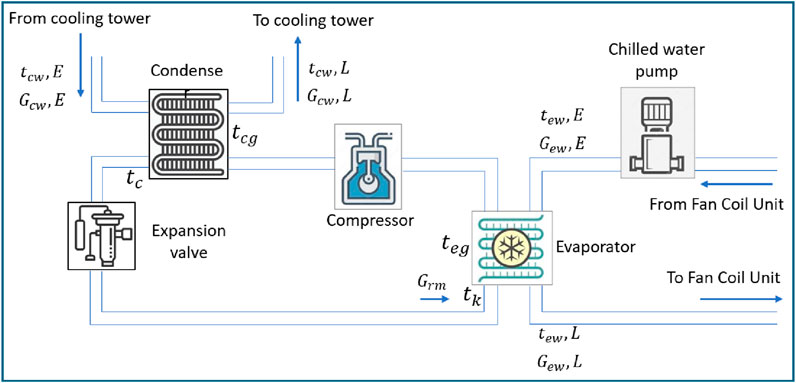
Figure 1. Vapour compression liquid chiller plant.

In the refrigeration cycle, the chilled water (cold carrier fluid) enters the evaporator at a temperature $t_{ew},E\left(t\right)$ after absorbing heat from the air-conditioned space. Inside the evaporator, the chilled water transfers this absorbed heat to the refrigerant, exiting at a reduced temperature $t_{ew},L\left(t\right)$. The cooled water then carries the cooling effect back to the indoor environment. It is subsequently routed to the Fan Coil Unit (FCU), where a blower fan distributes the cool air into the space. However, the FCU is not included in this model or analysis.

As the refrigerant moves through the compressor, its pressure and temperature rise significantly, preparing it for the condensation stage. In the condenser, the refrigerant releases the heat absorbed during the evaporation phase. This heat rejection is supported by the condenser coolant, which facilitates efficient thermal exchange. The inlet and outlet temperatures of the condenser coolant are represented by $t_{cw},E\left(t\right)$ and $t_{cw},L\left(t\right)$, respectively. This heat transfer process gradually lowers the refrigerant’s temperature. The cycle is completed as the refrigerant passes through the expansion device, where its pressure drops and cools further, making it ready to re-enter the evaporator and commencing a new cycle.

2.2 Chiller mathematical model

A state-space model of the vapor compression chiller system provides a mathematical framework to describe the system’s dynamic behavior through its inputs, state variables, and outputs. This model is based on the fundamental physical principles governing the chiller, including mass and energy conservation. It is a representation in a structured matrix form, effectively capturing the interactions and dynamic relationships between the various system components.

The standard state space representation is given by the following pair of equations

$\frac{dx}{dt}=Ax\left(t\right)+Bu\left(t\right)(1)$

$y\left(t\right)=Cx\left(t\right)+Du\left(t\right)(2)$

Where:

$x\left(t\right):$ is the chiller states vector and equals to ${\left[t_c,t_{cw}L,t_{cg},t_k,t_{ew}L,t_{eg}\right]}^T$

$A:$ The square matrix represents the internal dynamics of the system by defining how the current state variables influence their rates of change. Its elements describe the interactions between different states, such as the effect of temperature at one stage on another within the system.

$B:$ The input matrix shows how external inputs affect the rate of change of state variables. Its elements reflect the influence of inputs, such as refrigerant mass flow rate or coolant flow rate, on system states like temperatures.

$u\left(t\right):$ The input vector that represents the external inputs to the system (e.g., external temperatures and fluid mass flow rates) and equals to ${\left[t_{cw}E,G_{cw}E,t_{ew}E,G_{ew}E,G_{rm}\right]}^T$.

$y\left(t\right):$ The output vector represents the measurable outputs of the system and is equal to ${\left[t_{cw},L,G_{cw},L,t_{ew},L,G_{ew},L,W_{w,com},Q_c,COP\right]}^T$.

$C:$ This is the output matrix that maps the state variables to the system outputs. It defines how the states directly influence the outputs. The elements of this matrix describe how the internal states of the chiller system influence measurable outputs.

$D:$ This is the direct transmission matrix that maps the inputs directly to the outputs, accounting for any immediate or direct effect of inputs on outputs. The elements of this matrix describe how external inputs (e.g., compressor speed, valve position) directly and immediately affect these outputs.

Equations 3–31 present the sequential mathematical derivations that conclude the final simplified chiller multivariable input-output relationship in matrix form. Based on (Yao et al., 2013), the state space and output equations can be extracted and developed as follows:

$\frac{d{t}_c}{dt}=-5.1837t_c+5.179t_{cg}+27.1594G_{rm}(3)$

$\frac{d{t}_{cw},L}{dt}=-1.44962t_{cw},L+2.0831t_{cg}-0.5870t_{cw},E-0.0124G_{cw},E(4)$

$\frac{d{t}_{cg}}{dt}=1.0117t_c+0.2026t_{cw},L-1.4169t_{cg}+0.2026t_{cw},E-0.9294G_{cw},E(5)$

$\frac{d{t}_k}{dt}=0.0540t_c-30.6731t_k+30.6338t_{eg}-56.8937G_{rm}(6)$

$\frac{d{t}_{ew},L}{dt}=-2.1864t_{ew},L+1.8934t_{eg}+0.0454t_{cw},E+5.9930G_{ew},E(7)$

$\frac{d{t}_{eg}}{dt}=4.4032t_k+0.1520t_{ew},L-4.7073t_{eg}+0.1508t_{cw},E-0.2387G_{ew},E(8)$

$t_{cw},L=t_{cw},L(9)$

$G_{cw},L=G_{cw},E(10)$

$t_{ew},L=t_{ew},L(11)$

$G_{ew},L=G_{ew},L(12)$

$W_{w,com}=136.1257t_c-125.341t_k(13)$

$Q_c=-172.1875t_c+ 125.34t_k+27502G_{rm}(14)$

$COP=-0.2992t_c+0.2662t_k+181333G_{rm}(15)$

Mapping the equations from Equations 3 to 15 into the state-space equations defined in (1) and (2) results in the matrix representation of the state-space model for the chiller system as follows:

$\begin{array}{c}\frac{d}{dt}\left[\begin{array}{c}{t}_c\\ t_{cw},L\\ t_{cg}\\ t_k\\ t_{ew},L\\ t_{eg}\end{array}\right]=\left[\begin{array}{cccccc}-5.1837& 0& 5.1790& 0& 0& 0\\ 0& -1.44962& 2.0831& 0& 0& 0\\ 1.0117& 0.2026& -1.4169& 0& 0& 0\\ 0.0540& 0& 0& -30.6731& 0& 30.6338\\ 0& 0& 0& 0& -2.1864& 1.8934\\ 0& 0& 0& 4.4032& 0.1520& -4.7073\end{array}\right]\left[\begin{array}{c}{t}_c\\ t_{cw},L\\ t_{cg}\\ t_k\\ t_{ew},L\\ t_{eg}\end{array}\right]\\ +\left[\begin{array}{ccccc}0& 0& 0& 0& 27.1594\\ -0.5870& -0.0124& 0& 0& 0\\ 0.2026& -0.9294& 0& 0& 0\\ 0& 0& 0& 0& -56.8937\\ 0& 0& 0.0454& 5.9930& 0\\ 0& 0& 0.1508& -0.2387& 0\end{array}\right]\left[\begin{array}{c}{t}_{cw},E\\ G_{cw},E\\ t_{ew},E\\ G_{ew},E\\ G_{rm}\end{array}\right]\end{array}(16)$

$\begin{array}{c}\left[\begin{array}{c}{t}_{cw},L\\ G_{cw},L\\ t_{ew},L\\ G_{ew},L\\ W_{w,com}\\ Q_c\\ COP\end{array}\right]=\left[\begin{array}{cccccc}0& 1& 0& 0& 0& 0\\ 0& 0& 0& 0& 0& 0\\ 0& 0& 0& 0& 1& 0\\ 0& 0& 0& 0& 0& 0\\ 136.1257& 0& 0& -125.341& 0& 0\\ -172.1875& 0& 0& 125.341& 0& 0\\ -0.2992& 0& 0& 0.2662& 0& 0\end{array}\right]\left[\begin{array}{c}{t}_c\\ t_{cw},L\\ t_{cg}\\ t_k\\ t_{ew},L\\ t_{eg}\end{array}\right]\\ +\left[\begin{array}{ccccc}0& 0& 0& 0& 0\\ 0& 1& 0& 0& 0\\ 0& 0& 0& 0& 0\\ 0& 0& 0& 1& 0\\ 0& 0& 0& 0& 0\\ 0& 0& 0& 0& 27502\\ 0& 0& 0& 0& 181333\end{array}\right]\left[\begin{array}{c}{t}_{cw},E\\ G_{cw},E\\ t_{ew},E\\ G_{ew},E\\ G_{rm}\end{array}\right]\end{array}(17)$

It can be easily concluded that the state space matrices are

$A=\left[\begin{array}{cccccc}-5.1837& 0& 5.1790& 0& 0& 0\\ 0& -1.44962& 2.0831& 0& 0& 0\\ 1.0117& 0.2026& -1.4169& 0& 0& 0\\ 0.0540& 0& 0& -30.6731& 0& 30.6338\\ 0& 0& 0& 0& -2.1864& 1.8934\\ 0& 0& 0& 4.4032& 0.1520& -4.7073\end{array}\right](18)$

$B=\left[\begin{array}{ccccc}0& 0& 0& 0& 27.1594\\ -0.5870& -0.0124& 0& 0& 0\\ 0.2026& -0.9294& 0& 0& 0\\ 0& 0& 0& 0& -56.8937\\ 0& 0& 0.0454& 5.9930& 0\\ 0& 0& 0.1508& -0.2387& 0\end{array}\right](19)$

$C=\left[\begin{array}{cccccc}0& 1& 0& 0& 0& 0\\ 0& 0& 0& 0& 0& 0\\ 0& 0& 0& 0& 1& 0\\ 0& 0& 0& 0& 0& 0\\ 136.1257& 0& 0& -125.341& 0& 0\\ -172.1875& 0& 0& 125.341& 0& 0\\ -0.2992& 0& 0& 0.2662& 0& 0\end{array}\right](20)$

$D=\left[\begin{array}{ccccc}0& 0& 0& 0& 0\\ 0& 1& 0& 0& 0\\ 0& 0& 0& 0& 0\\ 0& 0& 0& 1& 0\\ 0& 0& 0& 0& 0\\ 0& 0& 0& 0& 27502\\ 0& 0& 0& 0& 181333\end{array}\right](21)$

2.3 Transfer function matrix

To obtain the transfer function matrix, we take the Laplace transform of both the state and output equations, assuming zero initial conditions (i.e., $x\left(0\right)=0$):

The Laplace transform of the state Equation 1 becomes:

$sx\left(s\right)=Ax\left(s\right)+Bu\left(s\right)(22)$

The Laplace transform of the output Equation 2 becomes:

$y\left(s\right)=Cx\left(s\right)+Du\left(s\right)(23)$

where:

$x\left(s\right)$ is the Laplace transform of the state vector $x\left(t\right)$, $y\left(s\right)$ is the Laplace transform of the output vector $y\left(t\right)$, $u\left(s\right)$ is the Laplace transform of the input vector $u\left(t\right)$, s is the Laplace variable.

Rearranging Equation 22 to solve for $x\left(s\right)$, we get:

$x\left(s\right)={\left(sI-A\right)}^{-1}Bu\left(s\right)(24)$

where $I$ is the identity matrix of appropriate dimensions, and ${\left(sI-A\right)}^{-1}$ is the inverse of the $\left(sI-A\right)$.

Substituting $x\left(s\right)$ into the output Equation 23 yields:

$Y\left(s\right)=C{\left(sI-A\right)}^{-1}Bu\left(s\right)+Du\left(s\right)(25)$

The transfer function matrix $G\left(s\right)$ is defined as the ratio of the output to the input in the Laplace domain:

$G\left(s\right)=\frac{Y\left(s\right)}{u\left(s\right)}={C\left(sI-A\right)}^{-1}\mathrm{B}+\mathrm{D}(26)$

Equation 26 is the transfer function matrix of the system, where each element of $G\left(s\right)$ represents the transfer function from each input to each output. Substituting matrices $A,B,C$ and $D$ in Equation 26 aiming to calculate the transfer function matrix with the aid of MATLAB yields

$\mathrm{G}\left(\mathrm{s}\right)=\left[\begin{array}{ccccc}{\mathrm{g}}_{11}\left(s\right)& {\mathrm{g}}_{12}\left(s\right)& {\mathrm{g}}_{13}\left(s\right)& {\mathrm{g}}_{14}\left(s\right)& {\mathrm{g}}_{15}\left(s\right)\\ {\mathrm{g}}_{21}\left(s\right)& {\mathrm{g}}_{22}\left(s\right)& {\mathrm{g}}_{23}\left(s\right)& {\mathrm{g}}_{24}\left(s\right)& {\mathrm{g}}_{25}\left(s\right)\\ {\mathrm{g}}_{31}\left(s\right)& {\mathrm{g}}_{32}\left(s\right)& {\mathrm{g}}_{33}\left(s\right)& {\mathrm{g}}_{34}\left(s\right)& {\mathrm{g}}_{35}\left(s\right)\\ {\mathrm{g}}_{41}\left(s\right)& {\mathrm{g}}_{42}\left(s\right)& {\mathrm{g}}_{43}\left(s\right)& {\mathrm{g}}_{44}\left(s\right)& {\mathrm{g}}_{45}\left(s\right)\\ {\mathrm{g}}_{51}\left(s\right)& {\mathrm{g}}_{52}\left(s\right)& {\mathrm{g}}_{53}\left(s\right)& {\mathrm{g}}_{54}\left(s\right)& {\mathrm{g}}_{55}\left(s\right)\\ {\mathrm{g}}_{61}\left(s\right)& {\mathrm{g}}_{62}\left(s\right)& {\mathrm{g}}_{63}\left(s\right)& {\mathrm{g}}_{64}\left(s\right)& {\mathrm{g}}_{65}\left(s\right)\\ {\mathrm{g}}_{71}\left(s\right)& {\mathrm{g}}_{72}\left(s\right)& {\mathrm{g}}_{73}\left(s\right)& {\mathrm{g}}_{74}\left(s\right)& {\mathrm{g}}_{75}\left(s\right)\end{array}\right](27)$

where

${\mathrm{g}}_{11}\left(\mathrm{s}\right)=\frac{-0.587{\mathrm{s}}^2-3.453\mathrm{s}+0.952}{{\mathrm{s}}^3+8.097{\mathrm{s}}^2+11.56\mathrm{s}+0.9621}$

${\mathrm{g}}_{12}\left(\mathrm{s}\right)=\frac{-0.0142{\mathrm{s}}^2-2.03\mathrm{s}-10.07}{{\mathrm{s}}^3+8.097{\mathrm{s}}^2+11.56\mathrm{s}+0.9621}$

${\mathrm{g}}_{13}\left(s\right)={\mathrm{g}}_{14}\left(s\right)=0$

${\mathrm{g}}_{15}\left(s\right)=\frac{57.24}{s^3+8.097s^2+11.56s+0.9621}$

${\mathrm{g}}_{21}\left(s\right)={\mathrm{g}}_{23}\left(s\right)={\mathrm{g}}_{24}\left(s\right)={\mathrm{g}}_{25}\left(s\right)=0$

${\mathrm{g}}_{22}\left(s\right)=1$

${\mathrm{g}}_{31}\left(s\right)=\frac{0.4724\mathrm{s}+0.4295}{{\mathrm{s}}^6+45.66{\mathrm{s}}^5+402.3{\mathrm{s}}^4+1148{\mathrm{s}}^3+1134{\mathrm{s}}^2+221.4\mathrm{s}+11.49}$

${\mathrm{g}}_{32}\left(s\right)=\frac{-2.167\mathrm{s}-3.249}{{\mathrm{s}}^6+45.66{\mathrm{s}}^5+402.3{\mathrm{s}}^4+1148{\mathrm{s}}^3+1134{\mathrm{s}}^2+221.4\mathrm{s}+11.49}$

${\mathrm{g}}_{33}\left(s\right)=\frac{0.0454{\mathrm{s}}^2+1.892\mathrm{s}+9.189}{{\mathrm{s}}^3+37.57{\mathrm{s}}^2+86.57\mathrm{s}+11.94}$

${\mathrm{g}}_{34}\left(s\right)=\frac{5.993\mathrm{s}+1.227}{{\mathrm{s}}^2+2.456\mathrm{s}+0.3402}$

${\mathrm{g}}_{35}\left(s\right)=\frac{-474.3s^2-3010s-252.4}{s^5+43.94s^4+326.4s^3+584.3s^2+124.3s+6.653}$

${\mathrm{g}}_{41}\left(s\right)={\mathrm{g}}_{42}\left(s\right)={\mathrm{g}}_{43}\left(s\right)={\mathrm{g}}_{45}\left(s\right)=0$

${\mathrm{g}}_{44}\left(s\right)=1$

${\mathrm{g}}_{51}\left(s\right)=\frac{142.8s^3+5159s^2+5281s+644.1}{s^5+43.36s^4+302.3s^3+450.9s^2+93.85s+4.987}$

${\mathrm{g}}_{52}\left(s\right)=\frac{-655.2s^3-2.405e04s^2-3.784e04s-4872}{s^5+43.35s^4+302.1s^3+450s^2+93.66s+4.976}$

${\mathrm{g}}_{53}\left(s\right)=\frac{-579s-1292}{s^3+37.57s^2+86.57s+11.94}$

${\mathrm{g}}_{54}\left(s\right)=\frac{916.5s-1494}{s^3+37.57s^2+86.57s+11.94}$

${\mathrm{g}}_{55}\left(s\right)=\frac{1.083e04s^5+2.564e05s^4+1.281e06s^3+2.359e06s^2+1.536e06s+1.405e05}{s^6+45.66s^5+402.3s^4+1148s^3+1134s^2+221.4s+11.49}$

${\mathrm{g}}_{61}\left(s\right)=\frac{-180.7s^2-190s-23.44}{s^4+8.246s^3+12.77s^2+2.669s+0.142}$

${\mathrm{g}}_{62}\left(s\right)=\frac{828.8s^2+1361s+177.3}{s^4+8.246s^3+12.76s^2+2.669s+0.142}$

${\mathrm{g}}_{63}\left(s\right)=\frac{579s+1292}{s^3+37.57s^2+86.57s+11.94}$

${\mathrm{g}}_{64}\left(s\right)=\frac{-916.5s+1494}{s^3+37.57s^2+86.57s+11.94}$

${\mathrm{g}}_{65}\left(s\right)=\frac{27502s^5+1.181e06s^4+8.045e06s^3+1.154e07s^2+1.867e06s+6.75e04}{s^5+43.36s^4+302.2s^3+450.4s^2+93.73s+4.978}$

${\mathrm{g}}_{71}\left(s\right)=\frac{-0.3139s^3-11.34s^2-11.61s-1.41}{s^5+43.35s^4+302.1s^3+450s^2+93.65s+4.976}$

${\mathrm{g}}_{72}\left(s\right)=\frac{1.44s^3+52.87s^2+83.18s+10.72}{s^5+43.36s^4+302.3s^3+450.8s^2+93.81s+4.981}$

${\mathrm{g}}_{73}\left(s\right)=\frac{1.23s+2.745}{s^3+37.57s^2+86.57s+11.94}$

${\mathrm{g}}_{74}\left(s\right)=\frac{-1.947s+3.173}{s^3+37.57s^2+86.57s+11.94}$

${\mathrm{g}}_{75}\left(s\right)=\frac{181333s^2+4.28e04s+2369}{s^2+0.236s+0.01307}$

So that input-output equation in matrix form is given by:

$\left[\begin{array}{c}{t}_{cw},L\\ G_{cw},L\\ t_{ew},L\\ G_{ew},L\\ W_{w,com}\\ Q_c\\ COP\end{array}\right]=\left[\begin{array}{ccccc}{\mathrm{g}}_{11}\left(s\right)& {\mathrm{g}}_{12}\left(s\right)& {\mathrm{g}}_{13}\left(s\right)& {\mathrm{g}}_{14}\left(s\right)& {\mathrm{g}}_{15}\left(s\right)\\ {\mathrm{g}}_{21}\left(s\right)& {\mathrm{g}}_{22}\left(s\right)& {\mathrm{g}}_{23}\left(s\right)& {\mathrm{g}}_{24}\left(s\right)& {\mathrm{g}}_{25}\left(s\right)\\ {\mathrm{g}}_{31}\left(s\right)& {\mathrm{g}}_{32}\left(s\right)& {\mathrm{g}}_{33}\left(s\right)& {\mathrm{g}}_{34}\left(s\right)& {\mathrm{g}}_{35}\left(s\right)\\ {\mathrm{g}}_{41}\left(s\right)& {\mathrm{g}}_{42}\left(s\right)& {\mathrm{g}}_{43}\left(s\right)& {\mathrm{g}}_{44}\left(s\right)& {\mathrm{g}}_{45}\left(s\right)\\ {\mathrm{g}}_{51}\left(s\right)& {\mathrm{g}}_{52}\left(s\right)& {\mathrm{g}}_{53}\left(s\right)& {\mathrm{g}}_{54}\left(s\right)& {\mathrm{g}}_{55}\left(s\right)\\ {\mathrm{g}}_{61}\left(s\right)& {\mathrm{g}}_{62}\left(s\right)& {\mathrm{g}}_{63}\left(s\right)& {\mathrm{g}}_{64}\left(s\right)& {\mathrm{g}}_{65}\left(s\right)\\ {\mathrm{g}}_{71}\left(s\right)& {\mathrm{g}}_{72}\left(s\right)& {\mathrm{g}}_{73}\left(s\right)& {\mathrm{g}}_{74}\left(s\right)& {\mathrm{g}}_{75}\left(s\right)\end{array}\right]\left[\begin{array}{c}{t}_{cw},E\\ G_{cw},E\\ t_{ew},E\\ G_{ew},E\\ G_{rm}\end{array}\right](28)$

2.4 Chiller 2 inputs −2 outputs model

The chiller system detailed in (Yao et al., 2013), with five inputs and seven outputs, illustrates significant complexity. While such a model as open loop set up can provide detailed insights, it also poses challenges like increased computational demands and calibration difficulties when applying a multivariable control strategy. Simplifying the model by selecting fewer, strategically chosen inputs and outputs can reduce complexity while maintaining proper system functionality. The condenser and evaporator are key components in the chiller system, where heat absorption and rejection occur. Simplifying the model by focusing on just two inputs and two outputs related to these components is an effective way to reduce the system’s complexity. However, all the five system inputs can be incorporated in this configuration by considering them either as disturbances or held constant under application of a multivariable control strategy. This approach ensures that the model retains its core functionality while becoming more manageable for analysis and control, making it easier to work with while still capturing the essential thermal processes.

To simplify the model, the chosen input-output pairs are: the refrigerant mass flow rate $G_{rm}\left(t\right)$, which impacts the chiller’s cooling capacity $Q_c\left(t\right)$, and the mass flow rate of the chilled water $G_{ew},E\left(t\right)$, which affects the temperature of the chilled water $t_{ew,L}\left(t\right)$. This selection is practical and follows the physical principles of chiller operation. The refrigerant mass flow rate, controlled by the voltage applied on the compressor, directly affects the cooling capacity by influencing the heat transfer efficiency in the evaporator. Similarly, the chilled water flow rate, controlled by the voltage applied on the chilled water pump, determines the outlet temperature $t_{ew},L\left(t\right)$ by regulating the heat absorption rate. These outputs are measurable and critical for monitoring performance so that $Q_c\left(t\right)$ ensures the cooling demand is met, while $t_{ew},L\left(t\right)$ indicates the cooling effect on the indoor thermal load.

It is worthy to mention that when applying advanced control techniques, the other inputs, namely, $t_{cw},E\left(t\right)$, $t_{ew},E\left(t\right)$ can be considered as disturbances and $G_{cw},E\left(t\right)$ can be held constant. It is also important to highlight that adding more inputs and outputs beyond a 2-inputs-2-outputs setup can make the system more complicated without providing significant performance benefits. Such a configuration would need additional sensors, actuators, and computational power, which might increase energy usage without improving the chiller’s main functions of heat rejection and absorption. Using a two-inputs, two-outputs approach concentrates on the most important variables, ensuring effective control while using fewer resources. This simple design lowers the chances of inefficiency or instability, helping to improve energy efficiency by focusing efforts where they are most beneficial.

Based on Equation 28, the two-input, two-output equations that define a multivariable chiller open loop as simplified model can be extracted as:

$t_{ew},L={\mathrm{g}}_{31}\left(s\right)t_{cw},E+{\mathrm{g}}_{32}\left(s\right)G_{cw},E+{\mathrm{g}}_{33}\left(s\right)t_{ew},E+{\mathrm{g}}_{34}\left(s\right)G_{ew},E+{\mathrm{g}}_{35}\left(s\right)G_{rm}(29)$

$Q_c={\mathrm{g}}_{61}\left(s\right)t_{cw},E+{\mathrm{g}}_{62}\left(s\right)G_{cw},E+{\mathrm{g}}_{63}\left(s\right)t_{ew},E+{\mathrm{g}}_{64}\left(s\right)G_{ew},E+{\mathrm{g}}_{65}\left(s\right)G_{rm}(30)$

The multivariable input-output relationship in matrix form can be written as:

$\left[\begin{array}{c}{t}_{ew},L\left(s\right)\\ Q_c\end{array}\right]=\left[\begin{array}{cc}{\mathrm{g}}_{34}\left(s\right)& {\mathrm{g}}_{35}\left(s\right)\\ {\mathrm{g}}_{64}\left(s\right)& {\mathrm{g}}_{65}\left(s\right)\end{array}\right]\left[\begin{array}{c}{G}_{ew},E\left(s\right)\\ G_{rm}\left(s\right)\end{array}\right]+\left[\begin{array}{cc}{\mathrm{g}}_{32}\left(s\right)& {\mathrm{g}}_{33}\left(s\right)\\ {\mathrm{g}}_{62}\left(s\right)& {\mathrm{g}}_{63}\left(s\right)\end{array}\right]\left[\begin{array}{c}{G}_{cw},E\\ t_{ew},E\end{array}\right]+\left[\begin{array}{c}{\mathrm{g}}_{31}\left(s\right)\\ {\mathrm{g}}_{61}\left(s\right)\end{array}\right]t_{cw},E+\left[\begin{array}{c}0\\ 1\end{array}\right]\delta \left(s\right)(31)$

An open-loop system operates without feedback control. In this study, this helps isolate the chiller’s natural behavior before adding automated controls.

The term $\delta \left(s\right)$ represents external disturbances that can impact heat transfer affecting the cooling capacity. These disturbances may arise from issues such as fouling, scaling, or dirt buildup on the evaporator surface. Additionally, $\delta \left(s\right)$ also accounts for factors like a drop in compressor efficiency, which can lower the refrigerant mass flow rate and disrupt the overall heat transfer performance.

The final open loop simplified mathematical model describing the vapor compression liquid chiller in its effective reduced set is expressed in the following matrix equation:

$\left[\begin{array}{l}{t}_{ew},L\left(s\right)\\ Q_c\end{array}\right]=$

$\begin{array}{c}\left[\begin{array}{cc}\frac{5.993\mathrm{s}+1.227}{{\mathrm{s}}^2+2.456\mathrm{s}+0.3402}& \frac{-474.3s^2-3010s-252.4}{\begin{array}{c}{s}^5+43.94s^4+326.4s^3+584.3s^2\\ +124.3s+6.653\end{array}}\\ \frac{-916.5s+1494}{s^3+37.57s^2+86.57s+11.94}& \frac{\begin{array}{c}27502s^5+1.181e06s^4+8.045e06s^3+\\ 1.154e07s^2+1.867e06s+6.75e04\end{array}}{\begin{array}{c}{s}^5+43.36s^4+302.2s^3+450.4s^2+93.73s\\ +4.978\end{array}}\end{array}\right]\left[\begin{array}{c}{G}_{ew},E\left(s\right)\\ G_{rm}\left(s\right)\end{array}\right]\\ +\left[\begin{array}{cc}\frac{-2.167\mathrm{s}-3.249}{\begin{array}{c}{\mathrm{s}}^6+45.66{\mathrm{s}}^5+402.3{\mathrm{s}}^4+1148{\mathrm{s}}^3+1134{\mathrm{s}}^2\\ +221.4\mathrm{s}+11.49\end{array}}& \frac{0.0454{\mathrm{s}}^2+1.892\mathrm{s}+9.189}{{\mathrm{s}}^3+37.57{\mathrm{s}}^2+86.57\mathrm{s}+11.94}\\ \frac{828.8s^2+1361s+177.3}{s^4+8.246s^3+12.76s^2+2.669s+0.142}& \frac{579s+1292}{s^3+37.57s^2+86.57s+11.94}\end{array}\right]\left[\begin{array}{c}{G}_{cw},E\left(s\right)\\ t_{ew},E\left(s\right)\end{array}\right]\\ +\left[\begin{array}{c}\frac{0.4724\mathrm{s}+0.4295}{{\mathrm{s}}^6+45.66{\mathrm{s}}^5+402.3{\mathrm{s}}^4+1148{\mathrm{s}}^3+1134{\mathrm{s}}^2+221.4\mathrm{s}+11.49}\\ \frac{-180.7s^2-190s-23.44}{s^4+8.246s^3+12.77s^2+2.669s+0.142}\end{array}\right]t_{cw},E\left(s\right)+\left[\begin{array}{c}0\\ 1\end{array}\right]\delta \left(s\right)\end{array}(32)$

This open loop configuration is described in the block diagram shown in Figure 2, which represents the open-loop system setup. In this system, the main manipulated inputs are $G_{ew},E\left(t\right)$ and $G_{rm}\left(t\right)$ while the outputs are the chilled water outlet temperature, $t_{ew},E\left(t\right)$, and the chiller’s cooling capacity, $Q_c\left(t\right)$.

Figure 2

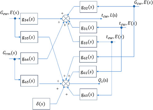
Figure 2. Open loop Chiller 2-inputs 2-outputs block diagram.

As $G_{rm}\left(t\right)$ and $G_{ew},E\left(t\right)$ are the main system manipulated inputs, the other inputs like $t_{cw},E$ and $t_{ew},E$ can be considered as additional disturbances that might affect both selected system outputs. $G_{cw},E$ can be held constant with a value of $1.16k\mathrm{g}·s^{-1}$ as a permanent input condition.

3 Results

This section evaluates the performance and significance of the derived open-loop chiller system model. Particular emphasis will be placed on the model’s behavior in response to perturbations in system inputs within the open-loop configuration and under various operational condition changes.

3.1 Importance of the developed 2-inputs 2-outputs open-loop model

The simplified mathematical model of the air conditioning chiller system, as shown in Equation 31, is crucial for engineers to develop control strategies in future studies that enhance system performance. As an open-loop model, it provides a straightforward view of the system’s behaviour without feedback effects. This foundational stage helps engineers understand how the system functions under various conditions and clarifies the relationship between inputs and outputs. With this understanding, they can design sophisticated control systems that aim to improve efficiency and overall performance.

Open-loop system responses are advantageous as they provide direct insights into the system’s behaviour, thereby facilitating the identification of inputs-such as refrigerant or coolant flow rates-that influence outputs like outlet temperature or cooling capacity. This model also helps pinpoint the key outputs that require monitoring and control. After understanding these aspects through open-loop modeling, engineers can design more sophisticated feedback control strategies to ensure the system runs efficiently and meets performance targets. Overall, the open-loop model serves as a strong foundation for developing responsive systems that optimise efficiency and boost performance.

3.2 Open loop responses

Open-loop responses involve analysing how the chiller’s outputs (e.g., outlet temperature and cooling capacity) react to changes in its inputs (e.g., flow rates) without any feedback control adjustments. This analysis helps in understanding the system’s natural dynamics, allowing engineers to design and optimise feedback controllers for better output regulation.

The block diagram described in Figure 2 was constructed using SIMULINK software, so when the open loop configuration is simulated with the initial conditions, including ($t_{cw},E=29.5℃$; $G_{cw},E=1.16kg/s$; $t_{ew},E=24.8℃$; $G_{ew},E=1.45kg/s,$; $G_{rm}=0.116kg/s$), the output responses were as illustrated in Figure 3. Based on the initial conditions of input values, the first configured chiller output $t_{ew},E\left(t\right)$ is approaching a steady state value of $21℃$ coupled with the second output $Q_c\left(t\right)$ approaching almost $1.02kW$.

Figure 3

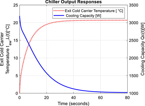
Figure 3. Open loop responses when applying initial conditions, including ($t_{cw},E\left(t\right)=29.5℃$; $G_{cw},E\left(t\right)=1.16kg/s$; $t_{ew},E\left(t\right)=24.8℃$; $G_{ew},E\left(t\right)=1.45kg/s,$; $G_{rm}\left(t\right)=0.116kg/s$).

It is worth mentioning that Figure 3 will be the benchmark for analysing the performance of the system under perturbations from other inputs.

For different operational conditions, the system behaviour under alterations in system inputs can also be captured and illustrated using SIMULINK. Figure 4 shows the system behaviour when cold carrier mass flow rate (first input, $G_{ew},E\left(t\right)$) is a step increase to $1.95kg/\mathit{sec}$, while the other inputs remain unchanged and adhere to their initial conditions. It can be noticed that there is a decrease in the exit cold carrier temperature $t_{ew},L\left(t\right)$ from $24.8℃$ to $22.8℃$ which is caused by the increase of $G_{ew},E\left(t\right)$ to $1.95kg/\mathit{sec}$.

Figure 4

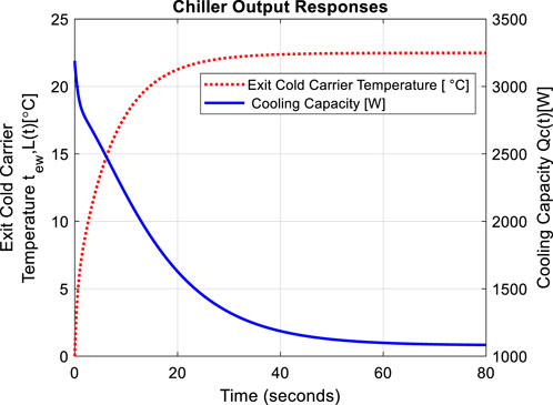
Figure 4. Open loop responses when applying step change in $G_{ew,}E\left(t\right)=1.95kg/s$ while other inputs remain unchanged as per initial conditions values.

For a different case, when the refrigerant mass flow rate (second input, $G_{rm}\left(t\right)$) is a step increase to $0.216kg/\mathit{sec}$, the resulting output responses are shown in Figure 5. Consequently, the exit cold carrier temperature $t_{ew},L\left(t\right)$ is decreasing to approximately 17.3 $℃$ with the coupling effect on the cooling capacity output increases to $2.35kW$

Figure 5

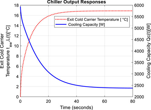
Figure 5. Open-loop responses when the refrigerant mass flow rate is increased to $G_{rm}\left(t\right)=0.216$ $kg/\mathit{sec}$ while other inputs remain unchanged as per the initial conditions values.

For a case where a step disturbance input on inlet temperature of the condenser coolant $t_{cw},E\left(t\right)$ is increasing to $40℃$ while all other inputs remain equal to their initial conditions, the output responses are depicted in Figure 6.

Figure 6

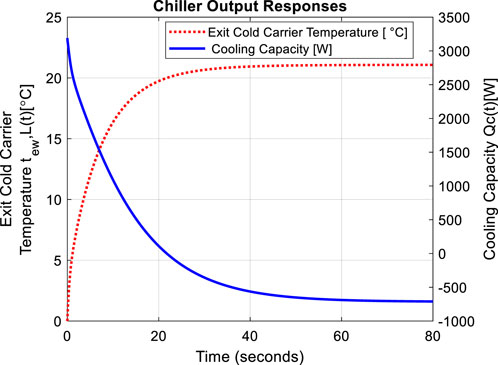
Figure 6. Open loop responses when applying step increase at $t_{cw},E\left(t\right)$ equal to 40$℃$ while other inputs remain unchanged and as per initial conditions.

Based on the initial conditions of other inputs, the exit cold carrier temperature $t_{ew},E\left(t\right)$ is approaching $21.5℃$ while the cooling capacity is approaching $-0.75kW$.

In a situation where a step disturbance input on the inlet temperature of the cold carrier fluid increases while all other inputs remain at their initial conditions, the output responses are shown in Figure 7. Based on the initial conditions of other inputs, the exit cold carrier temperature $t_{ew},E\left(t\right)$ is approaching $32.5℃$ while the cooling capacity is approaching $2.25kW$ associated with some oscillations.

Figure 7

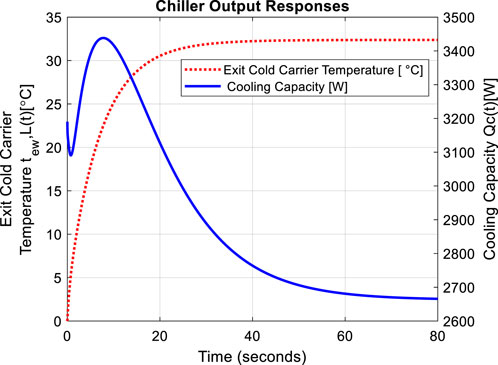
Figure 7. Open loop responses when applying step increase at $t_{ew},E\left(t\right)$ equal to 40$℃$ while other inputs remain unchanged.

The last case that will be discussed is when the disturbance step of $\delta \left(t\right)=-500W$ is applied due to dirt, scaling or foul in the evaporator while other inputs remain unchanged and as per their initial condition values. The results are illustrated in Figure 8. The responses show that no significant change in the exit cold carrier temperature ending with steady state value of $t_{ew,}L\left(t\right)=21℃$ and the cooling capacity is approaching steady state value of $Q_c\left(t\right)=0.55kW$.

Figure 8

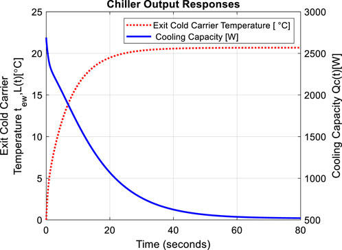
Figure 8. Open loop responses when applying step disturbance at $\delta \left(t\right)$ equal $-500W$ while other inputs remain unchanged.

4 Discussions

This section provides comprehensive interpretations of the system responses illustrated in Figures 3–8, to explain the system’s behaviour within the open-loop configuration. These insights aim to augment the understanding of system engineers, thereby facilitating the proposal of suitable control strategies.

In Figure 3 where the system is subjected to initial conditions which are basically ($t_{cw},E=29.5℃$; $G_{cw},E=1.16kg/s$; $t_{ew},E=24.8℃$; $G_{ew},E=1.45kg/s,$; $G_{rm}=0.116kg/s$), the first chiller output $t_{ew},E\left(t\right)$ is approaching a steady state value of $21℃$ coupled with the second output $Q_c\left(t\right)$ approaching almost $1.02kW$.

The decrease in $t_{ew},L\left(t\right)$ temperature from $24.8℃$ to $21℃$ indicates that the evaporator is successfully absorbing heat from the cold carrier fluid, causing its temperature to drop. This temperature reduction is typical of an evaporator’s operation, where heat from the fluid is transferred to the refrigerant, cooling the cold carrier fluid as it passes through. The system reaches a stable cooling output, meaning that the heat transfer in the evaporator has balanced out with the conditions imposed by the inputs (e.g., refrigerant flow rate $G_{rm}\left(t\right)$). The cooling capacity of $1.02kW$ reflects the rate at which the chiller removes heat from the cold carrier fluid. This steady-state value indicates that the system has reached an equilibrium where the refrigerant is effectively absorbing heat from the cold carrier fluid at a rate of $1.02kW$. The cooling capacity value shows that the chiller is operating at a relatively low load, typical for initial conditions with moderate refrigerant flow rates. As the cooling demand increases or the system parameters change (e.g., $G_{ew},E\left(t\right)$, $Q_c\left(t\right)$ would adjust accordingly.

Figure 3 will be the benchmark for analysing the performance of the system under perturbations from other inputs.

Figure 4 shows the system behaviour when cold carrier mass flow rate (first input, $G_{ew},E\left(t\right)$) is a step increase to $1.95kg/\mathit{sec}$, while the other inputs remain unaltered and as per their initial conditions. The decrease in exit cold carrier temperature $t_{ew},L\left(t\right)$ from $24.8℃$ to $22.8℃$ is caused by the increase of $G_{ew},E\left(t\right)$ to $1.95\text{\hspace{0.17em}kg}/\sec$. The difference is less than the previous case, when it was from $24.8℃$ to $20.8℃$. As more fluid is passing through the evaporator, the same amount of released heat is spread across a larger mass of fluid. This means that the cold carrier fluid releases less heat per unit of mass, causing a slower temperature reduction in the cold carrier as it moves through the evaporator. In the same time, as more fluid is passing through the evaporator, the same amount of released heat is spread across a larger mass of fluid so the cooling capacity ${\mathrm{Q}}_{\mathrm{c}}\left(\mathrm{t}\right)$ increases to approximately $1.15kW$, up from the previous steady-state value of $1.02\text{kW}$. The increase in $G_{ew,}E\left(t\right)$ does not only affect $t_{ew},L\left(t\right)$, but also impacts $Q_c\left(t\right)$, demonstrating an inherent coupling between these two outputs.

In Figure 5 when the refrigerant mass flow rate (second input, $G_{rm}\left(t\right)$) is a step increase to $0.216kg/\mathit{sec}$ the exit cold carrier temperature $t_{ew},L\left(t\right)$ is decreasing to approximately 17.3 $℃$ with coupling effect on the cooling capacity output increasing to $2.35\text{\hspace{0.17em}kW}$. By increasing $G_{rm}\left(t\right)$, the amount of refrigerant flowing through the evaporator increases. This allows the evaporator to absorb more heat from the cold carrier fluid (chilled water) causing a larger reduction in the temperature of the cold carrier fluid as it passes through the evaporator. The cooling capacity $Q_c\left(t\right)$ increases to 2.35 kW, up from the previous value of approximately 1.02 kW. The greater refrigerant flow rate allows the system to absorb more heat, which directly translates into a higher $Q_c\left(t\right)$ (cooling capacity). The system is now removing heat from the cold carrier at a higher rate to maintain the desired temperature decrease.

Similarly, in Figure 6, a step disturbance input on the inlet temperature of the condenser coolant $t_{cw},E\left(t\right)$ is increasing to $40℃$ while all other inputs remain equal to their initial conditions, the exit cold carrier temperature $t_{ew},E\left(t\right)$ is approaching $21.5℃$ while the cooling capacity is approaching $-0.75\text{\hspace{0.17em}kW}$. The increase in $t_{cw},E\left(t\right)$ (inlet coolant temperature to the condenser) reduces the condenser’s ability to reject heat. This results in higher refrigerant pressures and temperatures within the system, leading to a less effective heat exchange process in the evaporator. The temperature $t_{ew},L\left(t\right)$ rises to $21.5°C$, up from its previous steady-state value of $21°C$. With the evaporator unable to effectively absorb heat from the cold carrier fluid, the outlet temperature of the cold carrier fluid $t_{ew},L\left(t\right)$ increases slightly, reflecting a reduced cooling effect. A negative ${\mathrm{Q}}_{\mathrm{c}}\left(\mathrm{t}\right)$ indicates that instead of removing heat from the cold carrier, the chiller system is now adding heat. This happens because the condenser cannot reject enough heat due to the elevated ${\mathrm{t}}_{\text{cw}},\mathrm{E}\left(\mathrm{t}\right)$, causing a thermal imbalance in the refrigerant cycle. With the refrigerant unable to condense efficiently in the condenser, the evaporator’s cooling capacity is severely compromised, leading to the system effectively transferring heat into the cold carrier rather than removing it.

In Figure 7, the exit cold carrier temperature $t_{ew},E\left(t\right)$ is approaching $32.5℃$ while the cooling capacity is approaching $2.25kW$ associated with some oscillations. The increase in the inlet cold carrier temperature $t_{ew},E\left(t\right)$ to $40℃$ imposes a significantly higher thermal load on the evaporator, which can be understood as social housing occupancy dynamics. In high-density residential environments, such as social housing in extreme climates, occupant density and intermittent usage patterns can cause significant fluctuations in thermal loads. The 40°C disturbance models scenarios like peak occupancy or severe weather events, where internal heat gains increase due to higher occupant activity. As a result, the evaporator absorbs more heat from the cold carrier fluid, but it cannot reduce the temperature as effectively due to the larger thermal input. The exit temperature $t_{ew},L\left(t\right)$ stabilizes at $32.5℃$, reflecting the system’s new equilibrium under the higher inlet temperature. The increase in $t_{ew},E\left(t\right)$ raises the amount of heat the evaporator needs to absorb to maintain the cold carrier’s flow temperature. This causes the cooling capacity $Q_C\left(t\right)$ to increase significantly, as the evaporator works harder to remove the additional heat from the cold carrier fluid. The increase to $2.67\text{\hspace{0.17em}kW}$ reflects the system’s response to handle the higher thermal load introduced by the elevated inlet temperature.

The cooling capacity exhibits oscillations before reaching its steady-state value of $2.67\text{\hspace{0.17em}kW}$. The evaporator’s thermal response is dynamic, and a sudden increase in ${\mathrm{t}}_{\text{ew}},\mathrm{E}\left(\mathrm{t}\right)$ creates an imbalance in the heat transfer process. This imbalance induces transient oscillations as the system attempts to reach a new equilibrium. Any overshoot in heat absorption by the evaporator leads to fluctuations in cooling capacity before stabilization. The chiller system’s physical components, such as the refrigerant cycle and heat exchanger, exhibit thermal and fluidic inertia. These inertial effects delay the system’s ability to settle immediately after the disturbance, resulting in oscillatory behavior. As $t_{ew},E\left(t\right)$ increases, the heat absorbed by the evaporator rises, leading to simultaneous increases in $t_{ew},L\left(t\right)$ and $Q_C\left(t\right)$. This coupling is inherent in the chiller system’s design and reflects the interconnected nature of its heat transfer processes.

The results illustrated in Figure 8 due to disturbance applied on the system output show that no significant change in the exit cold carrier temperature ending with steady state value of $t_{ew,}L\left(t\right)=21℃$ but the cooling capacity is approaching steady state value of $Q_c\left(t\right)=0.55kW$. Despite the disturbance, the cold carrier fluid’s exit temperature is unaffected, reducing the chilled water temperature from $24.8℃$ to $21℃$. This indicates that the evaporator, though partially fouled, still manages to absorb sufficient heat to maintain the temperature difference required to cool the cold carrier fluid to $21℃$. The absence of a significant temperature change could result from the reduced heat transfer being compensated by the evaporator’s thermal inertia or by the refrigerant still operating within its effective range despite the fouling. On the other hand, the fouling in the evaporator reduces its ability to transfer heat effectively, directly decreasing the cooling capacity. A reduction of $500\mathrm{W}$ corresponds to the disturbance magnitude, which accounts for the drop in $Q_c\left(t\right)$ to $0.55kW$. This highlights the evaporator’s sensitivity to fouling and its direct impact on the system’s overall cooling performance. The reduced cooling capacity reflects a loss of energy efficiency, as the chiller is no longer operating at its full potential due to fouling. This could lead to higher operational costs and reduced performance in meeting cooling demands. This situation represents fouling or scaling in the evaporator, a common issue in social housing due to limited maintenance budgets and ageing infrastructure. Fouling reduces heat transfer efficiency, as evidenced by the drop in cooling capacity $Q_c\left(t\right)$ to $0.55kW$ without affecting outlet temperature $t_{ew,}L\left(t\right)$. This scenario underscores the importance of low-maintenance design and robust control in social housing, where infrequent servicing can degrade system performance. By quantifying fouling’s impact, the model supports the development of predictive maintenance strategies or fault-tolerant controls, critical for cost-sensitive and resource-constrained environments.

The open-loop simulation results of the simplified mathematical model provide valuable insights into the dynamic behavior of the chiller system, highlighting its sensitivity to input changes and disturbances. The results show how variables like $t_{ew},L\left(t\right)$ and $Q_c\left(t\right)$ respond passively, with phenomena such as coupling effects and oscillations, underscoring the system’s inability to maintain stability in some cases without feedback control. These findings emphasize the need for robust feedback control mechanisms to counteract disturbances, decouple interdependent outputs, and stabilize the system under varying conditions. Engineers can use this data along with the transfer function matrix in Equation 31 to design controllers, refine operational limits, and develop advanced strategies such as multivariable control techniques to enhance stability, reduce oscillations, and improve overall efficiency. By understanding these open-loop characteristics, system engineers are better equipped to optimize the chiller’s functionality and ensure reliable performance in real-world applications. The findings also highlight opportunities to integrate this model into sustainable social housing developments in the extreme climates areas, where adaptive HVAC systems can enhance energy resilience and occupant comfort.

5 Conclusion

This study presents a simplified multivariable state-space model of a vapor compression chiller system, emphasising the operation of key components such as the condenser and evaporator. The model expands upon an existing state-space mathematical framework, as detailed in (Yao et al., 2013), which has been validated through experimental data obtained from a chiller unit. While the original model in (Yao et al., 2013) involves a 5 × 7 multivariable structure with high-order dynamics, the current 2 × 2 model retains core thermal interactions while significantly reducing the state-space dimension, simplifying real-time control implementation. It delivers an accurate yet computationally straightforward mathematical model representation of the system’s behaviour. In control engineering, the mathematical model, represented through a state-space model, can be converted into a transfer function. The MIMO-related transfer function matrix plays a crucial role in the analysis of multivariable systems and controller design. It enables direct frequency-domain evaluation of input-output dynamics, such as system gain, phase lag, and coupling effects. For HVAC applications, especially vapor compression chillers, such a matrix is essential for designing decoupled or coordinated control strategies that regulate thermal outputs efficiently. The HVAC simplified mathematical model’s performance developed in this study is tested across different input scenarios using SIMULINK/MATLAB. The results are then plotted to validate the model’s ability to predict system responses. This includes scenarios such as operational changes, fouling, and thermal load variations. The open-loop simulation results demonstrate that the system reaches steady-state values after a certain response time, but the performance reveals significant interdependencies between outputs. For instance, the cooling capacity stabilizes at 1.02 kW, while the exit cold carrier temperature approaches 20.8°C under initial conditions, reflecting the system’s ability to reach equilibrium. The system reaches steady-state conditions in approximately 40 s for the exit cold carrier temperature and 70 s for the cooling capacity under nominal operating conditions. However, the simulation reveals strong input-output coupling, where a change in one input such as an increase in refrigerant mass flow rate affects both outputs simultaneously. For instance, a step increase in refrigerant flow from 0.116 kg/m3 to 0.216 kg/m3 not only lowers the cold carrier temperature to 17°C but also increases cooling capacity to 2.4 kW. Additionally, when subjected to a step disturbance in the condenser inlet temperature, the system exhibits oscillations in cooling capacity with a peak deviation of ±0.4 kW and a settling time exceeding 80 s. These dynamics highlight the system’s sensitivity to thermal and hydraulic disturbances, which would necessitate a multivariable control strategy that manages the system’s behaviour, aiming to enhance its performance while optimising its energy consumption. Therefore, implementing closed-loop multivariable control is essential. Such strategies can compensate for cross-coupling, dampen oscillations, and stabilize output responses in the presence of real-world disturbances and load variations, ensuring both performance and energy efficiency.

The novelty of this research lies in introducing a reduced-order multivariable model that retains essential dynamics while significantly lowering computational demands, making it suitable for cost-sensitive control applications. The simplified mathematical model can serve as the foundation for advanced feedback control designs that stabilise HVAC operation, decouple interacting outputs, and enhance energy efficiency, helping buildings meet sustainability targets without compromising comfort or reliability.

Future work could enhance the model’s accuracy by incorporating a secondary verification step to increase confidence. Since the model has been deemed accurate at the initial confidence level validated earlier with the Air Conditioning Experimental unit, future efforts might involve checking the simplified model’s accuracy at an additional confidence level. This can be achieved by testing the simplified mathematical model against a comparable experimental Air Conditioning unit, built based on the key parameters and components used in the model.

Data availability statement

The original contributions presented in the study are included in the article/supplementary material, further inquiries can be directed to the corresponding author.

Author contributions

BT: Writing – original draft, Investigation, Conceptualization, Software. MS: Resources, Supervision, Writing – review and editing, Project administration.

Funding

The author(s) declare that financial support was received for the research and/or publication of this article. The author would like to recognize the support provided by Ajman University and the Healthy and Sustainable Built Environment Research Center for the publication of this research.

Conflict of interest

The authors declare that the research was conducted in the absence of any commercial or financial relationships that could be construed as a potential conflict of interest.

Generative AI statement

The author(s) declare that Generative AI was used in the creation of this manuscript. The entire content is developed solely by the authors. Generative AI is used to improve the language and readability of the manuscript.

Publisher’s note

All claims expressed in this article are solely those of the authors and do not necessarily represent those of their affiliated organizations, or those of the publisher, the editors and the reviewers. Any product that may be evaluated in this article, or claim that may be made by its manufacturer, is not guaranteed or endorsed by the publisher.

References

Abdo-Allah, A., Iqbal, T., and Pope, K. (2017). “Modeling and analysis of an HVAC system for the S.J. carew building at memorial university,” in Canadian Conference on Electrical and Computer Engineering, Windsor, ON, Canada, 30 April 2017 - 03 May 2017 (IEEE). doi:10.1109/CCECE.2017.7946689

CrossRef Full Text | Google Scholar

Abdo-Allah, A., Iqbal, T., and Pope, K. (2018). Modeling, analysis, and state feedback control design of a multizone HVAC system. J. Energy 2018, 1–11. doi:10.1155/2018/4303580

CrossRef Full Text | Google Scholar

Addis, B. (2020). Past, current and future use of physical models in civil engineering design. Proc. Institution Civ. Eng. Civ. Eng. 174 (2), 61–70. doi:10.1680/jcien.20.00028

CrossRef Full Text | Google Scholar

Afram, A., and Janabi-Sharifi, F. (2014). Review of modeling methods for HVAC systems. Appl. Therm. Eng. 67, 507–519. doi:10.1016/j.applthermaleng.2014.03.055

CrossRef Full Text | Google Scholar

Ali, M. (2019). Developing a white-box modelling of residential air conditioning based on demand response algorithm. J. Build. Eng. doi:10.13140/RG.2.2.26588.13445

CrossRef Full Text | Google Scholar

Angel, W. L. (2011). HVAC design sourcebook. New York, NY, USA: McGraw Hill Professional.

Google Scholar

Asim, N., Badiei, M., Mohammad, M., Razali, H., Rajabi, A., Chin Haw, L., et al. (2022). Sustainability of heating, ventilation and air-conditioning (HVAC) systems in buildings—an overview. Int. J. Environ. Res. Public Health 19 (2), 1016. doi:10.3390/ijerph19021016

PubMed Abstract | CrossRef Full Text | Google Scholar

Bacher, P., and Madsen, H. (2011). Identifying suitable models for the heat dynamics of buildings. Energy Build. 43 (7), 1511–1522. doi:10.1016/j.enbuild.2011.02.005

CrossRef Full Text | Google Scholar

Castleton, H. F., Stovin, V., Beck, S. B. M., and Davison, J. B. (2010). Green roofs; building energy savings and the potential for retrofit. Energy Build. 42 (10), 1582–1591. doi:10.1016/j.enbuild.2010.05.004

CrossRef Full Text | Google Scholar

Goetzler, W., Guernsey, M., Young, J., Fuhrman, J., and Abdelaziz, O. (2016). The future of air conditioning for buildings. Available online at: www.osti.gov/home/.

Google Scholar

Hassan, M. R., and Al-Samarraie, S. A. (2022). Robust nonlinear control design for the HVAC system based on adaptive sliding mode control. J. Eur. Des Systèmes Automatisés 55 (5), 593–601. doi:10.18280/jesa.550504

CrossRef Full Text | Google Scholar

Homod, R. Z. (2013). Review on the HVAC system modeling types and the shortcomings of their application. J. Energy 2013, 1–10. doi:10.1155/2013/768632

CrossRef Full Text | Google Scholar

Jang, H., Kang, B., Cho, K., Jang, K., and Park, S. (2019). Design and implementation of IoT-based HVAC and lighting system for energy saving. MATEC Web Conf. 260, 02012. doi:10.1051/matecconf/201926002012

CrossRef Full Text | Google Scholar

Jin, G. Y., Tan, P. Y., Ding, X. D., and Koh, T. M. (2011). “Cooling coil unit dynamic control of in HVAC system,” in Proceedings of the 2011 6th IEEE Conference on Industrial Electronics and Applications, ICIEA 2011, Beijing, China, 21-23 June 2011 (IEEE), 942–947. doi:10.1109/ICIEA.2011.5975722

CrossRef Full Text | Google Scholar

Jorissen, F., Picard, D., Six, K., and Helsen, L. (2021). Detailed white-box non-linear model predictive control for scalable building HVAC control. Proceedings of 14th Modelica Conference 2021. Linköping, Sweden, September 20-24, 2021, 315–323. doi:10.3384/ecp21181315

CrossRef Full Text | Google Scholar

Kathiravel, R., Zhu, S., and Feng, H. (2024). LCA of net-zero energy residential buildings with different HVAC systems across Canadian climates: a BIM-Based fuzzy approach. Energy Build. 306, 113905. doi:10.1016/J.ENBUILD.2024.113905

CrossRef Full Text | Google Scholar

Lapinskiene, V., and Martinaitis, V. (2013). The framework of an optimization model for building envelope. Procedia Eng. 57, 670–677. doi:10.1016/j.proeng.2013.04.085

CrossRef Full Text | Google Scholar

Li, J., Poulton, G., Platt, G., Wall, J., and James, G. (2010). Dynamic zone modelling for HVAC system control. Int. J. Model. Identif. Control 9 (1–2), 5–14. doi:10.1504/IJMIC.2010.032354

CrossRef Full Text | Google Scholar

Li, P., Qiao, H., Li, Y., Seem, J. E., Winkler, J., and Li, X. (2014). Recent advances in dynamic modeling of HVAC equipment. Part 1: equipment modeling. HVAC R Res. 20 (1), 136–149. doi:10.1080/10789669.2013.836877

CrossRef Full Text | Google Scholar

Li, Y., Karunathilake, D., Vilathgamuwa, D. M., Mishra, Y., Farrell, T. W., Choi, S. S., et al. (2022). Model order reduction techniques for physics-based lithium-ion battery management: a survey. IEEE Ind. Electron. Mag. 16 (3), 36–51. doi:10.1109/MIE.2021.3100318

CrossRef Full Text | Google Scholar

Ma, Y., Matusko, J., and Borrelli, F. (2015). Stochastic model predictive control for building HVAC systems: complexity and conservatism. IEEE Trans. Control Syst. Technol. 23 (1), 101–116. doi:10.1109/TCST.2014.2313736

CrossRef Full Text | Google Scholar

Ma, Z., Cooper, P., Daly, D., and Ledo, L. (2012). Existing building retrofits: methodology and state-of-the-art. Energy Build. 55, 889–902. doi:10.1016/j.enbuild.2012.08.018

CrossRef Full Text | Google Scholar

Murphy, M. D., O’sullivan, P. D., da Graça, G. C., and O’donovan, A. (2021). Development, calibration and validation of an internal air temperature model for a naturally ventilated nearly zero energy building: Comparison of model types and calibration methods. Energies 14 (4), 871. doi:10.3390/en14040871

CrossRef Full Text | Google Scholar

Palmero-marrero, A. I., and Oliveira, A. C. (2010). Effect of louver shading devices on building energy requirements. Appl. Energy 87 (6), 2040–2049. doi:10.1016/j.apenergy.2009.11.020

CrossRef Full Text | Google Scholar

Pan, Y., Zhu, M., Lv, Y., Yang, Y., Liang, Y., Yin, R., et al. (2023). Building energy simulation and its application for building performance optimization: a review of methods, tools, and case studies. Adv. Appl. Energy 10, 100135. doi:10.1016/J.ADAPEN.2023.100135

CrossRef Full Text | Google Scholar

Pavlak, G. S., Florita, A. R., Henze, G. P., and Rajagopalan, B. (2014). Comparison of traditional and Bayesian calibration techniques for gray-box modeling. J. Archit. Eng. 20 (2). doi:10.1061/(asce)ae.1943-5568.0000145

CrossRef Full Text | Google Scholar

Seyam, S. (2018). Types of HVAC systems. HVAC Syst. doi:10.5772/intechopen.78942

CrossRef Full Text | Google Scholar

Silvestri, A., Lydon, G., Waibel, C., Wu, D., Schlueter, A., Silvestri, A., et al. (2023). Data-driven reduced order modelling using clusters of thermal dynamics conference paper data-driven reduced order modelling using clusters of thermal dynamics. Build. Simul. Conf. Proc. 18. doi:10.3929/ethz-b-000634990

CrossRef Full Text | Google Scholar

Simpeh, E. K., Pillay, J. P. G., Ndihokubwayo, R., and Nalumu, D. J. (2022). Improving energy efficiency of HVAC systems in buildings: a review of best practices. Int. J. Build. Pathology Adapt. 40 (2), 165–182. doi:10.1108/IJBPA-02-2021-0019

CrossRef Full Text | Google Scholar

Subbaram Naidu, D., and Rieger, C. G. (2011). Advanced control strategies for heating, ventilation, air-conditioning, and refrigeration systems - an overview: part I: hard control. HVAC R Res. 17 (1), 2–21. doi:10.1080/10789669.2011.540942

CrossRef Full Text | Google Scholar

Touqan, B., Abdul-Ameer, A., and Salameh, M. (2022). HVAC multivariable system modelling and control. Proc. Institution Mech. Eng. Part C J. Mech. Eng. Sci. 237, 2049–2061. doi:10.1177/09544062221138836

CrossRef Full Text | Google Scholar

Touqan, B., and Ameer, A. A. (2024). Enhancing HVAC multivariable system performance through hybrid modeling and direct nyquist array control. Build. Serv. Eng. Res. Technol. 45, 833–861. doi:10.1177/01436244241274107

CrossRef Full Text | Google Scholar

Touqan, B., Taleb, H., and Salameh, M. (2017). Low carbon cooling approach for the residences in the UAE: a case study in Dubai. World Congr. Civ. Struct. Environ. Eng. doi:10.11159/awspt17.127

CrossRef Full Text | Google Scholar

Whalley, R., and Abdul-Ameer, A. (2011). Heating, ventilation and air conditioning system modelling. Build. Environ. 46 (3), 643–656. doi:10.1016/j.buildenv.2010.09.010

CrossRef Full Text | Google Scholar

Wu, Y., and Xue, W. (2024). Data-driven weather forecasting and climate modeling from the perspective of development. Multidiscip. Digit. Publ. Inst. (MDPI) 15 (Issue 6), 689. doi:10.3390/atmos15060689

CrossRef Full Text | Google Scholar

Yao, Y., Huang, M., and Chen, J. (2013). State-space model for dynamic behavior of vapor compression liquid chiller. Int. J. Refrig. 36 (8), 2128–2147. doi:10.1016/j.ijrefrig.2013.05.006

CrossRef Full Text | Google Scholar

Zhang, L. (2023). Challenges and opportunities of machine learning control in building operations. Springer Nature Link.

Google Scholar

Zhao, J., Li, X., Shum, C., and McPhee, J. (2021). A review of physics-based and data-driven models for real-time control of polymer electrolyte membrane fuel cells. Energy AI 6, 100114. doi:10.1016/J.EGYAI.2021.100114

CrossRef Full Text | Google Scholar

Zhou, D., Hu, Q., and Tomlin, C. J. (2016). Model comparison of a data-driven and a physical model for simulating HVAC systems. Available online at: http://arxiv.org/abs/1603.05951.

Google Scholar

Zhou, D. P., Hu, Q., and Tomlin, C. J. (2017). Quantitative comparison of data-driven and physics-based models for commercial building HVAC systems. Proceedings of the American Control Conference, 2900–2906. Seattle, WA, USA 24-26 May 2017. doi:10.23919/ACC.2017.7963391

CrossRef Full Text | Google Scholar

Zlatanović, I., Gligorević, K., Ivanović, S., and Rudonja, N. (2011). Energy-saving estimation model for hypermarket HVAC systems applications. Energy Build. 43 (12), 3353–3359. doi:10.1016/j.enbuild.2011.08.035

CrossRef Full Text | Google Scholar

Glossary

Nomenclature

$t_{cw},E\left(t\right)$ Inlet coolant temperature of the condenser [$\left.℃\right]$

$t_{cw},L\left(t\right)$ Outlet coolant temperature of the condenser [$\left.℃\right]$

$G_{cw},E\left(t\right)$ Coolant flow rate into the condenser $\left[kg/s\right]$

$t_{ew},E$ (t) Inlet cold carrier temperature of the evaporator [$\left.℃\right]$

$t_{ew},L\left(t\right)$ Outlet cold carrier temperature of the evaporator [$\left.℃\right]$

$G_{ew},E\left(t\right)$ Cold carrier flow rate into the evaporator $\left[kg/s\right]$

$G_{rm}\left(\mathrm{t}\right)$ Refrigerant mass flow rate $\left[kg/s\right]$

$t_c\left(t\right)$ The temperature of the refrigerant at the outlet of the condenser, representing the condensing phase in the refrigeration cycle $\left[℃\right]$

$t_k\left(t\right)$ The temperature of the refrigerant at the inlet of the evaporator, representing the evaporating phase in the refrigeration cycle $\left[℃\right]$

$t_{cg}\left(t\right)$ The temperature of the shell wall of the condenser, representing the thermal condition of the condenser’s external surface $\left[℃\right]$

$t_{eg}\left(t\right)$ The temperature of the shell wall of the evaporator, representing the thermal condition of the evaporator’s external surface $\left[℃\right]$

$W_{w,com}\left(t\right)$ This represents the work done by the compressor in the refrigeration cycle $\left[W\right]$

$Q_c\left(t\right)$ Refers to the amount of heat rejected by the refrigerant in the condenser to the surroundings or a cooling medium (e.g., water or air) $\left[W\right]$

$COP\left(t\right)$ This is a dimensionless measure of the efficiency of the refrigeration system. It is defined as the ratio of the cooling effect to the work input

Abbreviations

AC Air Conditioning

HVAC Heating Ventilation, and Air Conditioning

MIMO Multiple Input, Multiple Output

SISO Single Input, Single Output

COP Coefficient of Performance COP measures chiller efficiency by comparing cooling output (kW) to energy input (kW).

FCU Fan Coil Unit

IEA International Energy Agency

OECD Organisation for Economic Co-operation and Development

ML Machine Learning

AI Artificial Intelligence

MATLAB Matrix Laboratory (Simulation Software)