Stochastic stratigraphic simulation using image warping from sparse data

Quantifying stratigraphic uncertainty is crucial for reliable risk assessment and informed decision-making in geotechnical and geological engineering. However, accurately modeling complex stratigraphy—especially in heterogeneous settings influenced by irregular deposition—remains a challenge, particularly with limited site data. This study introduces a novel solution, modeling stratigraphy as a categorical random field and using image warping to transform non-stationary random fields into stationary ones, facilitating fast and realistic stochastic simulation. The method demonstrates high accuracy and computational efficiency in capturing complex stratigraphic profiles with quantified uncertainty. Validation through synthetic and real-world cases confirms the approach’s reliability and applicability.

1 Introduction

Ensuring safety in the design and construction of underground structures and geosystems remains a major challenge, largely due to limited stratigraphic data (Wang et al., 2018). Inferring stratigraphic information and accurately quantifying its uncertainty are essential, as inherent stratigraphic variability greatly impacts the performance of geosystems (Zhang et al., 2022). Despite its importance, obtaining complete stratigraphic information at a site is practically unfeasible due to limitations in site exploration data (Shi and Wang, 2023). The lack of stratigraphic data increases the risk of incidents during construction due to unexpected geological conditions (Ioannou, 1988). Understanding stratigraphic uncertainty and its impact on the design and construction of geosystems remains a persistent challenge (Wang et al., 2018).

Quantifying stratigraphic uncertainty, particularly in 3D subsurface modeling, remains an emerging field. Various stochastic modeling frameworks address this challenge. For cone penetration testing (CPT) data, methods like CPT-based modeling using the Robertson chart (Robertson, 1990) and Bayesian compressive sampling (Wang and Zhao, 2017) show promise. For borehole log data, techniques such as coupled Markov chain (CMC) models (Qi et al., 2016; Zhang et al., 2022), and IC-XGBoost (Shi and Wang, 2023) are used. However, these methods have certain limitations. Classical CMC models, relying on vertical and horizontal transition probability matrices, may produce inaccurate soil profiles, requiring mitigation (Li et al., 2019). IC-XGBoost depend on training images tied to specific engineering contexts, posing challenges with limited prior data. Stochastic stratigraphic modeling continues to be a dynamic research area in geotechnical engineering and engineering geology.

Recent advancements in Markov random field (MRF)-based stochastic simulation offer a robust framework for capturing spatial constraints, effectively modeling the anisotropy and heterogeneity of stratigraphic formations (Wei and Wang, 2022). Consequently, MRF models have gained prominence in addressing stratigraphic uncertainty. However, existing implementations (Gong et al., 2020; Li et al., 2016; Wang et al., 2017) often face challenges, such as subjective parameter definition and unrealistic soil profile generation. While the innovative MRF model by Wei and Wang (2022) addresses some limitations, it struggles with non-stationary spatial heterogeneity, such as tectonically distorted or irregularly deposited strata.

This study introduces a novel approach integrating image warping with an advanced stochastic stratigraphic simulation model to address challenges in modeling non-stationary stratigraphic fields. The image warping technique, using thin plate splines, transforms complex non-stationary fields into stationary ones. An in-house stochastic model, combining the MRF approach with a discriminant adaptive nearest neighbor-based k-harmonic mean distance (DANN-KHMD) classifier (Wei and Wang, 2022) in a Bayesian framework, is then applied. This enhances stratigraphic uncertainty estimation from sparse borehole data, improving the robustness and accuracy of MRF-based methods. The approach excels in handling complex non-stationary stratigraphy with limited data, offering two key benefits: simplifying non-stationary fields into stationary ones and enabling unsupervised sampling and updating of stratigraphic configurations.

2 Methods

The proposed model consists of four components: a) Markov random field, b) Bayesian machine learning, c) unsupervised classifier, and d) image warping technique. In our previous work (Wei and Wang, 2022), a model for stationary fields was developed using components a), b), and c). In this work, new component d) is introduced and integrated, allowing the model to handle non-stationary categorical random fields.

2.1 Review of previous work

2.1.1 Markov random field

The domain of a two-dimensional stratigraphic profile can be discretized into pixels through a uniform square lattice. An undirected graph, derived from the lattice grid, can facilitate the construction of an MRF. The joint probability of soil types at all lattice grid points $P\left(\mathit{x}\right)$ can be expressed by Equation 1:

$P\left(\mathit{x}\right)=\frac{\exp \left(-U\left(\mathit{x}\right)/T\right)}{{\displaystyle {\sum }_{\mathit{x}\in \mathrm{\Omega }}}\exp \left(-U\left(\mathit{x}\right)/T\right)}(1)$

in which, $U\left(\mathit{x}\right)$ is the energy of the soil type configuration $\mathit{x}=\left\{x_i|i\in \mathbf{S},x_i\in \mathbf{L}\right\}$, in which $x_i$, $\mathbf{S}=\left\{1,2,3,...,s\right\}$ and $\mathbf{L}=\left\{1,2,3,...,l\right\}$ represent the grid points and all soil types, respectively. $\mathrm{\Omega }=\left\{\mathit{x}=\left\{x_i\right\}\left|i\in \mathbf{S},x_i\in \mathbf{L}\right.\right\}$ is a configuration space that contains all possible soil profiles. The symbol $T$ can be straightforwardly configured as a constant unit (Geman and Geman, 1984). Locally, the conditional probability can be expressed as the following Equation 2:

$P\left(x_i|{\mathit{x}}_{{\mathrm{\partial }}_i}\right)=\frac{P\left(x_i,{\mathit{x}}_{{\mathrm{\partial }}_i}\right)}{{\displaystyle {\sum }_{{x_i}^{\prime }\in L}}P\left({x_i}^{\prime },{\mathit{x}}_{{\mathrm{\partial }}_i}\right)}=\frac{\exp \left[-U\left(x_i,{\mathit{x}}_{{\mathrm{\partial }}_i}\right)\right]}{{\displaystyle {\sum }_{{x_i}^{\prime }\in L}}\exp \left[-U\left({x_i}^{\prime },{\mathit{x}}_{{\mathrm{\partial }}_i}\right)\right]}(2)$

where $U\left(x_i,{\mathit{x}}_{{\mathrm{\partial }}_i}\right)$ is the local energy of the local neighborhood system ${\mathrm{\partial }}_i$, and ${x_i}^{\prime }$ indicates any possible label at pixel $i$, which loops over L. The local energy $U\left(x_i,{\mathit{x}}_{{\mathrm{\partial }}_i}\right)$ is characterized by the Potts model using Equation 3 (Koller and Friedman, 2009):

$U\left(x_i,{\mathit{x}}_{{\mathrm{\partial }}_i}\right)=V_i\left(x_i\right)+{\displaystyle \sum _{j\in {\mathrm{\partial }}_i}}{V}_{i,j}\left(x_i,x_j\right)(3)$

Within this equation, $V_i\left(x_i\right)$ represents the potential function uniquely associated with pixel $i$. $V_{i,j}\left(x_i,x_j\right)$ measures the potential indicating the local contextual constraint between adjacent pixels using Equation 4:

$V_{i,j}\left(x_i,x_j\right)=\left\{\begin{array}{l}0\text{\hspace{0.5em}if\hspace{0.5em}}{x}_i=x_j\\ {\beta }_d\text{\hspace{0.5em}if\hspace{0.5em}}{x}_i\ne x_j\end{array}\right.(4)$

Herein, ${\beta }_d\in \mathit{\beta }=\left\{{\beta }_1,{\beta }_2,{\beta }_3,{\beta }_4\right\}$ is granularity coefficient, indicating the contextual constraint in four independent directions.

2.1.2 Bayesian machine learning

All pixels in the modeling domain are categorized into two groups: a) pixels with known soil type indicating sparse borehole information ${\mathit{x}}_{BH}$, and b) pixels with unknown labels ${\mathit{x}}_{unknown}$ elsewhere. Both ${\mathit{x}}_{unknown}$ and $\mathit{\beta }$ need to be inferred given ${\mathit{x}}_{BH}$. A Markov Chain Monte Carlo (MCMC) technique is employed to sample ${\mathit{x}}_{unknown}$ and $\mathit{\beta }$ iteratively via two conditional posterior distributions $P\left({\mathit{x}}_{unknown}\left|{\mathit{x}}_{BH},\mathit{\beta }\right.\right)$ and $P\left(\mathit{\beta }\left|{\mathit{x}}_{unknown},{\mathit{x}}_{BH}\right.\right)$.

During the sampling process, the local energy at any pixel is calculated using Equation 3, based on the current label field. Equation 2 measures the likelihood for selecting each soil label at this pixel. Iterations of $P\left({\mathit{x}}_{unknown}\left|{\mathit{x}}_{BH},\mathit{\beta }\right.\right)$ are simulated using a parallel approach, designated as the chromatic sampler (Wang et al., 2017). Following updating ${\mathit{x}}_{unknown}$, $\mathit{\beta }$ can be derived from $P\left(\mathit{\beta }\left|{\mathit{x}}_{unknown},{\mathit{x}}_{BH}\right.\right)$ by Equation 5:

$\text{Post}\left(\mathit{\beta }\right)\propto \text{Prior}\left(\mathit{\beta }\right)L\left({\mathit{x}}_{unknown},{\mathit{x}}_{BH}|\mathit{\beta }\right)(5)$

where $\text{Post}\left(\mathit{\beta }\right)$ and $\text{Prior}\left(\mathit{\beta }\right)$ are posterior and prior distributions of $\mathit{\beta }$, respectively; $L\left({\mathit{x}}_{unknown},{\mathit{x}}_{BH}\left|\mathit{\beta }\right.\right)$ is the likelihood function of the simulated soil profile given $\mathit{\beta }$ as expressed by Equation 6:

$\begin{array}{ll}\hfill L\left({\mathit{x}}_{unknown},{\mathit{x}}_{BH}|\mathit{\beta }\right)=& {\displaystyle \prod _{x_i\in \left\{{\mathit{x}}_{unknown},{\mathit{x}}_{BH}\right\}}}P\left(x_i|{\mathit{x}}_{{\mathrm{\partial }}_i};\mathit{\beta }\right)\hfill \\ \hfill & ={\displaystyle \prod _{x_i\in \left\{{\mathit{x}}_{unknown},{\mathit{x}}_{BH}\right\}}}\frac{\exp \left[-U\left(x_i,{\mathit{x}}_{{\mathrm{\partial }}_i}\right)\right]}{{\displaystyle {\sum }_{{x_i}^{\prime }\in L}}\exp \left[-U\left({x_i}^{\prime },{\mathit{x}}_{{\mathrm{\partial }}_i}\right)\right]}\hfill \end{array}(6)$

$\text{Prior}\left(\mathit{\beta }\right)$ is modeled as a multivariate Gaussian distribution, encompasses a mean vector $\mathit{\mu }=\left[{\mu }_1,{\mu }_2,{\mu }_3,{\mu }_4\right]$ and a diagonal covariance matrix ${\sum }_{\beta }=diag\left({\sigma }_1^2,{\sigma }_2^2,{\sigma }_3^2,{\sigma }_4^2\right)$, where ${\mu }_i$ and ${\sigma }_i$ symbolize the preliminary estimates and standard deviation of the respective $\mathit{\beta }$. The Metropolis-Hastings (M-H) algorithm (Hastings, 1970) is employed to implement the MCMC sampling process for updating $\mathit{\beta }$.

2.1.3 DANN-KHMD classifier

The DANN-KHMD classifier is employed to initialize ${\mathit{x}}_{unknown}$. The spatial constraint metric ${\mathrm{\Psi }}_i$ at pixel i can be evaluated following the approach proposed by (Hastie and Tibshirani, 1996). Then, the DANN distance $D\left(j,i\right)$ between pixels $j$ and the center pixel $i$ can be calculated using the local metric ${\mathrm{\Psi }}_i$ as expressed by Equation 7:

$D\left(j,i\right)={\left({\mathit{v}}_j-{\mathit{v}}_i\right)}^{\mathbf{T}}{\mathrm{\Psi }}_i\left({\mathit{v}}_j-{\mathit{v}}_i\right)(7)$

Then, the harmonic mean distance (HMD) is calculated using the Equation 8 (Pan et al., 2017):

$HM{D}_i^{\left(m\right)}=\frac{k}{{\displaystyle {\sum }_{j=1}^k}\frac{1}{D\left(j,i\right)}},x_j=m(8)$

The HMD is then integrated into the local energy $U\left(x_i,{\mathit{x}}_{{\mathrm{\partial }}_i}\right)=HM{D}_i^{\left(x_i\right)}+{\displaystyle \sum _{j\in {\mathrm{\partial }}_i}}{V}_{i,j}\left(x_i,x_j\right)$ and the conditional probability Equation 2 for a local neighborhood system is updated as Equation 9:

$P\left(x_i|{\mathit{x}}_{{\mathrm{\partial }}_i}\right)=\frac{\exp \left[-\left(HM{D}_i^{\left(x_i\right)}+{\displaystyle {\sum }_{j\in {\mathrm{\partial }}_i}}{V}_{i,j}\left(x_i,x_j\right)\right)\right]}{{\displaystyle {\sum }_{{x_i}^{\prime }\in \mathbf{L}}}\exp \left[-\left(HM{D}_i^{\left({x_i}^{\prime }\right)}+{\displaystyle {\sum }_{j\in {\mathrm{\partial }}_i}}{V}_{i,j}\left({x_i}^{\prime },x_j\right)\right)\right]}(9)$

More details about Markov random field, Bayesian machine learning and DANN-KHMD classifier are shown in the authors’ previous work (Wei and Wang, 2022).

2.2 Image warping technique

2.2.1 Thin plate spline warping algorithm

This section delineates the methodology for implementing the image warping technique in the context of stratigraphical modeling by leveraging a sparse array of control points, denoted as $\left({\overline{x}}_i,{\overline{y}}_i\right)$ and accompanied by their respective displacements, $\left(\Delta {\overline{x}}_i,\Delta {\overline{y}}_i\right)$. The objective is to derive a transformation mapping, $f:\left(\overline{x},\overline{y}\right)\to \left({\overline{x}}^{\prime },{\overline{y}}^{\prime }\right)$, which facilitates the transition of pixels from the initial image to those in the deformed or warped image. This ensures the warped control points, $\left({{\overline{x}}_i}^{\prime },{{\overline{y}}_i}^{\prime }\right)$, align closely with their intended targets, $\left({\overline{x}}_i+\Delta {\overline{x}}_i,{\overline{y}}_i+\Delta {\overline{y}}_i\right)$, while ensuring the deformation of adjacent points maintains maximal smoothness. Figure 1a,b illustrates this concept, where red crosses and blue dots represent the control points $\left({\overline{x}}_i,{\overline{y}}_i\right)$ and their corresponding target points $\left({\overline{x}}_i+\Delta {\overline{x}}_i,{\overline{y}}_i+\Delta {\overline{y}}_i\right)$, respectively, within the initial image framework. The subsequent goal is to ascertain a smooth function, capable of yielding discrete displacements along the X-direction and Y-direction, thereby facilitating a comprehensive and smooth mapping of all points from the initial to the warped image.

Figure 1

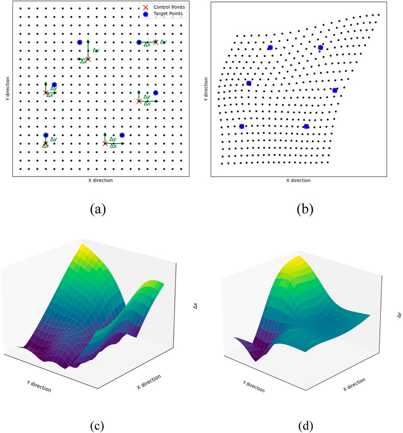
Figure 1. Illustrations for Thin Plate Spline warping algorithm. (a) Control points in initial image; (b) Control points in warped image; (c) Displacement surfaces in X direction; (d) Displacement surfaces in Y direction.

The Thin Plate Spline (TPS) warping algorithm is selected for addressing the two-dimensional image warping challenges, given its proficiency in facilitating smooth interpolation among a set of control points. TPS methodology interpolates a surface that seamlessly integrates each control point, implying that a triad of points would suffice to constitute a flat plane. Conceptually, the control points serve as positional constraints upon a flexible surface, where the optimal surface configuration is characterized by minimal bending. Illustratively, the $\Delta \overline{x}$ and $\Delta \overline{y}$ displacements between points $\left({{\overline{x}}_i}^{\prime },{{\overline{y}}_i}^{\prime }\right)$ and $\left({\overline{x}}_i,{\overline{y}}_i\right)$ can be visualized as the elevation of a three-dimensional smooth surface, which is mandatorily constrained to intersect all six control points, as depicted in Figures 1c,d.

This least bent surface is given by the following Equation 10 (i.e., the smooth function) (Bookstein, 1989; Donato and Belongie, 2003):

$f\left(\overline{x},\overline{y}\right)=a_1+a_{x}x+a_{y}y+{\displaystyle \sum _{i=1}^N}{\omega }_{i}dist\left(‖\left({\overline{x}}_i,{\overline{y}}_i\right)-\left(\overline{x},\overline{y}\right)‖\right)(10)$

in which the first three coefficients $\left(a_1,a_x,a_y\right)$ correspond to the linear part which defines a flat plane that best approximates all control points. The last term corresponds to the bending forces provided by N control points. There is a coefficient ${\omega }_i$ for each control point $i$, which denotes the weight of control point $i$ to the final displacement in X-direction or Y-direction. The smooth function gives us the warped points $\left({{\overline{x}}_i}^{\prime },{{\overline{y}}_i}^{\prime }\right)$ given origin grid points $\left({\overline{x}}_i,{\overline{y}}_i\right)$ in the initial image. The terms $‖\left({\overline{x}}_i,{\overline{y}}_i\right)-\left(\overline{x},\overline{y}\right)‖$ represents the distance from a control point $\left({\overline{x}}_i,{\overline{y}}_i\right)$ to a position $\left(\overline{x},\overline{y}\right)$. This distance is used in the function $dist\left(r\right)$ defined by Equation 11 (Bookstein, 1989; Donato and Belongie, 2003):

$dist\left(r\right)=r^2\log \left(r\right)(11)$

In addition to the smooth function Equation 10, we need additional constraints to the system following Bookstein (1989) and Donato and Belongie (2003):

${\displaystyle \sum _{i=1}^N}{\omega }_i=0(12)$

${\displaystyle \sum _{i=1}^N}{\omega }_i{\overline{x}}_i={\displaystyle \sum _{i=1}^N}{\omega }_i{\overline{y}}_i=0(13)$

Having Equations 10, 12 and 13, a linear system can be yielded for the TPS coefficients:

$\left[\begin{array}{cc}K& P\\ P^T& O\end{array}\right]\times \left[\begin{array}{l}\omega \\ a\end{array}\right]=\left[\begin{array}{l}v\\ o\end{array}\right](14)$

in which $O$ is a $3\times 3$ matrix of zeros, $o$ is a $3\times 1$ column vector of zeros. $\omega$ and $v$ are column vectors formed from ${\omega }_i$ and $v_i$, respectively, and $a$ is the column vector with elements $a_1$, $a_x$, $a_y$. The matrix $K$ evaluates the function $dist\left(r_{ij}\right)$ where $r_{ij}$ is the distance between two points $i$ and $j$. Matrix $K$ is expressed using Equation 15:

$K={\left[\begin{array}{ccc}dist\left(r_{11}\right)& dist\left(r_{12}\right)& ...\\ dist\left(r_{21}\right)& dist\left(r_{22}\right)& ...\\ ...& ...& dist\left(r_{nn}\right)\end{array}\right]}_{n\times n}(15)$

Matrix P contains the position information of all control points, as expressed by Equation 16:

$P={\left[\begin{array}{ccc}1& {\overline{x}}_1& {\overline{y}}_1\\ 1& {\overline{x}}_2& {\overline{y}}_2\\ ...& & \\ 1& {\overline{x}}_n& {\overline{y}}_n\end{array}\right]}_{3\times n}(16)$

Given a few control points and the corresponding warped control points (say target points), the matrices $K$, $P$ and vector $v$ are known since $K$ can be calculated only using control points. Therefore, the vector ${\left[\begin{array}{cc}\omega & a\end{array}\right]}^T$ containing the weight ${\omega }_i$ for each control point $i$ and coefficients $\left(a_1,a_x,a_y\right)$ can be solved according to Equation 14. As a result, the warped position of any point in the initial image can be computed via the smooth equation Equation 10.

2.2.2 Inverse warping

To address potential gaps from forward warping—such as pixel discontinuities or overlaps due to stretching/compression—we employ inverse warping. This method remaps pixels from the warped to the initial image, ensuring accurate correspondence. The inverse warping process is defined as Equation 17:

$\left(\overline{x},\overline{y}\right)=f^{-1}\left({\overline{x}}^{\prime },{\overline{y}}^{\prime }\right)(17)$

where f⁻¹ iteratively assigns each warped point $\left({\overline{x}}^{\prime },{\overline{y}}^{\prime }\right)$ its corresponding value from the initial image based on the TPS transformation, minimizing discontinuities. A flowchart of this process is provided in Figure 2.

Figure 2

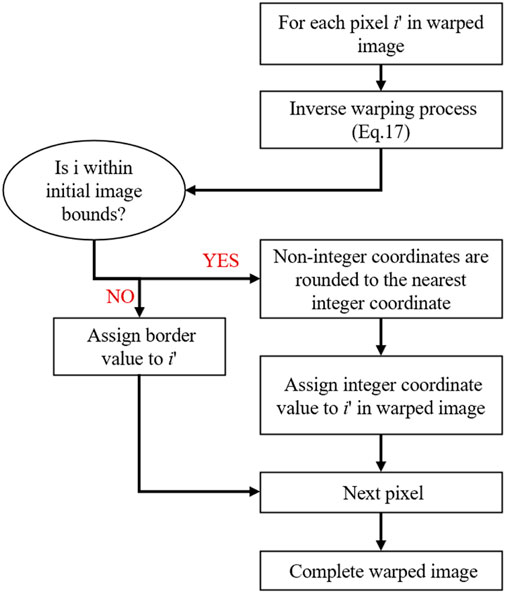
Figure 2. Flowchart of inverse warping.

2.3 Uncertainty quantification

The MRF model, as described by Wei and Wang (2022), incorporates local and global stratigraphical uncertainty. Epistemic uncertainty is introduced in the context of global uncertainty within an integrated image warping methodology. According to Steno’s law of superposition (Dominici et al., 2021), undeformed sedimentary stratigraphy is typically horizontal, with older layers underlying newer ones due to consistent depositional conditions. However, external forces and varying sedimentary conditions can deform these sequences, creating non-stationary stratigraphic fields. In engineering applications, regional geological knowledge from surveys, expert insights, and historical records, combined with on-site borehole data, enables the transformation of deformed stratigraphic sequences into undeformed profiles using image warping with selected control points. The MRF model then infers the undeformed stratigraphic profile, which is subsequently warped back to reconstruct the deformed profile.

Epistemic uncertainty, arising from subjective control point placement based on regional geological knowledge and borehole data, is addressed by assigning operational positions from a Gaussian distribution centered on preliminary positions.

To ensure statistical convergence of the global uncertainty, batch simulations are employed, with control point positions varying across simulations according to the predefined probabilistic distribution. Additionally, due to the uncertain burn-in period for granularity coefficients, a preliminary single simulation is recommended to determine the iteration count for the burn-in period before batch simulations (Wei and Wang, 2022).

After batch simulation, the robust majority vote (RMV) soil profile is determined using the majority vote principle (see Equation 18):

$\text{RMV}\left(i\right)={\mathrm{argmax}}_m\left(M{P}_i^{\left(m\right)};m\in \mathbf{L}\right)(18)$

where the $M{P}_i^{\left(m\right)}$ is the mean value of $P_i^{\left(m\right)}$ across the batch simulation, in which $P_i^{\left(m\right)}$ is the probability of unknown pixel $i$ chooses label $m$ within a single simulation and has the following Equation 19:

$P_i^{\left(m\right)}=\frac{N_i^{\left(m\right)}}{N_{ite}}(19)$

in which $N_{ite}$ is the total number of realizations in a single simulation, and $N_i^{\left(m\right)}$ is the number of realizations in which label $m$ is assigned at pixel $i$.

Global uncertainty at pixel $i$ is quantified using robust information entropy (RIE) defined by Equation 20 (Li et al., 2016):

$RI{E}_i=-{\displaystyle \sum _{m\in L}}\left[M{P}_i^{\left(m\right)}\log M{P}_i^{\left(m\right)}\right](20)$

Higher $RI{E}_i$ indicates greater uncertainty, making it harder to assign a soil label based on nearby borehole data. The RIE accounts for model uncertainty, cognitive uncertainty, and granularity coefficient uncertainty.

Simulation accuracy, when ground truth is available, is evaluated as Equation 21:

$Acc=\frac{{\sum }_{i=1}^{s}IN\left({x_i}^{\left(R\right)}={x_i}^{\left(T\right)}\right)}{s}(21)$

where $IN\left(·\right)$ = 1 if the simulated label at pixel $i$ (i.e., ${x_i}^{\left(R\right)}$) matches the ground truth label (i.e., ${x_i}^{\left(T\right)}$), and $s$ is the total number of pixels in the modeling domain.

3 Synthetic case studies

This section demonstrates the proposed methodology through a synthetic case, based on a 100 × 100-pixel “template profile” generated via Gibbs sampling with $\mathit{\beta }$ = [4.50, 0.15, 0.15, 0.15]. In this case, the profile is placed in an expanded spatial domain (Figure 3a) to simulate deformation. Five parallel series of control points (red points in Figure 3a) are set horizontally across the profile, with corresponding target points along five sinusoidal paths (Figure 3b). Image warping using these points produces a deformed soil profile (Figure 3c). The area within the white dotted box in Figure 3c serves as the “ground truth” profile. Four equidistant virtual boreholes (dashed lines in Figure 3d) are used to infer “unknown” pixel configurations.

Figure 3

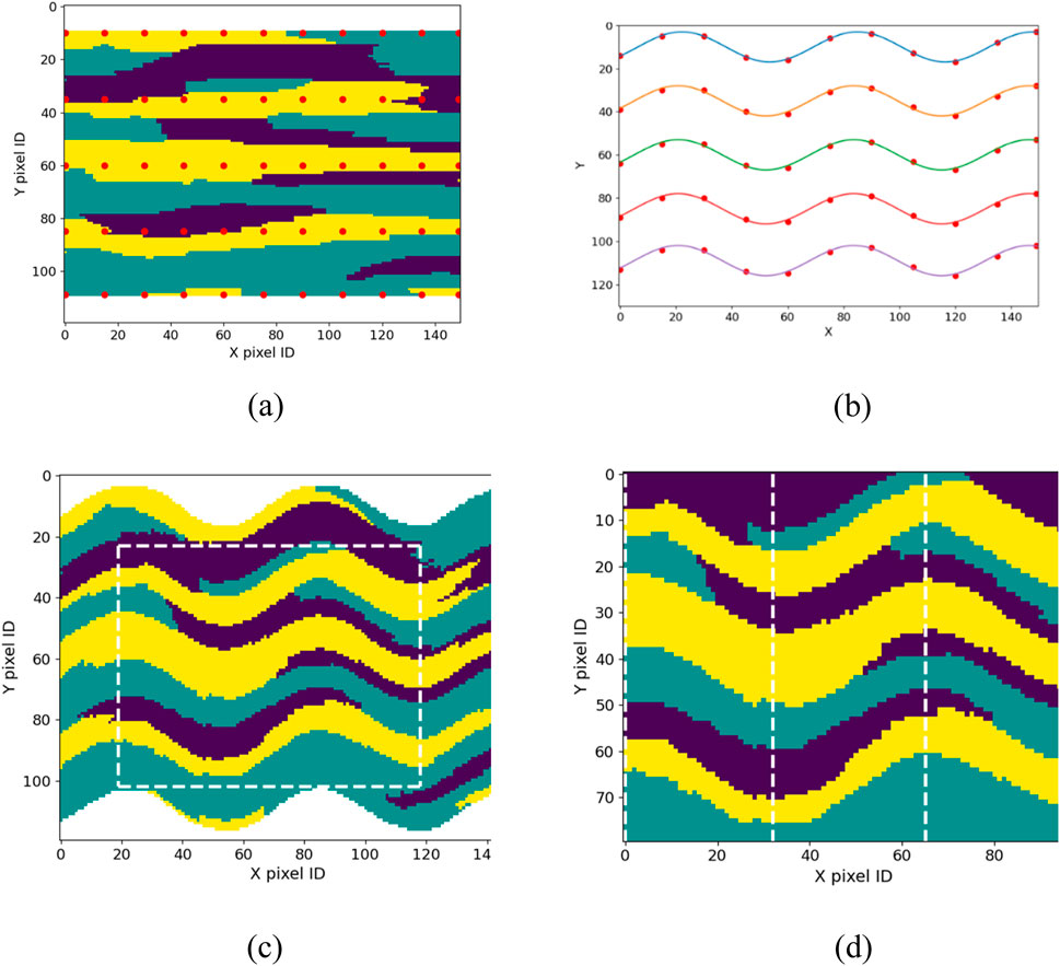
Figure 3. The deformation process of soil profile of the sinusoidal case. (a) Template profile (b) Five sinusoids (c) Warped soil profile (d) Original profile.

3.1 Warping of borehole information

Using regional geological data from surveys, expert insights, and historical records, the stratigraphic pattern is identified as having an approximately sinusoidal deformation. Three series of control points are placed on borehole pixels, aligned with this sinusoidal pattern (red dots on boreholes in Figure 3a). Additional control points (red dots off boreholes in Figure 3a) adjust the sinusoidal tangents to a horizontal orientation at the domain’s boundaries, based on geological inferences. Figure 3b shows the target points in standard space, illustrating the warped borehole information derived from these control and target points via image warping.

To account for epistemic uncertainty, operational positions of control points, drawn from a multivariate Gaussian distribution, are used for warping borehole information instead of preliminary positions. This distribution is defined by a mean vector ${\mathit{\mu }}_{CP}=\left.\left\{{\mu }_{CP}^i\right.\right|\left.i\in \left\{1,2,3,\dots ,\right.\left.N_{CP}\right\}\right\}$, where $N_{CP}$ is the number of control points, and a diagonal covariance matrix ${\mathbf{\Sigma }}_{CP}=diag\left({\left({\sigma }_{CP}^1\right)}^2,{\left({\sigma }_{CP}^2\right)}^2,{\left({\sigma }_{CP}^3\right)}^2,...,{\left({\sigma }_{CP}^{N_{CP}}\right)}^2\right)$, with each ${\sigma }_{CP}^i$ representing the standard deviation for the row indices of control points. Figure 3c shows a sampled instance from this distribution, displaying operational positions (red dots) alongside preliminary positions (blue dots). Figure 3d illustrates the target points and warped borehole information in standard space, based on the operational positions in Figure 3c.

3.2 Pre-test

As outlined in Subsection 2.4, a pre-test is required before conducting batch simulations. The prior distribution for granularity coefficients $\mathit{\beta }$ is set as $\mathit{\mu }$ = [1,1,1,1], $\mathit{\sigma }$ = [10, 10, 10,10], as posteriors are insensitive to priors and the interval $\left[\mathit{\mu }-3\mathit{\sigma },\mathit{\mu }+3\mathit{\sigma }\right]$ covers reasonable values of $\mathit{\beta }$ (Wei and Wang, 2022). The inferred posterior distribution of $\mathit{\mu }$ and $\mathit{\sigma }$, post-burn-in, are $\mathit{\mu }$ = [4.87, 0.21, 0.17, 0.08], $\mathit{\sigma }$ = [0.34, 0.36, 0.33, 0.28]. This posterior distribution serves as the prior for batch simulations, eliminating the burn-in period by enabling rapid convergence of the Metropolis-Hastings sampler (Wei and Wang, 2022).

To investigate the impact of initial β values on the converged posterior values, we conduct an additional test using an initial value set of $\mathit{\mu }$ = [6,6,6,6], $\mathit{\sigma }$ = [10, 10, 10,10]. The resulting posterior values are $\mathit{\mu }$ = [4.72, 0.18, 0.19, 0.11], $\mathit{\sigma }$ = [0.34, 0.26, 0.36, 0.31], which are nearly identical to those obtained previously and remain closely aligned with the “true values” [4.50, 0.15, 0.15, 0.15]. The two tests demonstrate that when the prior σ is set to a relatively large value, the posterior β values consistently converge to the vicinity of the “true values” during the MCMC sampling process, irrespective of the initial mean value.

3.3 Simulation outcomes analysis

The batch simulation, consisting of 100 Markov chains, yielded results shown in Figure 4. Convergence of global uncertainty is confirmed by the stabilization of total $RIE$ after approximately 40 simulations (Figure 4f). The RMV profile (Figure 4c) closely matches the original profile (Figure 3d), with discrepancies mainly at stratigraphic formation interfaces. Despite only 4 boreholes providing 4% of the total data, the RMV profile achieves 89.76% accuracy, remarkable given the complex synthetic soil configuration. The uncertainty map (Figure 4e) shows low uncertainty in core formation areas and higher uncertainty along interfaces, aligning with expected geological uncertainty patterns.

Figure 4

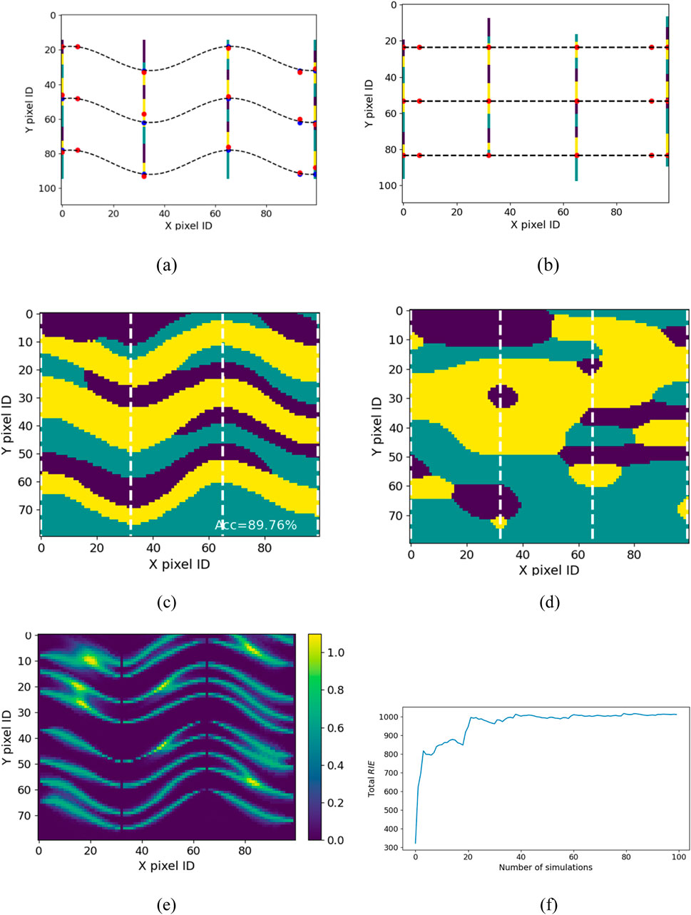
Figure 4. Boreholes and simulation results. (a) Boreholes in physical space; (b) Warped boreholes in standard space; (c) RMV via image warping; (d) RMV via no image warping. (e) RIE via image warping; (f) Total RIE versus number of simulations.

In contrast, the RMV profile without image warping (Figure 4d) significantly deviates from the original, underscoring the effectiveness of the proposed methodology in accurately modeling complex, non-homogeneous stratigraphic patterns.

To evaluate the impact of the epistemic uncertainty, we conducted experiments with different standard deviations (σ_CP) for the control points, specifically values of 1, 2, and 3. The resulting stratigraphic profiles exhibited comparable accuracy (i.e., 89.76%, 90.11%, 89.96%) across these settings, suggesting that the model’s performance is not highly sensitive to variations in the probabilistic distribution of control points. These findings support the model’s applicability under different parameter configurations.

4 Real-world case study

In this section, we investigate a geotechnical dataset extracted from the state of Kentucky, United States, referred to as the Kentucky case. This dataset serves as a practical illustration for assessing the effectiveness of the proposed approach within the realm of engineering applications. Figure 5a shows the collected borehole data (13 boreholes, four distinct soil types, no complete soil profile) of the Kentucky case.

Figure 5

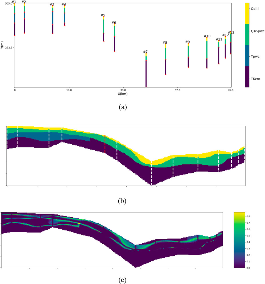
Figure 5. Case information and simulation results when #5 is the validation borehole. (a) Collected boreholes; (b) RMV (c) RIE.

To evaluate the model’s efficiency, a cross-validation approach is used, designating one borehole as the validation borehole and the remaining twelve as testing boreholes for stratigraphic estimation. Figures 5b,c show the RMV profile and corresponding RIE using borehole #5 for validation and boreholes #1–#4 and #6–#13 for testing, illustrating inferred slope stratigraphy within the region enclosed by lines connecting the slope surface to borehole bottom ends. The stratigraphy displays a tilted distribution aligned with the slope gradient, with low overall uncertainty but higher uncertainty at stratigraphic boundaries.

Cross-validation accuracies for all boreholes as validation boreholes are [0.83, 0.73, 0.78, 0.62, 0.74, 0.83, 0.82, 0.82, 0.94, 0.72, 0.90, 1.00, 0.96]. Most boreholes show satisfactory accuracy, with only borehole #4 below 70%. These results highlight the proposed approach’s strong performance in the Kentucky case, demonstrating its effectiveness in handling non-stationary fields in practical applications.

To further illustrate the performance of the proposed approach and compare the proposed approach with existing approaches, the published case from Shi and Wang (2021) extracted from a tunnel project in Australia (referred to as Australia case) are studied.

Figure 6a presents the complete soil profile and known boreholes (dashed lines) for the Australia case from Shi and Wang (2021). Eleven control points are placed at the formation boundaries along the boreholes, as shown in Figure 6b. Based on these points, two cubic curves and one quadratic curve are fitted to define the boundaries. Additionally, six control points are set on the curves at the left and right side of the modeling domain to adjust boundary tangents, ensuring horizontal tangents consistent with geological knowledge. These additional points are marked as red dots off the boreholes in Figure 6b Accordingly, one situation of the warped boreholes is shown in Figure 6c.

Figure 6

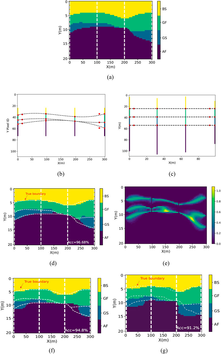
Figure 6. Australia case study. (a) Original field. (b) Known Boreholes. (c) Warped boreholes (d) RMV via image warping. (e) Corresponding RIE. (f) RMV via conventional MRF. (g) Reported profile (IC-XGBoost).

After simulation, the accuracy of RMV profile is 96.68% (see Figure 6d), which is, a remarkable result for this case with very sparse borehole information. The RIE image is shown in Figure 6e. It shows the high uncertainty level areas are concentrated at the boundaries and the pixels located in interior of each formation have extremely low uncertainty level. The results inferred with the conventional MRF-based model (Wei and Wang, 2022) and IC-XGBoost model (Shi and Wang, 2021) are shown in Figures 6f,g Showing the accuracy 94.8% and 91.2%. Obviously, the proposed approach, integrating image warping techniques, demonstrates superior performance with higher accuracy and produces strata lines that more closely align with the true boundary.

5 Concluding remarks

This study presents a novel approach integrating image warping with an advanced stratigraphic stochastic simulation model to characterize non-stationary fields and quantify associated stratigraphic uncertainties. The image warping technique, using thin plate splines and regional geological knowledge, transforms non-stationary fields into stationary ones, enabling the application of an in-house stratigraphic stochastic simulation model. The integrated approach effectively handles complex non-stationary stratigraphic conditions with limited data.

The synthetic and real-world cases validate the methodology’s effectiveness. Results show high accuracy in inferring complex non-stationary stratigraphy, with low and rationally distributed stratigraphic uncertainty, considering both local and global uncertainties, including model and cognitive uncertainties. The approach demonstrates strong applicability and potential for practical engineering applications.

Data availability statement

The original contributions presented in the study are included in the article/supplementary material, further inquiries can be directed to the corresponding author.

Author contributions

XW: Formal Analysis, Investigation, Methodology, Software, Writing – original draft, Writing – review and editing. HW: Conceptualization, Funding acquisition, Investigation, Methodology, Project administration, Software, Supervision, Writing – original draft, Writing – review and editing.

Funding

The author(s) declare that financial support was received for the research and/or publication of this article. This work is partially supported by Hunan Provincial Department of Education under the Project Number 24B0682 and Hunan Institute of Engineering under the Project Number 09001003/25069. This study was supported by the startup fund of the School of Engineering at the University of Dayton and the equipment fund from the Greg and Annie Stevens Intelligent Infrastructure Engineering Lab at the University of Dayton.

Acknowledgments

We also would like to acknowledge the support from Dr. Yichuan Zhu at Temple University for his inspiring discussion and kind case history data support to this work for testing the proposed approach.

Conflict of interest

The authors declare that the research was conducted in the absence of any commercial or financial relationships that could be construed as a potential conflict of interest.

Generative AI statement

The author(s) declare that no Generative AI was used in the creation of this manuscript.

Publisher’s note

All claims expressed in this article are solely those of the authors and do not necessarily represent those of their affiliated organizations, or those of the publisher, the editors and the reviewers. Any product that may be evaluated in this article, or claim that may be made by its manufacturer, is not guaranteed or endorsed by the publisher.

References

Bookstein, F. L. (1989). Principal warps: thin-Plate splines and the decomposition of deformations. IEEE Trans. pattern analysis Mach. Intell. 11, 567–585. doi:10.1109/34.24792

CrossRef Full Text | Google Scholar

Dominici, S. (2021). A Man with a Master Plan: Steno’s Observations on Earth’s History. Substantia 5 (1), 59–75. doi:10.36253/Substantia-1278

CrossRef Full Text | Google Scholar

Donato, G., and Belongie, S. (2003). Approximation methods for thin plate spline mappings and principal warps. Redwood City, CA: Digital Persona, Inc.

Google Scholar

Geman, S., and Geman, D. (1984). Stochastic relaxation, gibbs distributions, and the Bayesian restoration of images. IEEE Trans. pattern analysis Mach. Intell., 721–741. doi:10.1109/tpami.1984.4767596

PubMed Abstract | CrossRef Full Text | Google Scholar

Gong, W., Zhao, C., Juang, C. H., Tang, H., Wang, H., and Hu, X. (2020). Stratigraphic uncertainty modelling with random field approach. Comput. Geotechnics 125, 103681. doi:10.1016/j.compgeo.2020.103681

CrossRef Full Text | Google Scholar

Hastie, T., and Tibshirani, R. (1996). Discriminant adaptive nearest neighbor classification: IEEE Trans. Pattern Anal. Mach. Intell. 18, 607–616. doi:10.1109/34.506411

CrossRef Full Text | Google Scholar

Hastings, W. K. (1970). Monte carlo sampling methods using markov chains and their applications. Biometrika 57, 97. doi:10.2307/2334940

CrossRef Full Text | Google Scholar

Ioannou, P. G. (1988). Geologic exploration and risk reduction in underground construction. Journal of construction engineering and management, 114(4), 532–547. doi:10.1061/(ASCE)0733-9364(1988)114:4(532)

CrossRef Full Text | Google Scholar

Koller, D., and Friedman, N. (2009). Probabilistic graphical models: principles and techniques. Cambridge, Massachusetts: MIT press.

Google Scholar

Li, J., Cai, Y., Li, X., and Zhang, L. (2019). Simulating realistic geological stratigraphy using direction-dependent coupled markov chain model. Comput. Geotechnics 115, 103147. doi:10.1016/j.compgeo.2019.103147

CrossRef Full Text | Google Scholar

Li, Z., Wang, X., Wang, H., and Liang, R. Y. (2016). Quantifying stratigraphic uncertainties by stochastic simulation techniques based on markov random field. Eng. Geol. 201, 106–122. doi:10.1016/j.enggeo.2015.12.017

CrossRef Full Text | Google Scholar

Pan, Z., Wang, Y., and Ku, W. (2017). A new k-harmonic nearest neighbor classifier based on the multi-local means. Expert Syst. Appl. 67, 115–125. doi:10.1016/j.eswa.2016.09.031

CrossRef Full Text | Google Scholar

Qi, X.-H., Li, D.-Q., Phoon, K.-K., Cao, Z.-J., and Tang, X.-S. (2016). Simulation of geologic uncertainty using coupled markov chain. Eng. Geol. 207, 129–140. doi:10.1016/j.enggeo.2016.04.017

CrossRef Full Text | Google Scholar

Robertson, P. K. (1990). Soil classification using the cone penetration test. Can. geotechnical J. 27, 151–158. doi:10.1139/t90-014

CrossRef Full Text | Google Scholar

Shi, C., and Wang, Y. (2021). Development of subsurface geological cross-section from limited site-specific boreholes and prior geological knowledge using iterative convolution XGBoost. J. Geotechnical Geoenvironmental Eng. 147, 04021082. doi:10.1061/(asce)gt.1943-5606.0002583

CrossRef Full Text | Google Scholar

Shi, C., and Wang, Y. (2023). Data-driven sequential development of geological cross-sections along tunnel trajectory. Acta Geotech. 18, 1739–1754. doi:10.1007/s11440-022-01707-1

CrossRef Full Text | Google Scholar

Wang, H., Wellmann, J. F., Li, Z., Wang, X., and Liang, R. Y. (2017). A segmentation approach for stochastic geological modeling using hidden markov random fields. Math. Geosci. 49, 145–177. doi:10.1007/s11004-016-9663-9

CrossRef Full Text | Google Scholar

Wang, X., Wang, H., and Liang, R. Y. (2018). A method for slope stability analysis considering subsurface stratigraphic uncertainty. Landslides 15, 925–936. doi:10.1007/s10346-017-0925-5

CrossRef Full Text | Google Scholar

Wang, Y., and Zhao, T. (2017). Statistical interpretation of soil property profiles from sparse data using Bayesian compressive sampling. Géotechnique 67, 523–536. doi:10.1680/jgeot.16.p.143

CrossRef Full Text | Google Scholar

Wei, X., and Wang, H. (2022). Stochastic stratigraphic modeling using Bayesian machine learning. Eng. Geol. 307, 106789. doi:10.1016/j.enggeo.2022.106789

CrossRef Full Text | Google Scholar

Zhang, J.-Z., Liu, Z.-Q., Zhang, D.-M., Huang, H.-W., Phoon, K.-K., and Xue, Y.-D. (2022). Improved coupled markov chain method for simulating geological uncertainty. Eng. Geol. 298, 106539. doi:10.1016/j.enggeo.2022.106539

CrossRef Full Text | Google Scholar