Revisiting damping identification: limitations and comparative evaluation under impulse, white noise, and seismic excitations

Eigensystem Realization Algorithm (ERA), Stochastic Subspace Identification (SSI), Continuous Wavelet Transform (CWT), and Enhanced Frequency Domain Decomposition (EFDD) are four widely used damping identification methods. Their performance remains unclear in previous reviews and comparative discussions. This uncertainty can be attributed to three critical factors: the varying behavior of different methods under different excitations, the lack of a clear benchmark for evaluating accuracy, and the unquantified influence of parameter tuning on results. This study revisits and evaluates these methods under controlled conditions and addresses the key challenges that hinder reliable damping identification. A major challenge identified is the sensitivity of the results to parameter settings, which significantly impacts the stability and accuracy of the identification. Based on the evaluation, recommended methods and corresponding parameter guidelines are provided for three common excitation scenarios: impulse, white noise, and earthquakes. This study offers practical guidance for the selection and application of damping identification methods in structural dynamics.

1 Introduction

Damping describes energy dissipation in structural dynamic systems. Understanding it helps improve the accuracy of structural response simulations, since it could significantly affect the response on both global and local levels, such as base shear, roof displacement, inter-story drift, and floor acceleration (Lee, 2020a; Lee, 2022; Lee et al., 2023a; Lee et al., 2024a; Yang et al., 2025). It also provides valuable guidance for structural design codes (Cruz and Miranda, 2017), and helps to detect early damage (Daneshjoo and Gharighoran, 2008; Cao et al., 2017) because it reflects the impaired structural capability in energy dissipation.

Its composition is, however, often complex including internal structural material effects, dynamic friction between components and aerodynamic forces (Silva, 2007) and, therefore, the damping ratio of a structure cannot be derived directly from structural dimensions and material properties. In other words, the damping ratio could only be reliably obtained from measured vibration data through the use of damping identification techniques.

The identification of damping poses a greater challenge in comparison to the identification of structural frequencies or mode shapes (Xu et al., 2015). First, the composition of the damping mechanisms is often complex and the damping ratios identified from the same structure may not remain constant across different vibrations (Bernal et al., 2015). Second, identification methods are commonly developed based on viscous damping assumption (Adhikari, 2013). These methods are not well-suited to address the energy loss due to nonviscous mechanisms (Guo et al., 2022), particularly the nonlinear damage behavior caused by strong excitations like earthquakes (Dai et al., 2020). Third, the impact of noise on damping identification is more pronounced than that of other modal parameters such as structural frequencies and mode shapes (Bernal et al., 2015). Numerous identification methods have been developed to address these challenges, typically categorized into three domains: time, frequency, and time-frequency.

Among the time domain methods, the most representative is the logarithmic decrement. Several novel time-domain methods have also been developed, including the Eigensystem Realization Algorithm (ERA) (Juang and Pappa, 1985), Stochastic Subspace Identification (SSI) (De Moor et al., 1991) and Time Domain Decomposition (TDD) (Kim et al., 2005). ERA has been applied to seismic responses of a four-story building, demonstrating that damping ratios increase with larger earthquake amplitudes (Ulusoy et al., 2011). It has also been employed to analyze free vibrations of short telecom structures, revealing a relationship between damping and excitation amplitude (Jimenez Capilla et al., 2022). SSI has been used to detect structural damage by identifying damping ratios from measured ambient vibration responses of bridges (Yan et al., 2004). Attempts to enhance SSI through machine learning (ML) have been made, but improvements in damping ratio identification remain limited (Liu et al., 2023). TDD, although effective, does not directly utilize state-space models and has shown relatively lower accuracy in multi-modal analyses when compared to SSI for complex structural systems (Zahid et al., 2020).

Among the frequency domain methods, the half-power bandwidth method is the most well-known technique. The Enhanced Frequency Domain Decomposition (EFDD) (Brincker et al., 2001) is another famous frequency domain method which was easy to use and fast to process the data (Magalhães et al., 2010). It was applied to some high-rise buildings in Japan and revealed amplitude dependency of damping (Tamura et al., 2002; Tamura, 2012; Tamura et al., 2013).

Among the time-frequency domain methods, the Continuous Wavelet Transform (CWT) (Staszewski, 1997) and Hilbert-Huang Transform (HHT) (Huang et al., 1998) are two representative methods. CWT combined with Random Decrement Technique (RDT) was used to identify damping from seismic responses (Curadelli et al., 2008). CWT, when combined with the Random Decrement Technique (RDT), has been used to identify damping ratios from seismic responses, with results indicating that damping ratios are more sensitive than natural frequencies to changes in the structural damage state. This makes damping ratios more reliable indicators for damage detection (Curadelli et al., 2008). The accuracy of CWT combined with ERA in identifying a non-viscous damping was recently validated in an experimental vibration test of a cantilever beam (Shen et al., 2023). HHT, while effective in certain applications, suffers from limitations such as sensitivity to noise, instability in modal decomposition, and high computational complexity (Bao et al., 2009). For systems with closely spaced modes, CWT is theoretically more effective and reliable than HHT (Yan and Miyamoto, 2006).

Some studies have reviewed various damping identification methods (Zahid et al., 2020; Al-hababi et al., 2020; Papagiannopoulos and Beskos, 2012; Bin Abu Hasan et al., 2018), and some methods have been compared under certain cases recently (He et al., 2022; Peeters et al., 2000; Lew et al., 1993). However, these studies face three limitations: (1) The performance of identification methods based on different algorithms varies depending on the structural response under different excitations. These differences were not mentioned or distinguished. (2) These studies lack a clear benchmark for defining identification accuracy, leaving the comparison conclusion ambiguous. (3) Many methods require fine-tuning of specific parameters during the data processing. While some studies have acknowledged the influence of parameter settings on identification results (Zahid et al., 2020; Al-hababi et al., 2020), the extent of this impact has not been quantified.

To address the above-mentioned limitations, this study revisits and evaluates the performances of damping identification methods. It selects ERA, SSI, EFDD, and CWT due to their widespread application over the past few decades and compares their performance under three excitation scenarios: impulse, white noise, and seismic excitations. The data for analysis come from numerical simulations of a linear elastic multi-degree-of-freedom (MDOF) system. While real data, such as experimental results or recordings from instrumented buildings, are also available, the true damping ratios are unknown. In contrast, numerical simulations provide controlled conditions where the damping ratio is predefined, offering a clear benchmark for evaluating identification accuracy. Hence, the influence of parameter settings on identification accuracy can be quantitatively demonstrated. This study aims to provide a detailed evaluation of certain identification methods from the perspective of vibration signal analysis.

2 Criteria

The following shows the criteria used to evaluate the damping identification methods:

1. Noise robustness. In identifying modal parameters from structural responses, damping is more sensitive to noise than other modal parameters like natural frequencies (Ni et al., 2023; Bernal et al., 2012). Methods that exhibit strong noise robustness are crucial for ensuring reliable damping identification.

2. Higher modes: Damping for higher modes significantly influences inter-story drifts (Lee et al., 2023a), which are a crucial engineering demand to evaluate the damage of a building.

3. Sensor location: The ability to utilize response data from different sensor locations is essential because responses at various heights contain different modal damping information. Ideally, a method needs to leverage data from as many sensor locations as possible to ensure robust identification of multiple modal damping ratios.

4. Parameter sensitivity: All four methods require setting values for some parameters, but some of these recommended values have not been explicitly studied. Given that the accuracy of damping identification highly depends on the values of the parameters, it is important to find out the sensitivity of accuracy concerning the parameter values. The goal is not to give parameter recommendations but to compare the sensitivity of each method to the changes in these parameters. The way to qualify it is detailed later in Section 7.

3 Techniques of impulse response function extraction

ERA and CWT cannot be used to identify damping ratios from forced vibration responses as they only work for free vibration or impulse response. The following discusses two techniques for extracting impulse response function (IRF) from forced vibration response.

3.1 Natural excitation technique (NExT)

NExT was originally proposed for identifying the dynamic properties of structures based on ambient vibrations (James et al., 1993). It operates by computing the auto and cross-correlation functions between multiple time series recorded from different sensors.

Given two signals $x(t)$ and $y(t)$, their cross-spectral density is computed as $S_{xy}(\omega )=X(\omega )Y^{*}(\omega )$, where $X(\omega )$ and $Y(\omega )$ are the Fourier transforms of $x(t)$ and $y(t)$, and $Y^{*}(\omega )$ denotes the complex conjugate of $Y(\omega )$. The cross-correlation function $R_{xy}(\tau )$ can be obtained by applying the inverse Fourier transform to the cross-spectral density as $S_{xy}(\omega )$ and they both form a Fourier pair, as shown in Equation 1:

$S_{xy}\left(\omega \right)={\int }_{-\infty }^{\infty }{R}_{xy}\left(\tau \right)e^{-i*\omega }d\tau ,R_{xy}\left(\tau \right)=F^{-1}\left(S_{xy}\left(\omega \right)\right)(1)$

where time lag $\tau$ represents the delay between two signals $x(t)$ and $y(t)$. The cross-correlation function $R_{xy}(\tau )$ describes how similar or correlated the signals are when one is shifted in time relative to the other. It has the same characteristics as the system’s IRF (Hosseini Kordkheili et al., 2018; Zarafshan et al., 2014). In practice, $\tau$ is determined by engineers based on their experience. In this study, $\tau$ is treated as the parameter that affects the identification and its sensitivity will be investigated.

3.2 Random decrement technique (RDT)

RDT was originally developed by Cole (1971) at NASA in the late 1960s and early 1970s. The technique assumes that the random response of a structure at any given moment consists of three components: the step response resulting from initial displacements, the impulse response from initial velocity, and a random component caused by external forces.

RDT aggregates multiple segments of response data, known as Random Decrement (RD) segments, that share a common triggering condition $y_s$, a predefined threshold in displacement or velocity. The RD function (also named RD signature) can be expressed as Equation 2:

$\text{RD}\left(s\right)=\frac{1}{N}{\displaystyle \sum _{i=1}^N}{x}_i\left(t_i+s\right)(2)$

where $x_i(t_i+s)$ represents the response segments from time $t_i$ to $t_i+s$, $s$ denotes the time duration of each RD segment and $N$ is the number of segments which meet the triggering condition. The averaging process eliminates components related to initial velocity and forced vibrations (Asmussen, 1997), leaving only the contribution from the initial displacement. This RD signature can be treated as an IRF of the system for extracting the dynamic characteristics, including natural frequencies and damping ratios (Zhou and Li, 2021). The segment length $s$ and triggering condition $y_s$ are both user-defined parameters, which affect the accuracy of the identified damping ratio (Zheng et al., 2024a). Many researchers have provided their insights regarding the recommended parameters (Zhou and Li, 2021; Kijewski, 2000; Tamura, 2012; Tamura and Suganuma, 1996), but these are often limited to scenarios involving steady-state excitation. In this study, these two parameters will be investigated. The triggering condition is represented by the product of the standard deviation $(\sigma )$ of the response and a trigger coefficient, named trigger value.

4 Numerical data

This study relies on numerical simulations to generate response data. A 3-story flexure-type model with viscous damping is built in OpenSees (McKenna, 2011), as shown in Figure 1.

Figure 1

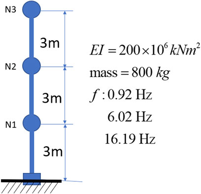
Figure 1. illustration of numerical model in OpenSees.

The flexure-type model can reveal well-separated modes, reducing the interference from closely spaced modes in each identification method. The model consists of a cantilever beam with three nodes, each with a lumped mass of 800 kg, accounting for horizontal mass inertia only. The beam spans 9 m in length, with Young’s modulus of $2\times 10^8$ kNm², and a cross-sectional dimension of 15 cm by 15 cm. The modal frequencies are 0.92 Hz, 6.02 Hz, and 16.19 Hz. The global damping ratio is assigned 2% for 3 modes by using the bell-shaped model (Lee, 2020a; Lee, 2019; Lee, 2020b; Lee, 2021; Lee et al., 2023b; Lee et al., 2024b). The responses under three excitation scenarios, namely, impulse, white noise and earthquake, are simulated by the Newmark constant acceleration method $(\beta =0.25,\gamma =0.5)$ with a time step of 0.005 s.

To test how sensitive the structural response, particularly the drift, is affected by damping ratios under strong earthquake excitation, the Tabas earthquake with its PGA of 1 g was introduced. Table 1 shows the relationship between the damping ratio and the relative error in the maximum drift at Node 3, the top node. When the damping ratio is within the 20% interval of the 2% damping, the corresponding drift is within the 5% interval of the drift with 2% damping. Therefore, 20% is set as the tolerance baseline in the following sections.

Table 1

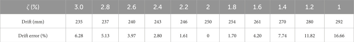
Table 1. Relative error of drift at Node 3 versus the damping ratios.

To maintain a coherent scope and a clear benchmark across methods, the present study intentionally confines the analysis to linear elastic systems. Under this controlled setting, several approaches would exhibit limited accuracy or pronounced parameter sensitivity under realistic seismic inputs, which will be discussed later. Extending them to nonlinear or damaged states is therefore nontrivial, and damping modelling or identification for softening structures remains challenging (Lee and Chang, 2022). Cases on structure with nonlinear and damage status will be addressed in a dedicated follow-up study.

5 Identification methods

5.1 Enhanced frequency domain decomposition (EFDD)

EFDD is an extension of the Frequency Domain Decomposition (FDD) method (Zahid et al., 2020). The process begins with estimating the power spectral density (PSD) of the measured responses, ${\text{PSD}}_{xx}(\omega )$, which provides an energy distribution of responses across different frequencies. It is then decomposed by singular value decomposition (SVD), as shown in Equation 3:

${\text{PSD}}_{xx}\left({\omega }_i\right)=U_i{S}_i{U}_i^{\text{H}}(3)$

where the matrix $U_i=\left[u_{i1},u_{i2},\dots ,u_{im}\right]$ is a unitary matrix holding the singular vectors, $S_i$ is a diagonal matrix holding the scalar singular values, $m$ is the number of measurements, and superscript $H$ is the complex conjugate and transpose. At the peak in the spectrum, the first singular vector $u_{i1}$ is an estimate of the mode shape for the corresponding mode. It can be regarded as the mode shape of the SDOF system decomposed from the original MDOF system. The PSD function of each SDOF system could be obtained using the bell-shaped peak selection method, employing the Modal Assurance Criterion (MAC), as shown in Equation 4, to ensure that the selected singular vector is well-matched to each SDOF system.

$\text{MAC}=\frac{{\left|{\varphi }_1^T{\varphi }_2\right|}^2}{\left({\varphi }_1^T{\varphi }_1\right)\left({\varphi }_2^T{\varphi }_2\right)}(4)$

where ${\varphi }_1$ and ${\varphi }_2$ are the two mode shape vectors being compared. The auto-correlation function can be obtained by applying the inverse Fourier transform to each determined SDOF-PSD function. The damping ratios are identified by applying logarithmic decrement to the auto-correlation functions of each SDOF system, as shown in Equation 5:

$\delta =\frac{1}{n}\ln \left(\frac{a\left(t\right)}{a\left(t+nT\right)}\right),\zeta =\frac{\delta }{\sqrt{4{\pi }^2+{\delta }^2}}(5)$

where $a(t)$ and $a(t+nT)$ are successive peak amplitudes of auto-correlation functions, and $n$ is the number of peak points utilized for constructing a fitting line. EFDD is sensitive to parameter selection at various stages, which can introduce bias in damping estimates (Bin Abu Hasan et al., 2018; Zheng et al., 2024b). In this study, MAC and the number of peaks $n$ are the parameters that are to be investigated.

5.2 Stochastic subspace identification (SSI)

SSI was developed with the capability to directly identify state-space models for systems subjected to stochastic excitation (Van Overschee and De Moor, 1996). It has high parameter estimation accuracy and computational efficiency compared to other methods (Reynders et al., 2016). The general procedure of SSI can be summarized in the following steps:

The first step involves constructing a Hankel matrix using the measured output data. The Hankel matrix $H_k$ is formed as Equation 6:

$H_k=\left(\begin{array}{cccc}\hfill y\left(k\right)\hfill & \hfill y\left(k+1\right)\hfill & \hfill \dots \hfill & \hfill y\left(k+n-1\right)\hfill \\ \hfill y\left(k+1\right)\hfill & \hfill y\left(k+2\right)\hfill & \hfill \dots \hfill & \hfill y\left(k+n\right)\hfill \\ \hfill ⋮\hfill & \hfill ⋮\hfill & \hfill \ddots \hfill & \hfill ⋮\hfill \\ \hfill y\left(k+m-1\right)\hfill & \hfill y\left(k+m\right)\hfill & \hfill \dots \hfill & \hfill y\left(k+m+n-2\right)\hfill \end{array}\right)(6)$

where $y(k)$ represents the system’s output data at time step $k$, and $n$ represents the time shift, which is also named block rows $(r_b)$. Then, the SVD was applied to the Hankel matrix $H$ to decompose it into three matrices $H=U\mathrm{\Sigma }{V}^T$, where $U$ and $V$ are orthogonal matrices, and $\mathrm{\Sigma }$ is a diagonal matrix containing the singular values. The matrix $\mathrm{\Sigma }$ ranks the energy or importance of each component in the data, with larger singular values corresponding to dominant dynamic modes.

At this point, the decomposition can be truncated by retaining only the most significant singular values and their corresponding vectors. This step allows us to reduce the noise in the data and focus on the dominant system behavior. The resulting truncated matrix, say ${\mathrm{\Sigma }}_r$, represents the reduced system’s dynamics. The matrix $U_r$ can be split into two parts, $U_p$ represents the data from past time steps and $U_f$ represents the data from future time steps. After that, a state-space model can be constructed as Equation 7:

$x\left(k+1\right)=Ax\left(k\right)+Bu\left(k\right),y\left(k\right)=Cx\left(k\right)+Du\left(k\right)(7)$

where $A$, $B$, $C$, and $D$ are the system matrices, $x(k)$ is the state vector, and $u(k)$ represents input data. The matrices $A$ can be computed as $A=U_f^{+}{U}_p$, where $U_f^{+}$ represents the Moore-Penrose pseudoinverse of $U_f$. The eigenvalue problem of matrix $A$ is solved to extract the system’s modal parameters, including natural frequency and damping ratio for each mode, as shown in Equation 8:

$A{\phi }_i={\lambda }_i{\phi }_i,{\zeta }_i=-\frac{\text{Re}\left({\lambda }_i\right)}{|{\lambda }_i|}(8)$

where ${\lambda }_i$ are the eigenvalues, ${\phi }_i$ are the eigenvectors and Re is the operator that extracts the real part of $\lambda$.

This method was improved later (Peeters and De roeck, 1999) into two algorithms: data-driven SSI (SSI-DATA) and covariance-driven SSI (SSI-COV). SSI-DATA usually provides better performance compared to SSI-COV (Li et al., 2018), as it uses the analytical spectrum expression and can predict future measured data through the implementation of a Kalman gain (Yan et al., 2004). However, the application of SSI-DATA requires careful parameter selection (Li et al., 2018). The block row $(r_b)$ is the parameter investigated in this study.

5.3 Eigensystem realization algorithm (ERA)

ERA is built upon Markov parameters, which are derived from the system’s impulse response function. These parameters are used to construct a block Hankel matrix, which allows for the realization of a discrete-time state-space model (Li et al., 2011). The ERA procedure begins with constructing a block Hankel matrix $H_k$, the same as Equation 6. The difference is that ERA used impulse response data to build this $H_k$.

Then, the SVD is applied to the block Hankel matrix: $H_k=U\mathrm{\Sigma }{V}^T$. The system order is determined by examining the singular values in $\mathrm{\Sigma }$. Singular values close to zero indicate noise and can be truncated. A reduced-order realization is constructed using the truncated SVD:$H_k\approx U_r{\mathrm{\Sigma }}_r{V}_r^T$, where $U_r$, ${\mathrm{\Sigma }}_r$, and $V_r$ correspond to the retained singular values and vectors. Then a shifted Hankel matrix $H_{k+1}$ is used to compute the system matrices $A$, as shown in Equation 9:

$A={\mathrm{\Sigma }}_r^{-\frac{1}{2}}{U}_r^T{H}_{k+1}{V}_r{\mathrm{\Sigma }}_r^{-\frac{1}{2}}(9)$

The eigenvalue problem of matrix $A$ is solved to extract natural frequencies and damping ratios, the same as Equation 8.

One challenge of ERA is selecting the optimal dimensions for the block Hankel matrix. Mathematically, this parameter has the same meaning as $r_b$ in SSI. However, in ERA, its value is significantly larger than in SSI, and this is more intuitively reflected in the response signal as a time lag. Improper selection can hinder the effective separation of the signal from noise (Juang, 1994). In this study, time lag, which determines the dimension of the Hankel matrix, is the parameter investigated in this study.

5.4 Continuous wavelet transform (CWT)

CWT is a time-frequency domain method, with its core principle centred on applying a wavelet function. This function is an adjustable waveform that can be shifted along the time axis and scaled along the frequency axis to extract time and frequency information simultaneously from the measured response data (Staszewski, 1997). The procedure of CWT can be briefly summarized as follows (Slavič et al., 2003):

First, the scale parameters of the wavelet function are adjusted to cover a range of frequencies relevant to the structural modes of interest. Then, the natural frequency can be computed using the classical Fourier transform. After that, the ridge is extracted, representing the energy concentration in the wavelet time-scale plane. The ridge $R(t)$ can be defined as the set of points where the modulus of the wavelet coefficients is maximised: $R(t)={\max }_a|W_x(a,t)|$, where $W_x(a,t)$ represents the wavelet coefficients. Then, the skeleton, which consists of the values of the wavelet transform restricted to its ridge, is extracted: $S(t)=W_x(a(t),t)$, where $a(t)$ is the scale corresponding to the ridge at time $t$. The envelope of the wavelet transform is computed to analyze the energy distribution over time: $E(t)=|S(t)|$. Finally, the damping ratio $\zeta$ is extracted by fitting the $E(t)\propto e^{-\zeta {\omega }_{n}t}$.

Like ERA, CWT is limited to damping identification from impulse response or free vibration. It is known for its resilience to noise and its ability to identify damping at closely spaced natural frequencies (Ruzzene et al., 1997). However, its computational complexity increases with the size of the data, potentially making it computationally demanding for long signals (Lamarque et al., 2000). In this study, the method using the Morlet wavelet proposed by Slavič et al. (2003) is selected. Although this method has been extended to other wavelets (Gabor (Wang et al., 2021) and Cauchy (Erlicher and Argoul, 2007)), Morlet wavelet is widely used and discussed (Curadelli et al., 2008; Ta and Lardiès, 2006; Chen et al., 2009; Wang et al., 2024), making it a valuable benchmark for comparison in this study. The numerical simulation data provides a sufficiently long duration to ensure the performance of the CWT method. The method of CWT does not require parameters to be investigated in this study.

6 Comparison under impulse excitation

This section compares the four methods based on criteria 1, 2 and 3. Criterion 4, parameter sensitivity, is not considered in this part, as the damping identified from the impulse response is not sensitive to it. According to Equation 7, under the state space system assumption, $Bu(k)$ and $Du(k)$ represent the process and measurement noises (Yan et al., 2004). Therefore, two types of noise are considered: one adding to the excitation source and the other adding to the measurement data.

Response datasets containing displacement and acceleration recordings from three nodes are collected. Three cases are considered: (1) Case (II), Idealized Impulse response. The impulse is a 1 g acceleration ground excitation with a 0.1 s period. (2) Case (IM), Impulse response with Measurement noise. The measurement noise is set to Gaussian white noise with a signal-to-noise ratio (SNR) of 35 dB, which is an acceptable setting for the accelerometers (Brincker and Ventura, 2015). (3) Case (IEM), Impulse response with Excitation noise and Measurement noise. The Excitation noise is set to a slight Gaussian white noise with a standard deviation of 0.01 g. This is to simulate the slight ground disturbance in the experimental environment.

All datasets are processed using a Butterworth low-pass filter with a cutoff frequency of 60 Hz. The relative errors of identified damping using the methods CWT, ERA and SSI, for the three cases II, IM, and IME, are given in Table 2.

Table 2

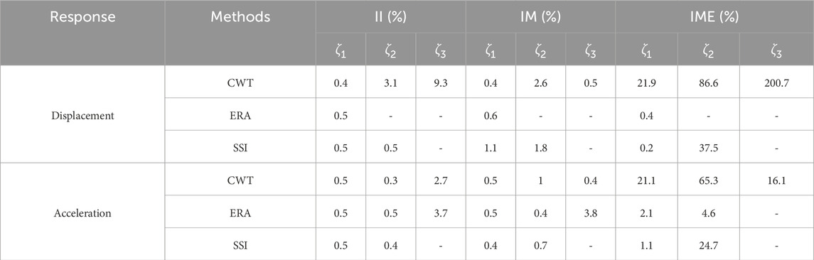
Table 2. Relative errors of three methods using two types of responses in Cases II, IM, and IEM.

Not all results are reported in Table 2 because (1) The EFDD method could not effectively identify damping ratios from impulse response signals. The impulse excitation lasts a short time, expressing weak information at the resonance peaks in the spectrum, causing inaccuracies in damping identification. (2) The accuracy of SSI-DATA is significantly superior to that of SSI-COV. Therefore, the SSI in Table 2 are presented with SSI-DATA results. (3) ERA and SSI can analyze multi-channel inputs, but CWT can only process single-channel inputs. The response of different nodes reveals different results by CWT (Mazza et al., 2023), as shown in Table 3. Node 1 (the node immediately above the fixed ground support) displacement records and node 3 (the top node) acceleration records reveal better results than other records. The optimal choice, namely, node 1 displacement records and node 3 acceleration records, are selected to be reported in Table 2 for CWT.

Table 3

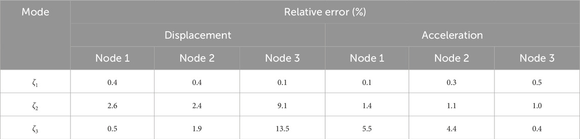
Table 3. Relative errors of CWT using responses of different types and nodes in Case IM.

The identification results are reported in Table 2 as relative errors. It shows that when displacement records are used, CWT performs well in the II and IM scenarios. SSI can identify two modal damping ratios and ERA can only identify the first one. None of them performs well in the IME scenario. When using acceleration records, ERA is the only method capable of identifying the first and second modal damping ratios in the IME scenario. It also provides accurate identification in both II and IM scenarios. SSI loses identifying damping ratios of the third mode but demonstrates accurate identification of damping ratios for the first two modes in II and IM. CWT fails to identify damping in the IME scenario but still performs better than SSI in II and IM scenarios.

According to the above discussions, Table 4 summarizes the performance ranking of these methods based on subjective quantitative analysis (SQA).

Table 4

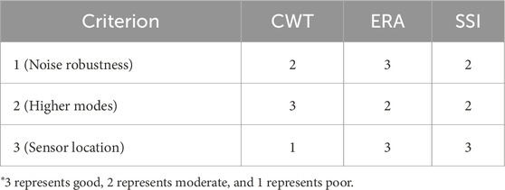
Table 4. Performance of methods in impulse excitation scenario.

Recommendations for damping identification of impulse response signals are as follows:

1. When the environmental noise level is low and acceleration records are available, ERA is recommended, with CWT as a supplementary verification. If only displacement records are available, CWT is recommended.

2. When the environmental noise level is high, ERA is recommended, with SSI as a supplementary verification.

7 Comparison under white noise excitation

The four methods are compared based on all four criteria. EFDD and SSI can be directly used to identify damping ratios from white noise responses. ERA and CWT must be combined with the impulse response function extraction techniques (IRFTs) mentioned in Section 3. Therefore, The following are considered: (1) EFDD, (2) SSI and methods combining SSI with IRFT, (3) Methods combining ERA with IRFT, and (4) Methods combining CWT with IRFT.

The affecting parameters are discussed in the introduction of each IRFT and method in Sections 3 and 5. NExT has one parameter, time length $\tau$. RDT has two parameters, trigger value $y_s$ and segment length $s$. EFDD has two parameters, MAC and the number of peaks $n$. SSI has one parameter, block row $(r_b)$. ERA has one parameter, time lag.

SSI, ERA, and CWT performed well under both II and IM conditions in the scenario of impulse response. Therefore, when discussing the methods combining SSI, ERA, and CWT with IRFT, only the parameters of IRFT will be considered. Fifty sets of Gaussian white noise, each lasting 200 s to ensure a stable performance of each method, are generated as excitation for simulation with acceleration responses recorded. In practice, using displacement sensors to collect responses under white noise excitation is rare, so this section will not compare the performance based on displacement records.

The analysis in this section will be divided into three steps. In step 1, each method is applied to several sets of responses. The reasonable parameter ranges for each method are determined through trial and error. The limit for each parameter is established at the point where a significant drop in identification accuracy occurs. This range will be shown later in the figures and will not be listed. In step 2, the procedure of trial and error is repeated across all the generated responses in the corresponding parameter range. The proportion of parameter settings that yield identification errors within the error tolerance of 20% across the whole trial is referred to as the satisfactory rate (SR). A higher SR indicates that the corresponding parameter setting is more likely to result in a damping ratio error below 20%. A more concentrated distribution of high SR values indicates that the method performs consistently well across a specific cluster of parameter settings. This consistency makes it easier for users to select appropriate parameters, ensuring stable identification accuracy. In step 3, the parameter settings that yield a high SR for the first and second modes are considered the recommended parameters. The methods assigned with the recommended parameter settings are applied to another set of white noise excitation responses to compare their noise robustness.

Figure 2 illustrates the EFDD results of the second step. The horizontal and vertical axes represent two parameter settings influencing the EFDD identification results. The color gradient indicates the value of the SR, which represents the probability that the EFDD identification results under the given parameter setting achieve an error below 20% across 50 runs.

Figure 2

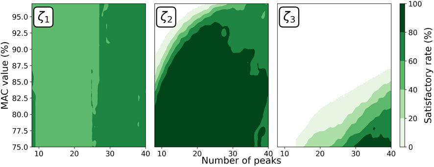
Figure 2. Satisfactory rate of EFDD versus the affecting parameters for all three modal damping ratios.

Figure 2 shows that the number of peaks mainly influences the damping ratio of the first mode. EFDD shows its stability in identifying the first and second modal damping ratios with SR exceeding 60% and 80%. The SR for the third modal damping ratio shows an increasing trend as MAC decreases. However, a very low MAC would introduce significant noise during the inverse Fourier transform process. The trend presented may be a coincidence specific to this model and damping ratio setting. Hence, EFDD cannot identify the damping ratio of the third mode of this model.

Figure 3 illustrates the SSI results in the second step. The trend lines in the figures are selected based on the best fit for the results, which could be either linear, polynomial, or piecewise. The trend lines show that the SR of SSI for the first modal damping ratio gets a peak when $r_b$ increases to around 30. The damping ratio identification for the second mode is very stable. When $r_b$ is between 29 and 34, the identified damping ratios for both the first and second modes exhibit a high SR. SSI fails to identify the third modal damping ratio.

Figure 3

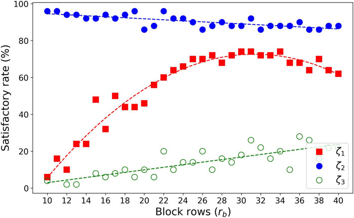
Figure 3. Satisfactory rate of SSI versus $r_b$ for all three modal damping ratios.

Figure 4 shows that for SSI + NExT, the SR exhibits small fluctuation in the identification of the first and second modal damping ratios. Compared to Figure 3, there is a noticeable decline in the SR for both the first and second modal damping ratios. While Figure 4 shows that the SR for the first mode damping ratio fluctuates more steadily with parameter variations and that the third mode damping ratio has improved, these advantages are minimal.

Figure 4

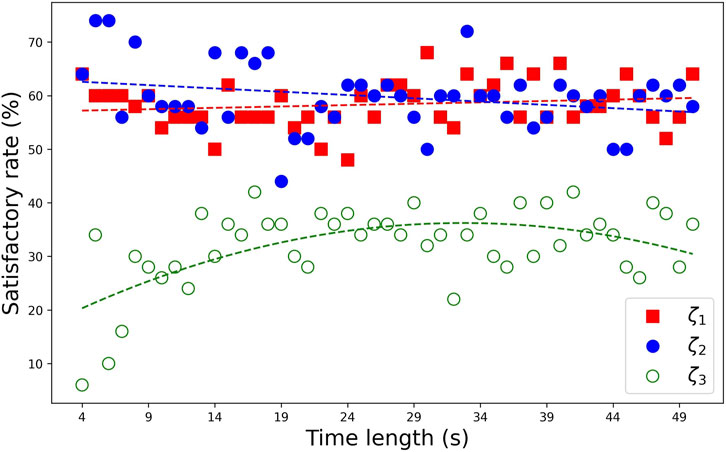
Figure 4. Satisfactory rate of SSI + NExT versus the time window length for all three modal damping ratios.

Using NExT to extract IRF as a supplement to SSI identification does not appear to give a better performance. Intuitively, adjusting $r_b$ value on SSI while using NExT might yield better results. However, doing so would undermine the purpose of evaluating the quality of the extracted IRF. Therefore, only the parameter affecting NExT is considered here.

Figure 5 shows that SSI + RDT performs well for the first and second modes but poorly for the third mode. The distribution of the SR across the parameter settings shows a certain pattern, but the concentration of high SR is not pronounced. Compared to SSI, the only advantage of SSI + RDT over SSI is a slight improvement in the SR for the third mode damping ratio. However, its performance in identifying both the first and second modal damping ratios is inferior. Therefore, using RDT to extract IRF as a supplement to SSI identification is also not a favourable option.

Figure 5

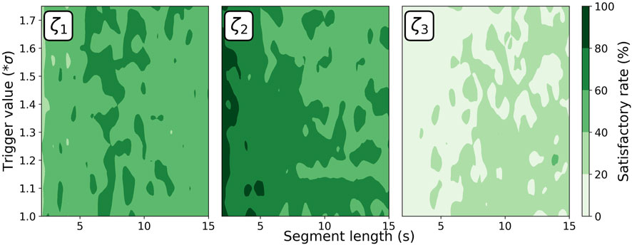
Figure 5. Satisfactory rate of SSI + RDT versus the affecting parameters for all three modal damping ratios.

Figure 6 demonstrates the capability of ERA + NExT to reliably identify the damping ratios of all three modes. The high SR distribution corresponding to the damping ratios of the three modes is easily found in concentrated areas. The superior performance of ERA + NExT lies in the overlap of these highly SR distributions, in the time segment from 1.2 to 1.7 s. This indicates that when the NExT parameter is set within this range, there is a high probability of simultaneously obtaining damping ratios for all three modes with errors below 20%.

Figure 6

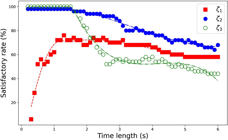
Figure 6. Satisfactory rate of ERA + NExT versus the time window length for all three modal damping ratios.

Figure 7 shows a trend where, as the modal order increases from 1 to 3, the region with high SR shifts towards smaller segment lengths. When identifying the damping ratios of higher modes, setting the RDT time segments short can ensure that high-modal information dominates the processed signal. This indicates that a unified parameter setting should not be used for identifying the damping ratios of multiple modes with ERA + RDT. Although ERA + RDT also demonstrates the capability to identify the three modes, its concentration of high SR distribution is slightly inferior compared to ERA + NExT.

Figure 7

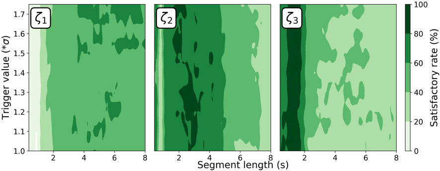
Figure 7. Satisfactory rate of ERA + RDT versus the affecting parameters for all three modal damping ratios.

When CWT is combined with NExT, the parameter under discussion initially is the time length, same as SSI + NExT and ERA + NExT. However, as mentioned in Section 3, CWT requires a long signal duration to ensure accurate identification. Through trials, it was observed that the accuracy of CWT + NExT increases with the time length and eventually converges. Therefore, the time length no longer holds significance for further discussion. On the other hand, CWT can only process single-channel responses. The responses composed of recordings from three nodes yield nine IRFs after NExT processing. The SR distribution results after analysing the nine IRFs are shown in Figure 8. This figure shows that the choice of IRF has little impact on the damping identification of the first mode. Although the CWT + NExT method performs poorly for the first modal damping, it demonstrates high SR in identifying the second and third modal damping ratios. This characteristic has not been mentioned in other studies, and its generality remains to be explored in the future.

Figure 8

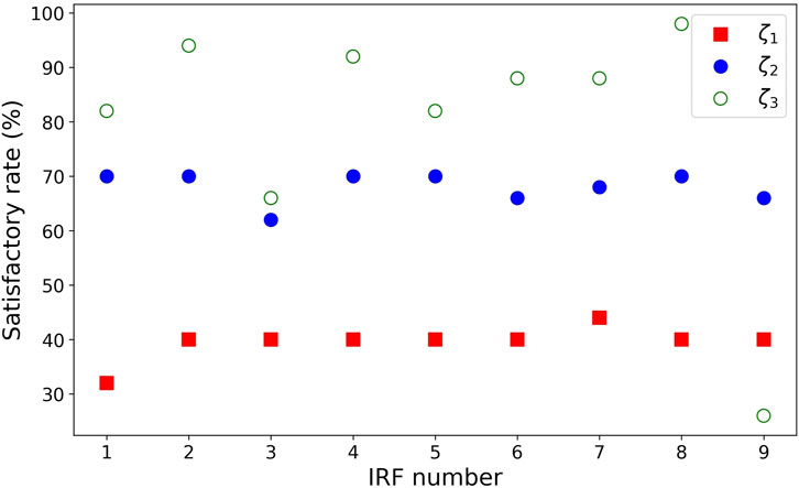
Figure 8. Satisfactory rate of CWT + NExT versus the IRF order for all three modal damping ratios.

The discussion for CWT + RDT should have originally focused on the parameters influencing RDT, namely, the segment length and triggering condition $y_s$. Similar to CWT + NExT, the accuracy of CWT + RDT increases with the segment length and eventually converges. Now only the triggering condition $y_s$ remains relevant for further discussion. Additionally, CWT can only process single-channel response data but RDT extracts three IRFs from the response recorded at the three nodes. Figure 9 shows the differences in identification accuracy of the CWT + RDT method for one sample set of responses at three nodes. The identification results for the response at node 3 exhibit advantages in both the first and second modes. Therefore, the response data at node 3 are used for the 50 identification tests. Figure 10 shows that the performance of CWT + RDT for the damping ratio identification of all three modes is unsatisfactory.

Figure 9

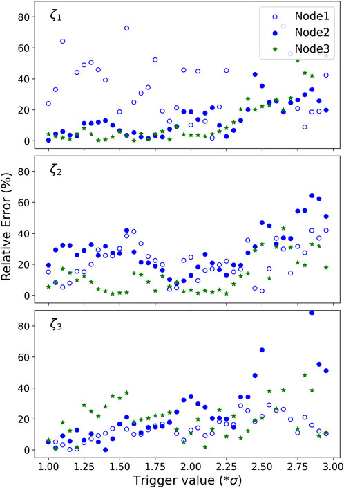
Figure 9. Error of CWT + RDT versus parameters for one set of responses at three nodes.

Figure 10

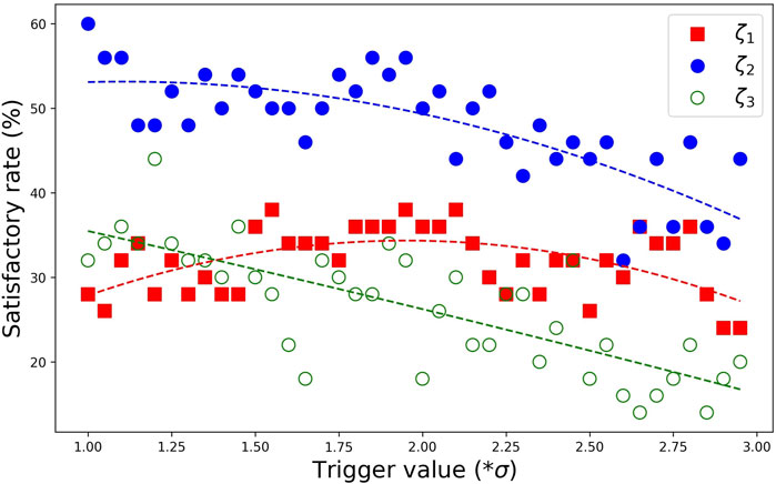
Figure 10. Satisfactory rate of CWT + RDT versus the trigger value for all three modal damping ratios.

In step 3, the parameter settings that yield the highest SR for the first and second modes are considered the recommended parameters, as shown in Table 5. Two sets of responses are generated. (1) The White noise excitation response (WN). The white noise excitation signal is set to Gaussian white noise with a standard deviation of 0.1 g. (2) White noise excitation response plus measurement noise (WNM). The measurement noise is set to Gaussian white noise with an SNR of 35 dB. All datasets are processed using a Butterworth low-pass filter with a cutoff frequency of 60 Hz. The results of these methods assigned with the parameters in Table 5 for the WN and WNM datasets are shown in Figure 11. The vertical axis accuracy is computed as $\text{Accuracy}=1-{\log }_{20}(\text{Relative\hspace{0.17em}error})$, where the relative error is in percentage. When the error exceeds 20%, the accuracy will be a negative value.

Table 5

Table 5. Parameter setting recommendations for each method under white noise tests.

Figure 11

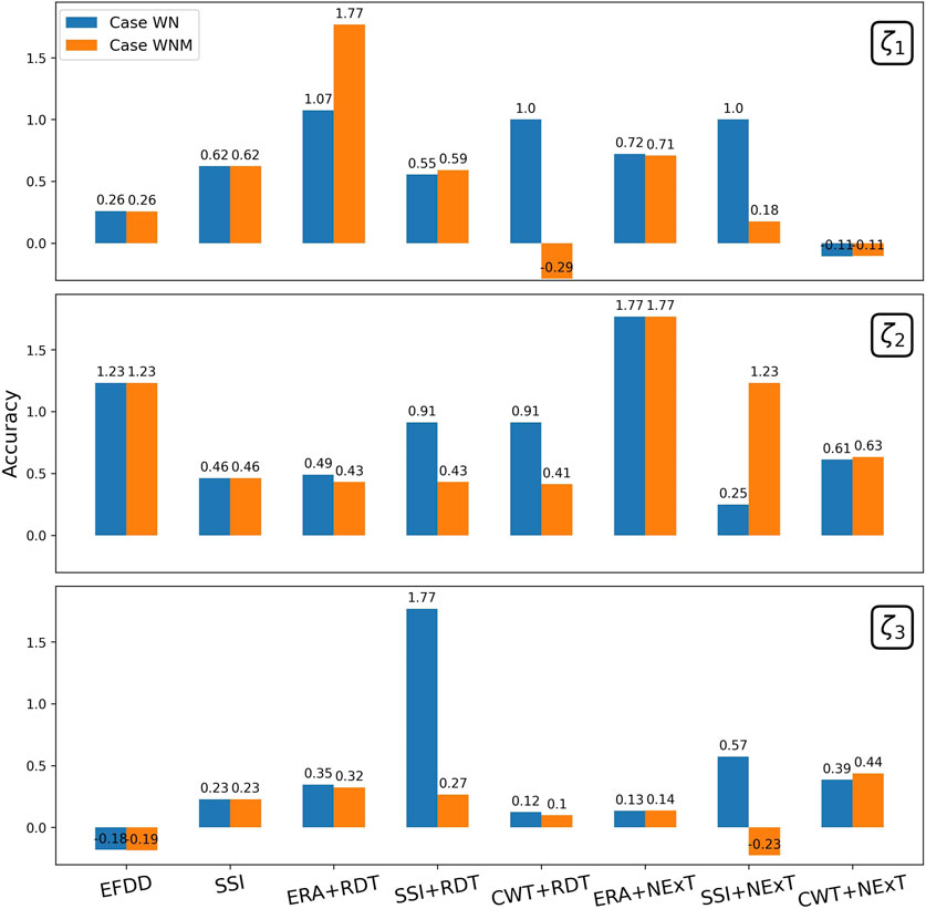
Figure 11. Accuracy of all methods in WN and WNM cases for all three modal damping ratios.

Figure 11 shows that EFDD, SSI, ERA + RDT, SSI + RDT, ERA + NExT and CWT + NEXT perform well on noise robustness. Their accuracy values in WN and WNM cases are consistent. Among them, SSI, ERA + RDT and ERA + NEXT have a relatively higher accuracy compared with the others. Table 6 summarizes the performance ranking of these methods based on SQA.

Table 6

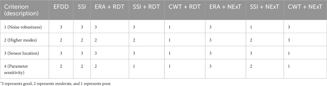
Table 6. Performance of methods in white noise excitation scenario.

In summary, ERA + NExT demonstrates a significant advantage in damping identification across all three modes. It is the first recommendation for damping identification from acceleration records under white noise excitation. EFDD and SSI perform well in identifying the damping ratios of the first and second modes, following ERA + NExT. They both can serve as verification methods. Comparing the results of SSI, SSI + RDT, and SSI + NExT shows that these two IRFTs do not provide noticeable improvements in SSI identification accuracy or parameter stability. The identification accuracy of CWT + RDT is not satisfactory, which may be related to the choice of the wavelet type. The consistently high accuracy of CWT + NExT in identifying the third mode is noteworthy.

8 Comparison under earthquake excitation

In this section, four methods are compared based on criteria 4 only. The analysis in this section fully follows the second step outlined in Section 7. Two hundred thirty-four earthquake recordings, obtained from the Center for Engineering Strong Motion Data (CESMD), were used as excitation sources. This data was used by Bernal et al. (2012) for discussing damping predictors of different types of structures.

To extend the scope of this study, models with varying natural frequencies were obtained by adjusting the mass at the nodes. The natural frequencies of these four models are as follows [0.92, 6.02, 16.19] Hz, [1.39, 9.11, 24.47] Hz, [1.84, 12.05, 32.37] Hz, and [2.6, 17.04, 45.78] Hz. When the error tolerance was set to the same 20% as in the previous section, all methods performed poorly, even for the identification of the first modal damping. Only EFDD, SSI, and SSI + RDT methods achieved satisfactory rates around 50%, while other methods fell below 40%. After relaxing the error tolerance from 20% to 50%, which means the error for the global drift would increase from 4.2% to 16.66% as shown in Table 1, these three methods continued to yield the highest satisfactory rates. Figures 12, 13 show the performance of EFDD and SSI across the four models after the error tolerance was relaxed to 50%. Since the results of SSI + RDT did not show any advantage over SSI and performed significantly worse in identifying the second modal damping ratio, consistent with the findings in Section 7, the results of SSI + RDT have been omitted here.

Figure 12

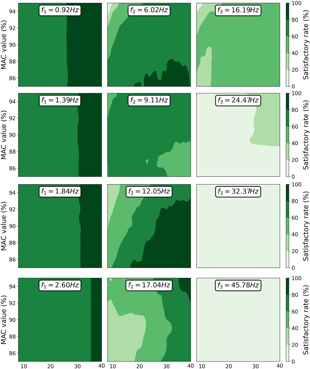
Figure 12. Satisfactory rate of EFDD versus the affecting parameters for all four models.

Figure 13

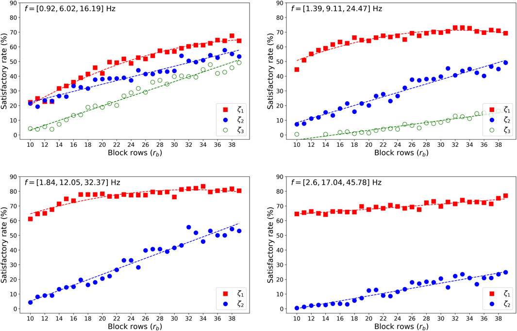
Figure 13. Satisfactory rate of SSI versus the $r_b$ affecting parameters for all four models.

Figure 12 shows that EFDD can reveal the damping ratio of the first and the second modes within an error of 50% in nearly 90% of the 234 tests. A higher number of peaks remains beneficial for the accuracy of the damping ratio for the first mode, consistent with the trends observed in the white noise section. As the structural modal frequencies increase, the accuracy of identifying the damping ratios for the third mode decreases sharply. There is no clear pattern in the variation of the optimal parameter setting region for the damping identification of the second mode. The third modal frequency of the first structure is close to the second modal frequency of the fourth structure, yet the damping identification results differ significantly. This suggests that the damping ratio identified by EFDD is more influenced by the mode order rather than the modal frequency.

Figure 13 shows that SSI has a lower satisfactory rate in identifying the damping ratio for the first mode compared to EFDD, with an even larger discrepancy for the second mode. As the structural modal frequency increases, SSI loses its ability to identify the damping of the highest mode. Since SSI requires adjusting only one parameter, while EFDD involves adjusting two parameters, the parameter sensitivity for identifying the damping ratio of the first mode is roughly comparable between the two methods. However, for the second mode, EFDD demonstrates a clear advantage compared to SSI.

In some previous studies, parameter setting recommendations derived from statistical analyses under noise or light wind excitation conditions have commonly been applied to damping identification for seismic responses (Yang et al., 2025; Curadelli et al., 2008; Frizzarin et al., 2010; Zhang and Cho, 2009). To explore this issue, one earthquake recording not included in the initial set of 234 was selected: the NZ2010 earthquake recorded at Darfield High School. This earthquake on 4 September 2010 (magnitude 7.0–7.1) and the destructive aftershock on 22 February 2011 (magnitude 6.3) caused significant loss of life and property for the residents of Christchurch. Parameter recommendations for the seismic scenario are derived based on the first structural settings corresponding to the highest satisfactory rate in the first mode results, as shown in Table 7. The identification results using the white noise recommendation values from the previous section will serve as the comparison group. Table 8 shows the identification results using parameter recommendations from Table 5 (white noise - WN) and Table 7 (earthquake - EQ).

Table 7

Table 7. Recommended parameter values of each method for earthquake excitations.

Table 8

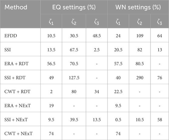
Table 8. Relative errors by all methods with recommended parameter values for earthquake NZ2010.

Under the condition of applying the EQ recommendation values, the performance of EFDD, SSI, CWT + RDT, ERA + NExT, and SSI + NExT are acceptable. They give the first modal damping ratio with less than 20% error. CWT + RDT provided the most accurate results for the damping ratio of the first mode. SSI and SSI + NExT provided good results for the damping ratio of the third mode. Under the condition of using the WN recommendation values, the performance of SSI, ERA + NExT, and SSI + NExT are acceptable. SSI + NExT provided the most accurate results for the damping ratio of the first and second modes. SSI provided good results for the damping ratio of the third mode. The identification accuracy of EFDD, SSI, and CWT + RDT improved when applying the EQ recommendation values. ERA + NExT and SSI + NExT provided more accurate results when applying the WN recommendation values.

In this case, CWT + RDT, ERA + NExT, and SSI + NExT outperformed EFDD and SSI, contrary to the statistical results from the 234 tests. It indicates the high degree of variability in the damping identification from seismic responses. Applying the EQ recommendation values has a positive effect on improving identification accuracy. The lack of a pronounced effect may be due to insufficient test samples.

In summary, EFDD remains the most stable method recommended for earthquake scenarios. SSI can be used as a verification method. When structural measurement channels are limited, such as having data from only one floor, CWT + RDT becomes a viable option.

As a side study, two additional numerical models were analysed to examine the generality of this comparative study: (i) a 2-storey flexure-type model from the authors’ previous work (Zheng et al., 2024b) and (ii) a 10-storey chimney model from Lee (2020a). The same bell-shaped proportional damping model was applied, with all modal damping ratios set to 2%. The results in Table 9 show that, although the absolute error magnitudes vary with structural type and modal order, the relative performance ranking among methods is generally consistent with that observed in the main models. EFDD and SSI remain among the most stable methods for the first modal damping ratio. Methods involving RDT exhibit large errors in several modes, confirming their sensitivity. ERA + NExT again yields good results, particularly for the first mode of the 10-storey chimney, but performance drops for other modes, reflecting the parameter sensitivity highlighted in Section 8. These findings suggest that the comparative conclusions drawn from the primary numerical model are not specific to that configuration but are also applicable to other structural types with different dynamic characteristics.

Table 9

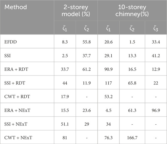
Table 9. Relative errors with recommended EQ settings for side study models under earthquake NZ2010.

9 Conclusion

Based on the criteria of noise robustness, higher modes, sensor location, and parameter sensitivity, this study compared the performance of EFDD, SSI, ERA, and CWT, in damping identification for the scenarios of impulse, white noise, and earthquake excitations. SSI, ERA, and CWT were combined with RDT and NExT when applied to a forced vibration analysis. Some conclusions revealed by the numerical test are as follows:

1. For the impulse excitation scenario, ERA demonstrated high accuracy and strong noise resistance when applied to acceleration records. CWT showed advantages when applied to displacement records, commonly collected in laboratories.

2. For the white noise excitation scenario, ERA + NExT performed best. Its remarkable performance in parameter sensitivity could allow users to select appropriate parameters to achieve satisfactory identification accuracy more easily. The next best are EFDD and SSI.

3. For the earthquake excitation scenario, both EFDD and SSI performed well in terms of stability without being too sensitive to the choice of parameter values. Their performance on accuracy is not fully satisfactory.

4. Applying a fixed set of parameter settings to identify the damping ratios of multiple modes is not ideal for all methods. Determining parameter recommendations tailored to different modes based on structural diversity requires extensive study.

5. In a certain case under NZ2010 earthquake excitation, some recently proposed methods, such as CWT + RDT, performed better than EFDD and SSI in accuracy, but might not exhibit stability. Hence, using one method alone for damping identification with seismic responses poses risks. It would be worthwhile to explore an approach to combine the stability of EFDD with the high accuracy of novel methods in the future.

6. Compared to the parameter recommendations obtained from the statistical analysis of white noise responses, applying the parameters derived from the statistical analysis of seismic responses significantly improves the identification accuracy of EFDD, SSI, and CWT + RDT methods. More extensive modelling and statistical analysis of earthquake responses are needed in the subsequent studies.

This study provided clear strategies by statistical analysis to address damping identification for the impulse, white noise, and earthquake excitation scenarios. The methods used in this study are mathematically based on the formulations shown in Section 5, whereas many subsequent improvements have been made by several researchers (Ulusoy et al., 2011; Li et al., 2018; Brincker and Amador, 2022; Qu et al., 2024; Bajrić and Høgsberg, 2018; Huang and Gu, 2016; Dou et al., 2016). Nonetheless, this study comprehensively evaluates the performance of each method based on the established criteria with a benchmark. It can serve as a useful guide for researchers who wish to apply these methods in their studies involving damping identifications. The parameter recommendations derived from the statistical analysis of 236 earthquake responses can also serve as references.

Data availability statement

The raw data supporting the conclusions of this article will be made available by the authors, without undue reservation.

Author contributions

YZ: Formal Analysis, Data curation, Visualization, Writing – original draft, Validation, Conceptualization, Investigation, Methodology. C-LL: Resources, Methodology, Project administration, Conceptualization, Writing – review and editing, Validation, Supervision. RS: Conceptualization, Methodology, Supervision, Writing – review and editing. JG: Writing – review and editing, Methodology, Supervision, Conceptualization.

Funding

The author(s) declare that financial support was received for the research and/or publication of this article. The article processing fee was supported by the University of Canterbury Library Open Access Fund and the Department of Civil and Environmental Engineering at the University of Canterbury.

Conflict of interest

The authors declare that the research was conducted in the absence of any commercial or financial relationships that could be construed as a potential conflict of interest.

Generative AI statement

The author(s) declare that no Generative AI was used in the creation of this manuscript.

Any alternative text (alt text) provided alongside figures in this article has been generated by Frontiers with the support of artificial intelligence and reasonable efforts have been made to ensure accuracy, including review by the authors wherever possible. If you identify any issues, please contact us.

Publisher’s note

All claims expressed in this article are solely those of the authors and do not necessarily represent those of their affiliated organizations, or those of the publisher, the editors and the reviewers. Any product that may be evaluated in this article, or claim that may be made by its manufacturer, is not guaranteed or endorsed by the publisher.

References

Adhikari, S. (2013). Structural dynamic analysis with generalized damping models: identification. Somerset: John Wiley and Sons, Incorporated. Available online at: http://ebookcentral.proquest.com/lib/canterbury/detail.action?docID=1599325.

CrossRef Full Text | Google Scholar

Al-hababi, T., Cao, M., Saleh, B., Alkayem, N. F., and Xu, H. (2020). A critical review of nonlinear damping identification in structural dynamics: methods, applications, and challenges. Sensors 20 (24), 7303. doi:10.3390/s20247303

PubMed Abstract | CrossRef Full Text | Google Scholar

Asmussen, J. C. (1997). Modal analysis based on the random decrement technique: application to civil engineering structures, ser. Fracture and dynamics. Aalborg: Department of Mechanical Engineering, Aalborg University.

Google Scholar

Bajrić, A., and Høgsberg, J. (2018). Identification of damping and complex modes in structural vibrations. J. Sound Vib. 431, 367–389. doi:10.1016/j.jsv.2018.05.048

CrossRef Full Text | Google Scholar

Bao, C., Hao, H., Li, Z.-X., and Zhu, X. (2009). Time-varying system identification using a newly improved HHT algorithm. Comput. Struct. 87 (23), 1611–1623. doi:10.1016/j.compstruc.2009.08.016

CrossRef Full Text | Google Scholar

Bernal, D. P., Mozaffari, S., Kwan, K., and Döhler, M. (2012). “Damping identification in buildings from earthquake records,” in SMIP12 seminar on utilization of strong-motion data, 39–56.

Google Scholar

Bernal, D., Döhler, M., Kojidi, S. M., Kwan, K., and Liu, Y. (2015). First mode damping ratios for buildings. Earthq. Spectra 31 (1), 367–381. doi:10.1193/101812EQS311M

CrossRef Full Text | Google Scholar

Bin Abu Hasan, M. D., Ahmad, Z., Leong, M., and Hee, L. (2018). Enhanced frequency domain decomposition algorithm: a review of a recent development for unbiased damping ratio estimates. J. Vibroengineering 20, 1919–1936. doi:10.21595/jve.2018.19058

CrossRef Full Text | Google Scholar

Brincker, R., and Amador, S. (2022). On the theory of random decrement. Mech. Syst. Signal Process. 173, 109060. doi:10.1016/j.ymssp.2022.109060

CrossRef Full Text | Google Scholar

Brincker, R., and Ventura, C. (2015). Introduction to operational modal analysis. John Wiley and Sons.

Google Scholar

Brincker, R., Ventura, C. E., and Andersen, P. (2001). Damping estimation by frequency domain decomposition: the international modal analysis conference. Proc. IMAC 19, 698–703.

Google Scholar

Cao, M. S., Sha, G. G., Gao, Y. F., and Ostachowicz, W. (2017). Structural damage identification using damping: a compendium of uses and features. Smart Mater. Struct. 26 (4), 043001. doi:10.1088/1361-665X/aa550a

CrossRef Full Text | Google Scholar

Chen, S.-L., Liu, J.-J., and Lai, H.-C. (2009). Wavelet analysis for identification of damping ratios and natural frequencies. J. Sound Vib. 323 (1-2), 130–147. doi:10.1016/j.jsv.2009.01.029

CrossRef Full Text | Google Scholar

Cole, H. A. (1971). Method and apparatus for measuring the damping characteristics of a structure.

Google Scholar

Cruz, C., and Miranda, E. (2017). Evaluation of damping ratios for the seismic analysis of tall buildings. J. Struct. Eng. 143 (1), 04016144. doi:10.1061/(asce)st.1943-541x.0001628

CrossRef Full Text | Google Scholar

Curadelli, R. O., Riera, J. D., Ambrosini, D., and Amani, M. G. (2008). Damage detection by means of structural damping identification. Eng. Struct. 30 (12), 3497–3504. doi:10.1016/j.engstruct.2008.05.024

CrossRef Full Text | Google Scholar

Dai, K., Lu, D., Zhang, S., Shi, Y., Meng, J., and Huang, Z. (2020). Study on the damping ratios of reinforced concrete structures from seismic response records. Eng. Struct. 223, 111143. doi:10.1016/j.engstruct.2020.111143

CrossRef Full Text | Google Scholar

Daneshjoo, F., and Gharighoran, A. (2008). Experimental and theoretical dynamic system identification of damaged RC beams. Electron. J. Struct. Eng. 8, 29–39. doi:10.56748/ejse.897

CrossRef Full Text | Google Scholar

De Moor, B., Van Overschee, P., and Suykens, O. (1991). Subspace algorithms for system identification and stochastic realization, proceedings MTNS, 1. Japan: Kobe.

Google Scholar

Dou, L., Ji, R., and Gao, J. (2016). Identification of nonlinear aeroelastic system using fuzzy wavelet neural network. Neurocomputing 214, 935–943. doi:10.1016/j.neucom.2016.07.021

CrossRef Full Text | Google Scholar

Erlicher, S., and Argoul, P. (2007). Modal identification of linear non-proportionally damped systems by wavelet transform. Mech. Syst. Signal Process. 21 (3), 1386–1421. doi:10.1016/j.ymssp.2006.03.010

CrossRef Full Text | Google Scholar

Frizzarin, M., Feng, M. Q., Franchetti, P., Soyoz, S., and Modena, C. (2010). Damage detection based on damping analysis of ambient vibration data. Struct. Control Health Monit. 17 (4), 368–385. doi:10.1002/stc.296

CrossRef Full Text | Google Scholar

Guo, J., Wang, L., Fukuda, I., and Ikago, K. (2022). Data-driven modeling of general damping systems by k -means clustering and two-stage regression. Mech. Syst. Signal Process. 167, 108572. doi:10.1016/j.ymssp.2021.108572

CrossRef Full Text | Google Scholar

He, W., He, K., Yao, C., Liu, P., and Zou, C. (2022). Comparison of damping performance of an aluminum bridge via material damping, support damping and external damping methods. Structures 45, 1139–1155. doi:10.1016/j.istruc.2022.09.089

CrossRef Full Text | Google Scholar

Hosseini Kordkheili, S. A., Momeni Massouleh, S. H., Hajirezayi, S., and Bahai, H. (2018). Experimental identification of closely spaced modes using NExT-ERA. J. Sound Vib. 412, 116–129. doi:10.1016/j.jsv.2017.09.038

CrossRef Full Text | Google Scholar

Huang, Z., and Gu, M. (2016). Envelope random decrement technique for identification of nonlinear damping of tall buildings. J. Struct. Eng. 142 (11), 04016101. doi:10.1061/(asce)st.1943-541x.0001582

CrossRef Full Text | Google Scholar

Huang, N. E., Shen, Z., Long, S. R., Wu, M. C., Shih, H. H., Zheng, Q., et al. (1998). The empirical mode decomposition and the hilbert spectrum for nonlinear and non-stationary time series analysis. Proc. R. Soc. Lond. Ser. A Math. Phys. Eng. Sci. 454 (1971), 903–995. doi:10.1098/rspa.1998.0193

CrossRef Full Text | Google Scholar

James, G., Carne, T., and Lauffer, J. (1993). The natural excitation technique (NExT) for modal parameter extraction from operating wind turbines. J. Anal. Exp. Modal Analysis.

Google Scholar

Jimenez Capilla, J. A., Wang, Y., and Brownjohn, J. M. W. (2022). Damping estimation using free decays response in short telecom structures. Adv. Struct. Eng. 25 (1), 212–228. doi:10.1177/13694332211042780

CrossRef Full Text | Google Scholar

Juang, J.-N. (1994). Applied system identification. Prentice-Hall, Inc.

Google Scholar

Juang, J.-N., and Pappa, R. (1985). An eigensystem realization algorithm for modal parameter identification and model reduction. J. Guid. Control Dyn. 8, 620–627. doi:10.2514/3.20031

CrossRef Full Text | Google Scholar

Kijewski, T. (2000). “Reliability of random decrement technique for estimates of structural damping,” in 8th ASCE specialty conference on probabilistic mechanics and structural reliability, 6.

Google Scholar

Kim, B. H., Stubbs, N., and Park, T. (2005). A new method to extract modal parameters using output-only responses. J. Sound Vib. 282 (1), 215–230. doi:10.1016/j.jsv.2004.02.026

CrossRef Full Text | Google Scholar

Lamarque, C. H., Pernot, S., and Cuer, A. (2000). Damping identification in multi-degree-of-freedom systems via A wavelet-logarithmic decrement—part 1: theory. J. Sound Vib. 235 (3), 361–374. doi:10.1006/jsvi.1999.2928

CrossRef Full Text | Google Scholar

Lee, C.-L. (2019). “Efficient proportional damping model for simulating seismic response of large-scale structures,” in Proceedings of the 7th international conference on computational methods in structural dynamics and earthquake engineering (COMPDYN 2019), 4557–4564.

Google Scholar

Lee, C.-L. (2020a). Proportional viscous damping model for matching damping ratios. Eng. Struct. 207, 110178. doi:10.1016/j.engstruct.2020.110178

CrossRef Full Text | Google Scholar

Lee, C.-L. (2020b). Sparse proportional viscous damping model for structures with large number of degrees of freedom. J. Sound Vib. 478, 115312. doi:10.1016/j.jsv.2020.115312

CrossRef Full Text | Google Scholar

Lee, C.-L. (2021). Bell-shaped proportional viscous damping models with adjustable frequency bandwidth. Comput. and Struct. 244, 106423. doi:10.1016/j.compstruc.2020.106423

CrossRef Full Text | Google Scholar

Lee, C.-L. (2022). Type 4 bell-shaped proportional damping model and energy dissipation for structures with inelastic and softening response. Comput. and Struct. 258, 106663. doi:10.1016/j.compstruc.2021.106663

CrossRef Full Text | Google Scholar

Lee, C., and Chang, T. (2022). “Numerical evaluation of bell-shaped proportional damping model for softening structures,” in 15th world congress on computational mechanics (WCCM-XV) and 8th Asian Pacific congress on computational mechanics (APCOM-VIII) (Barcelona, Spain: CIMNE). doi:10.23967/wccm-apcom.2022.083

CrossRef Full Text | Google Scholar

Lee, C.-L., Chang, T. L., and Carr, A. J. (2023a). Consistent assembly method for elemental damping. Comput. and Struct. 289, 107152. doi:10.1016/j.compstruc.2023.107152

CrossRef Full Text | Google Scholar

Lee, C.-L., and Chang, T. L. (2023b). “Implementation and performance of bell-shaped damping model,” in Proceedings of the 2022 eurasian OpenSees days. Editors F. Di Trapani, C. Demartino, G. C. Marano, and G. Monti (Cham: Springer Nature Switzerland), 147–156.

CrossRef Full Text | Google Scholar

Lee, C.-L. (2024a). “New elemental damping model for nonlinear dynamic response,” in Advances in nonlinear dynamics. Editors I. Volume, and W. Lacarbonara (Cham: Springer Nature Switzerland), 387–397.

CrossRef Full Text | Google Scholar

Lee, C.-L. (2024b). “How to implement bell-shaped damping model?,” in Proceedings of the 26th australasian conference on the mechanics of structures and materials. Editors N. Chouw, and C. Zhang (Singapore: Springer Nature Singapore), 471–479.

CrossRef Full Text | Google Scholar

Lew, J. S., Juang, J. N., and Longman, R. W. (1993). Comparison of several system identification methods for flexible structures. J. Sound Vib. 167 (3), 461–480. doi:10.1006/jsvi.1993.1348

CrossRef Full Text | Google Scholar

Li, P., Hu, S. L. J., and Li, H. J. (2011). Noise issues of modal identification using eigensystem realization algorithm. Procedia Eng. 14, 1681–1689. doi:10.1016/j.proeng.2011.07.211

CrossRef Full Text | Google Scholar

Li, W., Vu, V.-H., Liu, Z., Thomas, M., and Hazel, B. (2018). Extraction of modal parameters for identification of time-varying systems using data-driven stochastic subspace identification. J. Vib. Control 24 (20), 4781–4796. doi:10.1177/1077546317734670

CrossRef Full Text | Google Scholar

Liu, D., Bao, Y., and Li, H. (2023). Machine learning-based stochastic subspace identification method for structural modal parameters. Eng. Struct. 274, 115178. doi:10.1016/j.engstruct.2022.115178

CrossRef Full Text | Google Scholar

Magalhães, F., Cunha, Á., Caetano, E., and Brincker, R. (2010). Damping estimation using free decays and ambient vibration tests. Mech. Syst. Signal Process. 24 (5), 1274–1290. doi:10.1016/j.ymssp.2009.02.011

CrossRef Full Text | Google Scholar

Mazza, F., Donnici, A., and Labernarda, R. (2023). Seismic vulnerability of fixed-base and base-isolated hospitals: blind comparison between shaking table and numerical tests. Procedia Struct. Integr. 44, 147–154. doi:10.1016/j.prostr.2023.01.020

CrossRef Full Text | Google Scholar

McKenna, F. (2011). OpenSees: a framework for earthquake engineering simulation. Comput. Sci. and Eng. 13 (4), 58–66. doi:10.1109/mcse.2011.66

CrossRef Full Text | Google Scholar

Ni, Y.-C., Lam, H.-F., and Zhang, F.-L. (2023). Assessing uncertainty in fast Bayesian modal identification based on seismic structural responses. Mech. Syst. Signal Process. 185, 109686. doi:10.1016/j.ymssp.2022.109686

CrossRef Full Text | Google Scholar

Papagiannopoulos, G., and Beskos, D. (2012). Damping identification for building structures subjected to earthquakes: a review. J. Serbian Soc. Comput. Mech. 6 (1), 19.

Google Scholar

Peeters, B., and De roeck, G. (1999). Reference-based stochastic subspace identification for output-only modal analysis. Mech. Syst. Signal Process. 13 (6), 855–878. doi:10.1006/mssp.1999.1249

CrossRef Full Text | Google Scholar

Peeters, B., De Roeck, G., Hermans, L., Wauters, T., Krmer, C., and Smet, C. (2000). Comparison of system identification methods using operational data of a bridge test.

Google Scholar

Qu, C.-X., Liu, Y.-F., Yi, T.-H., and Li, H.-N. (2024). Structural damping ratio identification with iterative compensation for spectral leakage errors using frequency domain decomposition. Eng. Struct. 321, 119027. doi:10.1016/j.engstruct.2024.119027

CrossRef Full Text | Google Scholar

Reynders, E., Maes, K., Lombaert, G., and De Roeck, G. (2016). Uncertainty quantification in operational modal analysis with stochastic subspace identification: validation and applications. Mech. Syst. Signal Process. 66-67, 13–30. doi:10.1016/j.ymssp.2015.04.018

CrossRef Full Text | Google Scholar

Ruzzene, M., Fasana, A., Garibaldi, L., and Piombo, B. (1997). Natural frequencies and dampings identification using wavelet transform: application to real data. Mech. Syst. Signal Process. 11, 207–218. doi:10.1006/mssp.1996.0078

CrossRef Full Text | Google Scholar

Shen, R., Qian, X., Zhou, J., and Lee, C.-L. (2023). Characteristics of passive vibration control for exponential non-viscous damping system: vibration isolator and absorber. J. Vib. Control 29, 5078–5089. doi:10.1177/10775463221130925

CrossRef Full Text | Google Scholar

C. W. D. Silva (2007). Vibration damping, control, and design (Boca Raton: CRC Press).

Google Scholar

Slavič, J., Simonovski, I., and Boltežar, M. (2003). Damping identification using a continuous wavelet transform: application to real data. J. Sound Vib. 262 (2), 291–307. doi:10.1016/s0022-460x(02)01032-5

CrossRef Full Text | Google Scholar

Staszewski, W. J. (1997). Identification of damping in MDOF systems using time-scale decomposition. J. Sound Vib. 203 (2), 283–305. doi:10.1006/jsvi.1996.0864

CrossRef Full Text | Google Scholar

Ta, M.-N., and Lardiès, J. (2006). Identification of weak nonlinearities on damping and stiffness by the continuous wavelet transform. J. Sound Vib. 293 (1), 16–37. doi:10.1016/j.jsv.2005.09.021

CrossRef Full Text | Google Scholar

Tamura, Y. (2012). Amplitude dependency of damping in buildings and critical tip drift ratio. Int. J. High-Rise Build. 1 (1), 1–13.

Google Scholar

Tamura, Y., and Suganuma, S.-Y. (1996). Evaluation of amplitude-dependent damping and natural frequency of buildings during strong winds. J. Wind Eng. Industrial Aerodynamics 59 (2), 115–130. doi:10.1016/0167-6105(96)00003-7

CrossRef Full Text | Google Scholar

Tamura, Y., Zhang, L., Yoshida, A., Nakata, S., and Itoh, T. (2002). Ambient vibration tests and modal identification of structures by FDD and 2DOF-RD technique. Proc. Symposium Motion Vib. Control 2003. doi:10.1299/jsmemovic.2003.8.601

CrossRef Full Text | Google Scholar

Tamura, Y. (2013). “Damping in buildings and estimation techniques,” in Advanced structural wind engineering. Editors Y. Tamura, and A. Kareem (Tokyo: Springer Japan), 347–376. doi:10.1007/978-4-431-54337-4_13

CrossRef Full Text | Google Scholar

Ulusoy, H. S., Feng, M. Q., and Fanning, P. J. (2011). System identification of a building from multiple seismic records. Earthq. Eng. and Struct. Dyn. 40 (6), 661–674. doi:10.1002/eqe.1053

CrossRef Full Text | Google Scholar

Van Overschee, P., and De Moor, B. (1996). Continuous-time frequency domain subspace system identification. Signal Process. 52 (2), 179–194. doi:10.1016/0165-1684(96)00052-7

CrossRef Full Text | Google Scholar

Wang, S., Zhao, W., Zhang, G., Xu, H., and Du, Y. (2021). Identification of structural parameters from free vibration data using gabor wavelet transform. Mech. Syst. Signal Process. 147, 107122. doi:10.1016/j.ymssp.2020.107122

CrossRef Full Text | Google Scholar

Wang, J., Zhu, Q., Zhang, Q., Wang, X., and Du, Y. (2024). Bayesian continuous wavelet transform for time-varying damping identification of cables using full-field measurement. Automation Constr. 168, 105791. doi:10.1016/j.autcon.2024.105791

CrossRef Full Text | Google Scholar

Xu, A., Xie, Z.-N., Gu, M., and Wu, J. (2015). Amplitude dependency of damping of tall structures by the random decrement technique. Wind Struct. Int. J. 21, 159–182. doi:10.12989/was.2015.21.2.159

CrossRef Full Text | Google Scholar

Yan, B., and Miyamoto, A. (2006). A comparative study of modal parameter identification based on wavelet and hilbert–huang transforms. Comp.-Aided Civ. Infrastruct. Eng. 21, 9–23. doi:10.1111/j.1467-8667.2005.00413.x

CrossRef Full Text | Google Scholar

Yan, A.-M., De Boe, P., and Golinval, J.-C. (2004). Structural damage diagnosis by kalman model based on stochastic subspace identification. Struct. Health Monit. 3 (2), 103–119. doi:10.1177/1475921704042545

CrossRef Full Text | Google Scholar

Yang, J.-Q., Sun, F.-F., Lee, C.-L., Liu, Y., and Zheng, Y.-Q. (2025). Shaking table test and control effect analysis of structure with negative stiffness damped outrigger. Eng. Struct. 322, 119083. doi:10.1016/j.engstruct.2024.119083

CrossRef Full Text | Google Scholar

Zahid, F. B., Ong, Z. C., and Khoo, S. Y. (2020). A review of operational modal analysis techniques for in-service modal identification. J. Braz. Soc. Mech. Sci. Eng. 42 (8), 398. doi:10.1007/s40430-020-02470-8

CrossRef Full Text | Google Scholar

Zarafshan, A., Ansari, F., and Taylor, T. (2014). Field tests and verification of damping calculation methods for operating highway bridges. J. Civ. Struct. Health Monit. 4 (2), 99–105. doi:10.1007/s13349-013-0067-y

CrossRef Full Text | Google Scholar

Zhang, Z., and Cho, C. (2009). Experimental study on damping ratios of in-situ buildings. Int. J. Mech. Mechatronics Eng. 3 (2), 5.

Google Scholar

Zheng, Y., Lee, C.-L., and Shen, R. (2024a). “Comparison of damping ratio identification methods for buildings using seismic responses,” in Proceedings of the 26th australasian conference on the mechanics of structures and materials. Editors N. Chouw, and C. Zhang (Singapore: Springer Nature), 491–499.

CrossRef Full Text | Google Scholar

Zheng, Y., Lee, C.-L., and Shen, R. (2024b). “Insight on damping ratio identification techniques of the enhanced frequency domain decomposition,” in 18th world conference on earthquake engineering (Milan, Italy).

Google Scholar

Zhou, K., and Li, Q.-S. (2021). Reliability analysis of damping estimation by random decrement technique for high-rise buildings. Earthq. Eng. and Struct. Dyn. 50 (5), 1251–1270. doi:10.1002/eqe.3396

CrossRef Full Text | Google Scholar